Molecular Dynamics. Coherency of Molecular Motions. Local Minima & Global Minimum. Theoretical Basis of Molecular Dynamic Calculations

Transcription

1 Molecular Dynamics Molecular Dynamics provide a good approach to determine the preferred conformers and global minimum of a molecule Theoretical Basis of Molecular Dynamic Calculations Molecular dynamics is an extension of the molecular mechanics approach & based on the idea that the atoms of the molecule feel forces and want to move. Each atom is treated as a particle responding to Newton s equations of motion. Integration of these equations with successive time steps lead to the trajectory of the atom over time in the form of a list of positions & velocities This is achieved by the simulations of the dynamic motions of the molecule as it vibrates and undergoes internal rotation Local Minima & Global Minimum Molecular dynamics simulations can be used to obtain low energy conformers. These simulations can run with differing temperatures to obtain different families of conformers. At higher temperatures more conformers are possible, and it becomes feasible to cross energy barriers. Coherency of Molecular Motions The motions of atoms and chemical groups obtained by molecular dynamics simulations reveal subtle underlying molecular machinery. At the beginning of the simulation, motions are frequently interrupted by collisions with neighbouring groups, and each group seems to have an erratic trajectory. However, over longer periods of time, coherent and collective motions start to develop, revealing how some groups can fluctuate somewhat more than others A Typical Molecular Dynamics Run It is possible to generate about 100 conformations and minimise them with molecular mechanics Molecular Mechanics The minimised forms are then used as starting points for dynamics simulations varying time and temperature For each starting point, a number of steps of dynamics at 1 femtosecond intervals are made & the co-ordinates and energy of each point are recorded The conformation representing every picosecond step is saved, and finally, at the end of the study, the atoms trajectory can be displayed as a movie by quickly displaying the sequence of individual frames The co-ordinates and energies of conformers with low energies are saved. 1

2 Molecular Mechanics Molecular Mechanics Molecular Dynamics Molecular Dynamics Conformational Analysis THIS STUDY raison d etre The androgen receptor was docked with both steroidal and non steroidal molecules in the previous exercise It is now interesting to investigate further whether there are different binding modalities between the steroidal & non-steroidal molecules in the androgen receptor active site THIS STUDY raison d etre The ligand docked into the active site of the protein thus re-presents the variable for this molecular dynamics study All other conditions will be kept constant after it is determined that all systems are in equilibrium STUDY VARIABLES STUDY VARIABLES Metribolone High affinity steroid 2

3 STUDY VARIABLES STUDY VARIABLES Metribolone High affinity Steroid Corticosterone Low Affinity Steroid Metribolone High affinity Steroid Corticosterone Low Affinity Steroid Undocked STUDY VARIABLES STUDY VARIABLES Metribolone High affinity Corticosterone Diethylstilboestrol Steroid Low Affinity High Affinity Steroid Undocked Non-Steroid Metribolone Vinclozolin High affinity Corticosterone Diethylstilboestrol Low Affinity Steroid Low Affinity High Affinity Non-Steroid Steroid Undocked Non-Steroid AMBER 8 "Amber" refers to two things: a set of molecular mechanical force fields for the simulation of biomolecules (which are in the public domain, and are used in a variety of simulation programs); and a package of molecular simulation programs which includes source code and demos. The current version of the code is Amber version 8, which is distributed by UCSF subject to a licensing agreement described on the amber website. A good general overview of the Amber codes can be found in: D.A. Pearlman, D.A. Case, J.W. Caldwell, W.R. Ross, T.E. Cheatham, III, S. DeBolt, D. Ferguson, G. Seibel and P. Kollman. AMBER, a computer program for applying molecular mechanics, normal mode analysis, molecular dynamics and free energy calculations to elucidate the structures and energies of molecules. Comp. Phys. Commun. 91, 1-41 (1995). An overview of the Amber protein force fields, and how they were developed, can be found in: J.W. Ponder and D.A. Case. Force fields for protein simulations. Adv. Prot. Chem. 66, (2003). Similar information for nucleic acids is given by T.E. Cheatham, III and M.A. Young. Molecular dynamics simulation of nucleic acids: Successes, limitations and promise. Biopolymers 56, (2001). In this discussion the term amber will refer to the software package which we will be using to run simulations controlled via the Amber force field. The AMBER 8 Suite.. Programs used for this simulation sander: the "main" program used for molecular dynamics simulations, and is also used for replicaexchange, thermodynamic integration, and potential of mean force (PMF) calculations. LEaP: LEaP is an X-windows-based program that provides for basic model building and Amber coordinate and parameter/topology input file creation. It includes a molecular editor which allows for building residues and manipulating molecules. ptraj: This is used to analyze MD trajectories, computing a variety of things, like RMS deviation from a reference structure, hydrogen bonding analysis, time-correlation functions, diffusional behavior, and so on. 3

4 Simulation Plan Create the prmtop and inpcrd files: This is a description of how to generate the initial structure and set up the molecular topology/parameter and coordinate files necessary for performing minimisation or dynamics with sander Minimisation and molecular dynamics in explicit solvent: Setting up and running equilibration simulation and perform basic analysis such as calculating root-mean-squared deviations (RMSd) and plotting various energy terms as a function of time Production simulations for the protein model using TIP3P explicit water. Starting the Simulation. What is the source for the co-ordinates? What representation should be used and what should be simulated? How are prmtop and inpcrd files necessary to parameterise the protein complex & start the simulation built?... Starting Off. The first step in any modelling project is developing the initial model structure Experimentally determined structures are used. These can be found by searching through databases of crystal or NMR structures such as the Protein Data Bank or the Cambridge Structural Database. With nucleic acids, users can also search the Nucleic Acid Database Starting Off. Xleap is the program within the Amber Suite that is used to parameterise the protein ligand complex. The various different residues and their names are defined in library files that xleap loads on startup. The names used for the residues in the pdb files must match those defined in the default xleap library files or in user defined library files. What level of simulation should be attempted? At this point the level of simulation realism to be used must be decided upon: in vacuo models Solvated modelssolvent with implicit or explicit Reading co-ordinates into xleap The protein:ligand complexes were created in Sybyl and pdb files written These were read in to xleap, and where necessary residue nomenclature was changed, and libraries updated to include any unrecognised functional groups When no errors were observed, the protein:ligand complexes were visualised in xleap to ensure that the tertiary structure of the protein had been retained Explicit solvent methods are the most realistic, at the expense of computer intensiveness. This model was adopted for this study 4

5 Solvating the system Explicit waters were added to the system in xleap The protein:ligand complex was placed in an 8A box of water TIP3P water is used to create the box. This is a rigid water molecule in which the two O-H bonds and the H-O-H angle are rigid. Solvating the system- the truncated octahedron Reduces computer intensiveness Less water molecules XLEAP Output Files For each of the 5 systems being studied 2 output files were generated separately from xleap prmtop: The parameter/topology file. This defines the connectivity and parameters for the current model. This information is static, i.e., it does not change during the simulation. The prmtop created also contains the solvated box information inpcrd: The coordinates (and optionally box coordinates and velocities). This is data is not static and changes during the simulations (although the file is unaltered). Running Minimisation and Molecular Dynamics These were run using the Sander module in the Amber8 suite The minimisation and dynamics stages were run on the protein-ligand complexes enclosed in an 8A TIP3P water box Running Minimisation and Molecular Dynamics The minimisation/dynamics process was run in 3 stages as follows: Relaxing the system prior to MD Molecular dynamics at constant temperature Analysing the results Why Minimise? The geometry assigned to the protein:ligand complex may not correspond to the actual minima in the force field being used and may also result in conflicts and overlaps with atoms in other residues It is always wise to minimise the locations of these atoms before commencing molecular dynamics. Failure to successfully minimise these atoms may lead to instabilities when Molecular Dynamics are being run 5

6 Minimisation in Explicit Solvent Running Molecular Dynamics in vacuo, for biomolecular systems, are problematic because these normally exist in a solvated environments, & hence do not accurately represent the system. One solution to this is to use explicit solvent. Using explicit solvent, however, can be expensive computationally This significantly increases the complexity of the simulations increasing both the time required to run the simulations and also the way in which the simulations are set up, and the results visualised Setting up the Minimisation The problems with any bad van der Waal (non bond) and electrostatic interactions in the initial structure, are considerably magnified when simulations are run in explicit solvent. The water molecules have not felt the influence of the solute or charges and moreover there may be gaps between the solvent and solute and solvent and box edges. Such holes can lead to "vacuum" bubbles forming and subsequently an instability in themolecular dynamics simulation. Setting up the Minimisation Thus careful minimisation must be run before slowly heating our system to 300 K. It is also a good idea to allow the water box to relax during a MD equilibration stage prior to running production MD. In this phase it is a good idea, since periodic boundaries will be used, to keep the pressure constant and so allow the volume of the box to change. This approach will allow the water to equilibrate around the solute and come to an equilibrium density. It is essential that this equilibrium phase be monitored in order to be certain that the solvated system has reached equilibrium before production data is obtained from the MD simulation. Setting up the Minimisation In this Molecular Dynamics study, periodic boundary constraints will be applied. After equilibration has been demonstrated and deemed to have been successful, a "production" MD run will be set up. Periodic Boundary Conditions Periodic Boundary Conditions A realistic model of a solution requires a very large number of solvent molecules to be included along with the solute. Simply placing the solute in a box of solvent is not sufficient, however, since while some solvent molecules will be at the boundary between solute and solvent and others will be within the bulk of the solvent a large number will be at the edge of the solvent and the surrounding vacuum. This is obviously not a realistic picture of a bulk fluid. In order to prevent the outer solvent molecules from boiling off into space, and to allow a relatively small number of solvent molecules to reproduce the properties of the bulk, periodic boundary conditions are employed. In this method the particles being simulated are enclosed in a box which is then replicated in all three dimensions to give a periodic array. In this periodic array a particle at position r represents an infinite set of particles at: r + ix + jy+ kz (i,j,k -> -inf, +inf) where x, y and z are the vectors corresponding to the box edges. During the simulation only one of the particles is represented, but the effects are reproduced over all the image particles with each particle not only interacting with the other particles but also with their images in neighbouring boxes. Particles that leave one side of the box re-enter from the opposite side as their image. In this way the total number of particles in the central box remains constant. Upon initial inspection such a method would appear to be very computationally intensive requiring the evaluation of an infinite number of interacting pairs. However, by choosing the non-bonded cutoff distance such that each atom sees only one image of all of the other atoms the complexity is greatly reduced. Hence as long as the box size is more than twice the cut-off distance it is impossible for a particle to interact with any two images of the same particle simultaneously. 6

7 The Cut-Off The choice of cutoff can have a dramatic influence on the results obtained from the MD simulation Fortunately the effect of the cutoff size is not as marked in a solution phase simulation as it is in vacuo The use of the particle mesh Ewald method for treating the long range electrostatics also reduces the effect of the cutoff. However, there is still a trade off between cutoff size and simulation time. Minimisation Stage 1 - Holding the solute fixed The minimisation procedure of the solvated protein:ligand complexes consisted of a two stage approach In the first stage the protein:ligand complex was kept fixed and only the water molecules were minimised. Then in the second stage the entire system was minimised. Positional restraints were placed on each atom in the protein:ligand complex to keep them essentially fixed in the same position. Such restraints work by specifying a reference structure, in this case the starting structure, and then restraining the selected atoms to conform to this structure via the use of a force constant. This can be visualised as basically attaching a spring to each of the solute atoms that connects it to its initial position. Moving the atom from this position results in a force which acts to restore it to the initial position. By varying the magnitude of the force constant the effect can be increased or decreased. Script File for Minimisation Protein:ligand complex min1.in The meaning of each of the terms are as follows: Protein:ligand complex : initial IMIN = 1: Minimisation is turned on (no MD) MAXCYC = 1000: Conduct a total of 1,000 minimisation solvent steps of minimisation. &cntrl NCYC = 500: Initially do 500 steps of steepest descent minimisation followed by imin = 1, 500 steps (MAXCYC - NCYC) steps of conjugate gradient minimisation. maxcyc = 1000, NTB = 1: Use constant volume periodic boundaries CUT = 8: Use a cutoff of 8 ncyc = 500, angstroms. NTR = 1: Use position restraints based on ntb = 1, the GROUP input given in the input file. The GROUP input is the last 5 lines of the input ntr = 1, file: cut = 8 Hold the complex fixed / RES 1 20 END Hold the complex fixed 500 kcal/mol-a**2 is a very large force constant, much larger than is needed Suitablefor minimization, but for dynamics, 10 kcal/mol-a**2 is normal RES END Script File for Minimisation Protein:ligand complex min2.in The meaning of each of the terms are as follows: Protein:ligand complex : second IMIN = 1: Minimisation is turned on (no minimisation whole system MD) MAXCYC = 2500: Conduct a total of &cntrl 2500 steps of minimisation. imin = 1, NCYC = 1000: Initially do 1000 steps of steepest descent minimisation maxcyc = 2500, followed by 1500 steps (MAXCYC - NCYC) steps of conjugate gradient ncyc = 1000, minimisation. ntb = 1, NTB = 1: Use constant volume periodic boundaries CUT = 8: Use a ntr = 0, cutoff of 8 angstroms. cut = 8 NTR = 0: No position restraints This stage of the minimisation thus / minimised the entire system via 2,500 steps of minimisation without the restraints Starting Equilibration Dynamics Now that the system is minimised the next stage in the equilibration protocol is to allow the system to heat up from 0 K to 300 K In order to ensure this happens without any wild fluctuations in the solute a weak restraint will be used, as was used stage 1 of the minimisation, on the solute (protein:ligand) atoms. AMBER 8 supports the new Langevin temperature equilibration scheme (NTT=3) which is significantly better at maintaining and equalising the system temperature. Starting Equilibration Dynamics The ultimate aim is to run production dynamics at constant temperature and pressure since this more closely resembles laboratory conditions However, at the low temperatures, the systems being considered will be at for the first few ps, the calculation of pressure is very inaccurate and so using constant pressure periodic boundaries in this situation can lead to problems Using constant pressure with restraints can also cause problems So initially 20 ps of MD will be run at constant volume. Once our system has equilibrated over approximately 20 ps the restraints will be switched off, a change to a constant pressure simulation will be made before running a further 100 ps of equilibration at 300 K. 7

8 Starting Equilibration Dynamics Starting Equilibration Dynamics Since these simulations are very computationally expensive,it is essential that the computational complexity is reduced as much as possible. One way to do this is to use triangulated water, that is water in which the angle between the hydrogens is kept fixed One such model is the TIP3P water model with which the systems are solvated. When using such a water model it is essential that the hydrogen atom motion of the water also be fixed since failure to do this can lead to very large inaccuracies in the calculation of the densities etc. Since the hydrogen atom motion in the complex is unlikely to effect its large scale dynamics it is possible to fix these hydrogens as well. One method of doing this is to use the SHAKE algorithm in which all bonds involving hydrogen are constrained (NTC=2) This method of removing hydrogen motion has the fortunate effect of removing the highest frequency oscillation in the system, that of the hydrogen vibrations Since it is the highest frequency oscillation that determines the maximum size of the time step, by removing the hydrogen motion the time step may be increased to 2 fs without introducing any instability into the MD simulation This has the effect of allowing the covering of a given amount of phase space in half as much time since only 50,000 steps to cover 100 ps in time as opposed to the 100,000 required with a 1 fs time step Script File for 20 ps Dynamics (weak positional restraints on complex) Protein:ligand complex md1.in Protein:ligand : 20ps MD with res on DNA &cntrl imin = 0, irest = 0, ntx = 1, ntb = 1, cut = 10, ntr = 1, ntc = 2, ntf = 2, tempi = 0.0, temp0 = 300.0, ntt = 3, gamma_ln = 1.0, nstlim = 10000, dt = ntpr = 100, ntwx = 100, ntwr = 1000 / Keep DNA fixed with weak restraints 10.0 RES END END Script File for 20 ps Dynamics (weak positional restraints on complex) IMIN = 0: Minimisation is turned off (MD on) IREST = 0, NTX = 1: This is the first stage of our molecular dynamics. Later these values will change to indicate that a molecular dynamics run from where this run stopped. NTB = 1: Use constant volume periodic boundaries CUT = 8: Use a cutoff of 8 angstroms. NTR = 1: Use position restraints based on the GROUP input given in the input file. In this case the complex will be restrained with a force constant of 10 angstroms. NTC = 2, NTF = 2: SHAKE is be turned on and used to constrain bonds involving hydrogen. TEMPI = 0.0, TEMP0 = 300.0: Simulation with a temperature, of 0 K and will heat up to 300 K. NTT = 3, GAMMA_LN = 1.0: The langevin dynamics control the temperature using a collision frequency of 1.0 ps-1. NSTLIM = 10000, DT = 0.002: A total of 10,000 molecular dynamics steps with a time step of 2 fs per step, possible since SHAKE used, to give a total simulation time of 20 ps. NTPR = 100, NTWX = 100, NTWR = 1000: Write to the output file (NTPR) every 100 steps (200 fs), to the trajectory file (NTWX) every 100 steps and write a restart file (NTWR), in case job crashes, every 1,000 steps. Running MD Equilibration on the whole system Now that the system has been heated at constant volume with weak restraints on the complex, the next stage is to switch to using constant pressure, so that the density of the water can relax At the same time, since the system is at 300 K, it is now possible to safely remove the restraints on the complex This equilibration will be run for 100 ps to give the system plenty of time to relax. Running MD Equilibration on the whole system Protein:ligand complex md2.in Protein:ligand complex :100ps MD &cntrl imin = 0, irest = 1, ntx = 7, ntb = 2, pres0 = 1.0, ntp = 1, taup = 2.0, cut = 8, ntr = 0, ntc = 2, ntf = 2, tempi = 300.0, temp0 = 300.0, ntt = 3, gamma_ln = 1.0, nstlim = 50000, dt = 0.002, ntpr = 100, ntwx = 100, ntwr = 1000 / 8

9 Running MD Equilibration on the whole system IMIN = 0: Minimisation is turned off (run molecular dynamics) IREST = 1, NTX = 7: The MD simulation starts where we left off after the 120 ps of constant volume simulation. IREST tells sander that a simulation will be restarted, so the time is not reset to zero but will start at 20 ps. Previously NTX was set at the default of 1 which meant only the coordinates were read from the restrt file. This time, however, continuation from where finished previously so NTX = 7 which means the coordinates, velocities and box information will be read from a formatted (ASCII) restrt file. NTB = 2, PRES0 = 1.0, NTP = 1, TAUP = 2.0: Use constant pressure periodic boundary with an average pressure of 1 atm (PRES0). Isotropic position scaling should be used to maintain the pressure (NTP=1) and a relaxation time of 2ps should be used (TAUP=2.0). CUT = 8: Use a cut off of 8 angstroms. NTR = 0: Positional restraints no longer used. Running MD Equilibration on the whole system NTC = 2, NTF = 2: SHAKE should be turned on and used to constrain bonds involving hydrogen. TEMPI = 300.0, TEMP0 = 300.0: The system was already heated to 300 K during the first stage of MD so here it will start at 300 K and should be maintained at 300 K. NTT = 3, GAMMA_LN = 1.0: The Langevin dynamics should be used to control the temperature using a collision frequency of 1.0 ps-1. NSTLIM = 50000, DT = 0.002: A total of 50,000 molecular dynamics steps with a time step of 2 fs per step, possible since are now using SHAKE, to give a total simulation time of 100 ps. NTPR = 100, NTWX = 100, NTWR = 1000: Write to the output file (NTPR) every 100 steps (200 fs), to the trajectory file (NTWX) every 100 steps and write a restart file (NTWR), in case job crashes every 1,000 steps. Analysing the results to test the equilibration Now that the system is theoretically equilibrated, it is essential that the success of this equilibrium is verified before moving on to running any production MD simulations through which more information will be gleaned about the complexes. There are a number of system properties that should be monitored to check the quality of the equilibrium. These include: Potential, Kinetic and Total energy Temperature Pressure Volume Density RMSd Analysing the results to test the equilibration These properties may be extracted using a perl script, from the two output files: Output File 1 maps trajectory at constant pressure for 20ps Output File 2 maps trajectory for 100ps at constant temperature This process was carried out for each of the 5 systems under study CHANGE IN ENERGY WITH TIME The black line, which is positive, represents the kinetic energy, The red line is the potential energy (negative) The green line is the total energy. All of the energies increased during the first few ps, corresponding to the heating process from 0 K to 300 K. The kinetic energy then remained constant for the remainder of the simulation implying that the temperature thermostat, which acts on the kinetic energy, was working correctly The potential energy, and consequently the total energy (since total energy = potential energy + kinetic energy), initially increased and then plateaued during the constant volume stage (0 to 20 ps) before decreasing slightly as the system relaxed when the protein restraints were switched off and the system moved to constant pressure conditions (20 to 40 ps). The potential energy then levelled off and remained constant for the remainder of the simulation (40 to 120 ps) indicating that the relaxation was completed and that equilibrium had been attained. The Temperature Profile Here the system temperature started at 0 K and then increased to 300 K over a period of about 5 ps. The temperature then remained more or less constant for the remainder of the simulation indicating the use of Langevin dynamics for temperature regulation was successful. 9

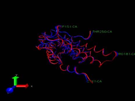
10 The Pressure Profile The Volume Profile For the first 20 ps the pressure is zero. This is to be expected a constant volume simulation was being run in which the pressure was not evaluated. At 20 ps constant pressure conditions were adopted, allowing the volume of the box to change, at which point the pressure dropped sharply becoming negative. The negative pressures correspond to a "force" acting to decrease the box size and the positive pressures to a "force" acting to increase the box size. While the pressure graph seems to show that the pressure fluctuates wildly during the simulation, in actual fact, the mean pressure stabilises as the dynamics proceed which is sufficient to indicate successful equilibration. The volume of the system (in angstroms3) initially decreases as the water box relaxes and reaches an equilibrated density, and thus volume. The smooth transitions in this plot followed by the oscillations about a mean value suggest equilibration has been successful. The Density Profile The system has equilibrated at a density of approximately 1.04 g cm-3 which is reasonable given that the density of pure liquid water at 300 K is approximately 1.00 g cm-3 thus the inference is that the introduction of, in this case the androgen receptor bound to the S-isomer of Vinclozolin and the associated charges has increased the density by around 4 %. The RMSd profile The RMSd of the protein backbone atoms remained low for the first 20 ps, due to the imposed restraints Upon removing the restraints the RMSd increased significantly as the protein relaxed within the solvent After that the RMSd is fairly stable with no wild oscillations Running further equilibration and production MD In the next stage of the simulation a further 1.8 ns of MD were run. Precisely the same conditions were applied as were for the explicit solvent equilibration of the 5 complexes. Namely no restraints on the DNA. Temperature maintained at 300 K using the Langevin thermostat Constant pressure (1 atm) periodic boundaries, SHAKE constraints on the hydrogen atoms and a 2 fs time step. Since 1.8 ns of trajectory were run, output and mdcrd files are written to every 500 fs (250 steps) All of output mdcrd files compressed to save disk space as 1.8 ns of simulation produces very large files Simulation VERY TIME INTENSIVE thus the 1.8 ns broken up into sequential runs i.e. 9 x 200 ps simulations with each successive simulation continuing on from the previous one. Running further equilibration and production MD TIME SPAN (ps) mdrcd OUTPUT FILE Complex1_md2.mdcrd.gz Complex1_md3.mdcrd.gz Complex1_md4.mdcrd.gz Complex1_md5.mdcrd.gz Complex1_md6.mdcrd.gz Complex1_md7.mdcrd.gz Complex1_md8.mdcrd.gz Complex1_md9.mdcrd.gz Complex1_md10.mdcrd.gz 10

11 11