Block Diagram Reduction

Transcription

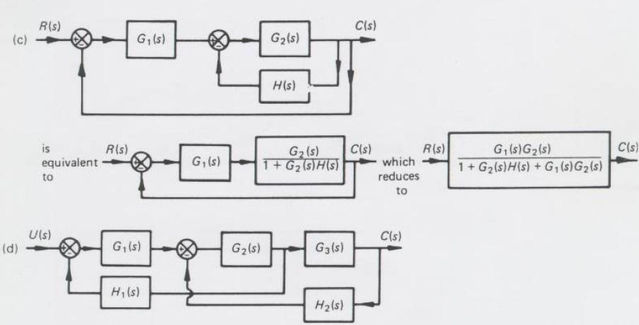
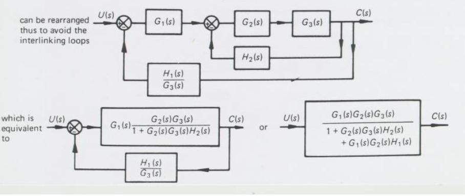
1 Block Diagram Reduction Figure 1: Single block diagram representation Figure 2: Components of Linear Time Invariant Systems (LTIS)

2 Figure 3: Block diagram components Figure 4: Block diagram of a closed-loop system with a feedback element

3 BLOCK DIAGRAM SIMPLIFICATIONS Figure 5: Cascade (Series) Connections Figure 6: Parallel Connections

4 Block Diagram Algebra for Summing Junctions Figure 7: Summing Junctions Block Diagram Algebra for Branch Point Figure 8: Branch Points

5 Block Diagram Reduction Rules Table 1: Block Diagram Reduction Rules Table 2: Basic rules with block diagram transformation

6 Example 1:

7 Example 2: Example 3:

8 Example 4:

9 Example5:

10 ECE 680 Modern Automatic Control Routh s Stability Criterion June 13, ROUTH S STABILITY CRITERION Consider a closed-loop transfer function H(s) = b 0s m + b 1 s m b m 1 s + b m a 0 s n + a 1 s n a n 1 s + a n = B(s) A(s) where the a i s and b i s are real constants and m n. An alternative to factoring the denominator polynomial, Routh s stability criterion, determines the number of closedloop poles in the right-half s plane. (1) Algorithm for applying Routh s stability criterion The algorithm described below, like the stability criterion, requires the order of A(s) to be finite. 1. Factor out any roots at the origin to obtain the polynomial, and multiply by 1 if necessary, to obtain where a 0 0 and a n > 0. a 0 s n + a 1 s n a n 1 s + a n = 0 (2) 2. If the order of the resulting polynomial is at least two and any coefficient a i is zero or negative, the polynomial has at least one root with nonnegative real part. To obtain the precise number of roots with nonnegative real part, proceed as follows. Arrange the coefficients of the polynomial, and values subsequently calculated from them as shown below: s n a 0 a 2 a 4 a 6 s n 1 a 1 a 3 a 5 a 7 s n 2 b 1 b 2 b 3 b 4 s n 3 c 1 c 2 c 3 c 4 s n 4. d 1. d 2. d 3 d 4 (3) s 2 e 1 e 2 s 1 f 1 s 0 g 0 where the coefficients b i are b 1 = a 1a 2 a 0 a 3 a 1 (4) b 2 = a 1a 4 a 0 a 5 a 1 (5) b 3 = a 1a 6 a 0 a 7 a 1 (6).

11 ECE 680 Modern Automatic Control Routh s Stability Criterion June 13, generated until all subsequent coefficients are zero. Similarly, cross multiply the coefficients of the two previous rows to obtain the c i, d i, etc. c 1 = b 1a 3 a 1 b 2 b 1 (7) c 2 = b 1a 5 a 1 b 3 b 1 (8) c 3 = b 1a 7 a 1 b 4 b 1 (9). d 1 = c 1b 2 b 1 c 2 c 1 (10) d 2 = c 1b 3 b 1 c 3 c 1 (11). until the nth row of the array has been completed 1 Missing coefficients are replaced by zeros. The resulting array is called the Routh array. The powers of s are not considered to be part of the array. We can think of them as labels. The column beginning with a 0 is considered to be the first column of the array. The Routh array is seen to be triangular. It can be shown that multiplying a row by a positive number to simplify the calculation of the next row does not affect the outcome of the application of the Routh criterion. 3. Count the number of sign changes in the first column of the array. It can be shown that a necessary and sufficient condition for all roots of (2) to be located in the left-half plane is that all the a i are positive and all of the coefficients in the first column be positive. Example: Generic Quadratic Polynomial. Consider the quadratic polynomial: a 0 s 2 + a 1 s + a 2 = 0 (12) where all the a i are positive. The array of coefficients becomes (13) s 2 a 0 a 2 s 1 a 1 0 s 0 a 2 1 There is one important detail that we have not yet mentioned. If an element of the first column becomes zero, we must alter the procedure. Since this altered procedure is requires some explanation, we postpone discussion of it to a pair of subsections below.

12 ECE 680 Modern Automatic Control Routh s Stability Criterion June 13, where the coefficient a 1 is the result of multiplying a 1 by a 2 and subtracting a 0 (0) then dividing the result by a 2. In the case of a second order polynomial, we see that Routh s stability criterion reduces to the condition that all a i be positive. Example: Generic Cubic Polynomial. Consider the generic cubic polynomial: where all the a i are positive. The Routh array is so the condition that all roots have negative real parts is a 0 s 3 + a 1 s 2 + a 2 s + a 3 = 0 (14) s 3 a 0 a 2 s 2 a 1 a 3 s 1 a 1a 2 a 0 a 3 (15) a 1 s 0 a 3 a 1 a 2 > a 0 a 3. (16) Example: A Quartic Polynomial. Next we consider the fourth-order polynomial: s 4 + 2s 3 + 3s 2 + 4s + 5 = 0. (17) Here we illustrate the fact that multiplying a row by a positive constant does not change the result. One possible Routh array is given at left, and an alternative is given at right, s s s s 1 6 s 0 5 s s Divide this row by two to get s s 1 3 s 0 5 In this example, the sign changes twice in the first column so the polynomial equation A(s) = 0 has two roots with positive real parts. Necessity of all coefficients being positive. In stating the algorithm above, we did not justify the stated conditions. Here we show that all coefficients being positive is necessary for all roots to be located in the left halfplane. It can be shown that any polynomial in s, all of whose coefficients are real, can

13 ECE 680 Modern Automatic Control Routh s Stability Criterion June 13, be factored into a product of a maximal number linear and quadratic factors also having real coefficients. Clearly a linear factor (s + a) has nonnegative real root iff a is positive. For both roots of a quadratic factor (s 2 + bs + c) to have negative real parts both b and c must be positive. (If c is negative, the square root of b 2 4c is real and the quadratic factor can be factored into two linear factors so the number of factors was not maximal.) It is easy to see that if all coefficients of the factors are positive, those of the original polynomial must be as well. To see that the condition is not sufficient, we can refer to several examples above. Example: Determining Acceptable Gain Values So far we have discussed only one possible application of the Routh criterion, namely determining the number of roots with nonnegative real parts. In fact, it can be used to determine limits on design parameters, as shown below. Consider a system whose closed-loop transfer function is The characteristic equation is The Routh array is H(s) = K s(s 2 + s + 1)(s + 2) + K. (18) s 4 + 3s 3 + 3s 2 + 2s 4 + K = 0. (19) s K s s 2 7/3 K s 1 2 9K/7 s 0 K so the s 1 row yields the condition that, for stability, (20) 14/9 > K > 0. (21) Special Case: Zero First-Column Element. If the first term in a row is zero, but the remaining terms are not, the zero is replaced by a small, positive value of ɛ and the calculation continues as described above. Here s an example: s 3 + 2s 2 + s + 2 = 0 (22) has Routh array s s s 1 0 = ɛ s 0 2 (23)

14 ECE 680 Modern Automatic Control Routh s Stability Criterion June 13, where the last element of the first column is equal 2 = (ɛ2 0)/ɛ. In counting changes of sign, the row beginning with ɛ is not counted. If the elements above and below the ɛ in the first column have the same sign, a pair of imaginary roots is indicated. Here, for example, (22) has two roots at s = ±j. On the other hand, if the elements above and below the ɛ have opposite signs, this counts as a sign change. For example, has Routh array with two sign changes in the first column. s 3 3s + 2 = (s 2 1)(s + 2) = 0 (24) s s 2 0 = ɛ 2 s 1 3 2/ɛ s 0 2 Special Case: Zero Row. If all the coefficients in a row are zero, a pair of roots of equal magnitude and opposite sign is indicated. These could be two real roots with equal magnitudes and opposite signs or two conjugate imaginary roots. The zero row is replaced by taking the coefficients of dp (s)/ds, where P (s), called the auxiliary polynomial, is obtained from the values in the row above the zero row. The pair of roots can be found by solving dp (s)/ds = 0. Note that the auxiliary polynomial always has even degree. It can be shown that an auxiliary polynomial of degree 2n has n pairs of roots of equal magnitude and opposite sign. (25) Example: Use of Auxiliary Polynomial Consider the quintic equation A(s) = 0 where A(s) is s 5 + 2s s s (26) The Routh array starts off as s s auxiliary polynomial P (s) s (27) The auxiliary polynomial P (s) is P (s) = 2s s 2 50 (28) which indicates that A(s) = 0 must have two pairs of roots of equal magnitude and opposite sign, which are also roots of the auxiliary polynomial equation P (s) = 0. Taking

15 ECE 680 Modern Automatic Control Routh s Stability Criterion June 13, the derivative of P (s) with respect to s we obtain dp (s) ds = 8s s. (29) so the s 3 row is as shown below and the Routh array is s s s Coefficients of dp (s)/ds s s s 0 50 (30) There is a single change of sign in the first column of the resulting array, indicating that there A(s) = 0 has one root with positive real part. Solving the auxiliary polynomial equation, 2s s 2 50 = 0 (31) yields the remaining roots, namely, from so the original equation can be factored as s 2 = 1, s 2 = 25, (32) s = ±1, s = ±j5. (33) (s + 1)(s 1)(s + j5)(s j5)(s + 2) = 0. (34) Relative stability analysis. Routh s stability criterion provides the answer to the question of absolute stability. This, in many practical cases, is not sufficient. We usually require information about the relative stability of the system. A useful approach for examining relative stability is to shift the s-plane axis and apply Routh s stability criterion. Namely, we substitute s = z σ (σ = constant) into the characteristic equation of the system, write the polynomial in terms of z, and apply Routh s stability criterion to the new polynomial in z. The number of changes of sign in the first column of the array developed for the polynomial in z is equal to the number of roots which are located to the right of the vertical line s = σ. Thus, this test reveals the number of roots which lie to the right of the vertical line s = σ. 2 2 This italicized text and most of the numerical examples are from Section 6-6 of Ogata, Katsuhiko, Modern Control Engineering, Englewood Cliffs, NJ: Prentice-Hall, 1970, pp The rest of the text, including the descriptions of the examples is mine.

16 Similarly, the program for the fourth-order transfer function approximation with T = 0.1 sec is [num,denl = pade(0.1, 4); printsys(num, den, 'st) numlden = sa4-2o0sa O0sA ~ sa sA sA s Notice that the pade approximation depends on the dead time T and the desired order for the approximating transfer function. EXAMPLE PROBLEMS AND SOLUTIONS A-6-1. Sketch the root loci for the system shown in Figure 6-39(a). (The gain K is assumed to be positive.) Observe that for small or large values of K the system is overdamped and for medium values of K it is underdamped. Solution. The procedure for plotting the root loci is as follows: 1. Locate the open-loop poles and zeros on the complex plane. Root loci exist on the negative real axis between 0 and -1 and between -2 and The number of open-loop poles and that of finite zeros are the same.this means that there are no asymptotes in the complex region of the s plane. (2) Figure 6-39 (a) Control system; (b) root-locus plot. Chapter 6 / Root-Locus Analysis

17 3. Determine the breakaway and break-in points.the characteristic equation for the system IS The breakaway and break-in points are determined from dk (2s + l)(s + 2)(s + 3) - s(s + 1)(2> + 5 ) rls [(s + 2)(s + 3)12 as follows: Notice that both points are on root loci. Therefore, they are actual breakaway or break-in points. At point s = , the value of K is Similarly, at s = -2.36h, (Because points = lies between two poles,it is a breakaway point, and because point s = lies between two zeros, it is a break-in point.) 4. Determine a sufficient number of points thd satisfy the angle condition. (It can he found that the root loci involve a circle with center at -1.5 that passes through the breakaway and break-in points.) The root-locus plot for this system is shown in Figure 6-3Y(h). Note that this system is stable for my positive value of K since all the root loci lie in the lefthalf s plane. Small kalues of I*: (0 c K < ) correspond to an overdampcd system. Medium value\ 01' I< ( : K.; 14) correspond to an underdamped system. Finally. large values ol K ( 14 = K ) correspond to an overdamped systern. With a large value of K, the steady state can be I-eachcd in much shorter time than with a \mall value o f I<. The value of K should be adjusted so thal system performance is optimum according to ;I given performance index. Example Problems and Solutions 385

18 A-6-2. Sketch the root loci of the control system shown in Figure 6-40(a). Solution. The open-loop poles are located at s = 0, s = -3 + j4, and s = -3 - j4. A root locus branch exists on the real axis between the origin and -oo.there are three asymptotes for the root 1oci.The angles of asymptotes are &18O0(2k + 1) Angles of asymptotes = = 60, -60, 180" 3 Referring to Equation (6-13), the intersection of the asymptotes and the real axis is obtained as Next we check the breakaway and break-in points. For this system we have Now we set K = -s(s2 + 6s + 25) which yields Figure 6-40 (a) Control system; (b) root-locus plot. Chapter 6 / Root-Locus Analysis

19 Notice that at points s = -2 * ~ the ang!e condition is not satisfied. Hence, they are neither breakaway nor break-in points. In fact, if we calculate the value of K, we obtain (To be an actual breakaway or break-in point, the corresponding value of K must be real and positive.) The angle of departure from the complex pole in the upper half s plane is The points where root-locus branches cross the imaginary axis may be found by substituting s = jw into the characteristic equation and solving the equation for w and K as follows: Noting that the characteristic equation is we have which yields Root-locus branches cross the imaginary axis at w = 5 and w = -S.The value of gain K at the crossing points is 150. Also, the root-locus branch on the real axis touches the imaginary axis at w = 0. Figure 6-40(b) shows a root-locus plot for the svstern. It is noted that if the order of the numerator of G(s)H(s) is lower than that of the denomi- nator by two or more, and if some of the closed-loop poles move on the root locus toward the right as gain K is increased, then other closed-loop poles must move toward the left as gain K is increased.this fact can be seen clearly in this problem. If the gain K is increased from K = 34 to K = 68, the complex-conjugate closed-loop poles are moved from s = to s = -1 + j4: the third pole is moved from s = -2 (which corresponds to K = 34) to s = -4 (which corresponds to K = 68).Thus, the movements of two complex-conjugate closed-loop poles to the right by one unit cause the remaining closed-loop pole (real pole in this case) to move to the left by two units. A-6-3. Consider the system shown in Figure 6-41(a). Sketch the root loci for the system. Observe that for small or large values of K the system is underdamped and for medium values of K it is overdamped. Solution. A root locus exists on the real axis between the origin and -m. The angles of asymptotes of the root-locus branches are obtained as +180 (2k + 1) Angles of asymptotes = = 60, -60, -180" 3 The intersection of the asymptotes and the real axis is located on the real axis at Example Problems and Solutions

20 Figure 6-41 (a) Control system; (bj root-locus plot. (b) The breakaway and break-in points are found from dk/ds = 0. Since the characteristic equation is we have Now we set s3 + 49' + 5s + K = 0 K = -( s3 + 4s2 + 5s). which yields s = -1, s = Since these points are on root loci, they are actual breakaway or break-in points. (At points = -1, the value of K is 2, and at point s = , the value of K is ) The angle of departure from a complex pole in the upper half s plane is obtained from e = go0 or 6 = " The root-locus branch from the complex pole in the upper half s plane breaks into the real axis at s = Next we determine the points where root-locus branches cross the imaginary axis. By substituting s = jw into the characteristic equation, we have or from which we obtain Chapter 6 / Root-Locus Analysis ( j ~ ) ~ + 4(jw)' + 5(jw) + K = 0 (K - 4w2) + jo(5 - w2) = 0 w=rtfl, K=20 or w=o, K=O

21 Root-locus branches cross the imaginary axis at w = fi and w = -fl. The root-locus branch on the real axis touches the jw axis at w = 0. A sketch of the root loci for the system is shown in Figure 641(b). Note that since this system is of third order, there are three closed-loop poles. The nature of the system response to a given input depends on the locations of the closed-loop poles. For 0 < K < 1.852, there are a set of complex-conjugate closed-loop poles and a real closedloop pole. For K < 2, there are three real closed-loop poles. For example, the closedloop poles are located at s = , s = , s = , for K = s = -1, s = -1, s = -2, for K = 2 For 2 < K, there are a set of complex-conjugate closed-loop poles and a real closed-loop pole Thus, small values of K (0 < K < 1.852) correspond to an underdamped system. (Since the real closed-loop pole dominates, only a small ripple may show up in the transient response.) Medium values of K ( K < 2) correspond to an overdamped system. Large values of K (2 < K ) correspond to an underdamped system. With a large value of K, the system responds much faster than with a smaller value of K. Sketch the root loci for the system shown in Figure 6-42(a). Solution. The open-loop poles are located at s = 0, s = -1, s = -2 + j3, and s = -2 - j3. A root locus exists on the real axis between points s = 0 and s = -1. The angles of the asymptotes are found as follows: +180 (2k + 1 ) Angles of asymptotes = = 45", -4j0, 135", 4 (4 Figure 6-42 (a) Control system; (b) root-locus plot. Example Problems and Solutions

22 The intersection of the asymptotes and the real axis is found from The breakaway and break-in points are found from dk/ds = 0. Noting that we have K = -s(s + l)(s2 + 4s + 13) = -(s4 + 5s3 + 17s2 + 13s) from which we get dk = -(4s3 + 15s2 + 34s + 13) = 0 ds Point s = is on a root locus.tl~erefore, it is an actual breakaway point.the gain values K corresponding to points s = f are complex quantities. Since the gain values are not real positive, these points are neither breakaway nor break-in points. The angle of departure from the complex pole in the upper half s plane is Next we shall find the points where root loci may cross the jw axis. Since the characteristic equation is by substituting s = jw into it we obtain from which we obtain w = f , K = or w = 0, K = 0 The root-locus branches that extend to the right-half s plane cross the imaginary axis at w = Also, the root-locus branch on the real axis touches the imaginary axis at w = 0. Figure 6-42(b) shows a sketch of the root loci for the system. Notice that each root-locus branch that extends to the right half s plane crosses its own asymptote. Chapter 6 / Root-Locus Analysis

23 Ad-5. Sketch the root loci for the system shown in Figure 6-43(a). Solution. A root locus exists on the real axis between points s = -1 and s = The asymptotes can be determined as follows: +180 (2k + 1) Angles of asymptotes = = 90, -90" 3-1 The intersection of the asymptotes and the real axis is found from Since the characteristic equation is we have The breakaway and break-in points are found from (3s' + 7.2s)(s + 1) - (s s') - = 0 dk ds (S + Figure 6-43 (a) Control system; (b) root-locus plot. Example Problems and Solutions

24 from which we get Point s = 0 corresponds to the actual breakaway point. But points s = 1.65 f j are neither breakaway nor break-in points, because the corresponding gain values K become complex quantities. To check the points where root-locus branches may cross the imaginary axis, substitute s = jw into the characteristic equation, yielding. ( j ~ + ) 3.6(j~)~ ~ + Kjw + K = 0 A-6-6. Notice that this equation can be satisfied only if w = 0, K = 0. Because of the presence of a double pole at the origin, the root locus is tangent to the jw axis at o = 0. The root-locus branches do not cross the jw axis. Figure 6-43(b) is a sketch of the root loci for this system. Sketch the root loci for the system shown in Figure 6-44(a). Solution. A root locus exists on the real axis between point s = -0.4 and s = The angles of asymptotes can be found as follows: *180 (2k + 1) Angles of asymptotes = = 90, -90" 3-1 Figure 6-44 (a) Control system; (b) root-locus plot. Chapter 6 / Root-Locus Analysis

25 The intersection of the asymptotes and the real axis is obtained from Next we shall find the breakaway points. Since the characteristic equation is we have The breakaway and break-in points are found from from which we get Thus, the breakaway or break-in points are at s = 0 and s = Note that s = -1.2 is a double root. When a double root occurs in dk/ds = 0 at point s = -1.2, d2k/(ds2) = 0 at this point.the value of gain K at point s = -1.2 is This means that with K = 4.32 the characteristic equation has a triple root at points = -1.2.This can be easily verified as follows: Hence, three root-locus branches meet at point s = The angles of departures at point s = -1.2 of the root locus branches that approach the asymptotes are f 180 /3, that is, 60" and -60". (See Problem A-6-7.) Finally, we shall examine if root-locus branches cross the imaginary axis. By substituting s = jw into the characteristic equation, we have This equation can be satisfied only if w = 0, K = 0. At point w = 0, the root locus is tangent to the j o axis because of the presence of a double pole at the origin. There are no points that rootlocus branches cross the imaginary axis. A sketch of the root loci for this system is shown in Figure 6-44(b). Example Problems and Solutions

26 A-6-7. Referring to Problem A-6-6, obtain the equations for the root-locus branches for the system shown in Figure 6-44(a). Show that the root-locus branches cross the real axis at the breakaway point at angles f 60". Solution. The equations for the root-locus branches can be obtained from the angle condition which can be rewritten as By substituting s = u + jw, we obtain /s b - /s = *180 (2k + 1) By rearranging, we have W tan-' (-) - tan-' (:) = tan-' (:) + tan-' (L) *l8o0(2k + 1) u u Taking tangents of both sides of this last equation, and noting that we obtain which can be simplified to which can be further simplified to For u f -1.6, we may write this last equation as Chapter 6 / Root-Locus Analysis

27 which gives the equations for the root-locus as follows: w=o The equation w = 0 represents the real axis. The root locus for 0 5 K 5 co is between points s = -0.4 and s = (The real axis other than this line segment and the origin s = 0 corresponds to the root locus for -w 5 K < 0.) The equations represent the complex branches for 0 5 K 5 m. These two branches lie between a = -1.6 and u = 0. [See Figure 6-44(b).] The slopes of the complex root-locus branches at the breakaway point ( a = -1.2) can be found by evaluating dolda of Equation (6-21) at point a = A-6-8. Since tan-' a = 60, the root-locus branches intersect the real axis with angles +60 Consider the system shown in Figure 6-45(a), which has an unstable feedforward transfer function. Sketch the root-locus plot and locate the closed-loop poles. Show that, although the closedloop poles lie on the negative real axis and the system is not oscillatory, the unit-step response curve will exhibit overshoot. Solution. The root-locus plot for this system is shown in Figure 6-45(b).The closed-loop poles are located at s = -2 and s = -5. The closed-loop transfer function becomes L Closed-loop zero (a) Figure 6-45 :a) Control system; (b) root-locus plot Example Problems and Solutions

28 Figure 6-46 Unit-step response curve for the system shown in Figure 6-45 (a). The unit-step response of this system is The inverse Laplace transform of C(s) gives A-6-9. c(t) = ~-~' e-", fort 2 0 The unit-step response curve is shown in Figure Although the system is not oscillatory, the unit-step response curve exhibits overshoot. (This is due to the presence of a zero at s = -1.) Sketch the root loci of the control system shown in Figure &47(a). Determine the range of gain K for stability. Solution. Open-loop poles are located at s = 1, s = -2 + j d, and s = -2 - j d. A root locus exists on the real axis between points s = 1 and s = -03. The asymptotes of the root-locus branches are found as follows: *180 (2k + 1) Angles of asymptotes = = 60, -60, 180" 3 The intersection of the asymptotes and the real axis is obtained as The breakaway and break-in points can be located from dk/ds = 0. Since we have K = -( r - l)(s2 + 4s + 7) = -(s3 + 3s2 + 3s - 7) which yields Chapter 6 / Root-Locus Analysis (s + I ) = ~ 0

29 (a) Figure 6-47 (a) Control system; (b) root-locus plot. Thus the equation dk/ds = 0 has a double root at 3 = -1. (This means that the characteristic equation has a triple root at s = -1.) The breakaway point is located at s = -1. Three root-locus branches meet at this breakaway point.the angles of departure of the branches at the breakaway point are ilx0 /3, that is. 60" and -60". We shall next determine the points where root-locus branches may cross the imaginary axis. Noting that the characteristic equation is or we substitute s = jw into it and obtain By rewriting this last equation, we have This equation is satisfied when (.r - l)(.s2 + 4s + 7) + K = 0.r + 3, + ~ 3 ~.~- 7 + K = o (jw)' + 3 ( j ~ + ) ~ 3(jw) K - O (K - 7-3w2) +,043 - w2) = 0 = K=7+3w"l6 or w=0, Example Problems and Solutions

30 The root-locus branches cross the imaginary axis at w = hd (where K = 16) and w = 0 (where K = 7). Since the value of gain K at the origin is 7, the range of gain value K for stability is Figure 6-47(b) shows a sketch of the root loci for the system. Notice that all branches consist of parts of straight lines. The fact that the root-locus branches consist of straight lines can be verified as follows: Since the angle condition is we have -1s /s +2 + j fl- /s j d=h180 (2k + 1) By substituting s = a + jw into this last equation, /u j(w + d) + /a j(w - d) = -/a jw f 180 (2k + 1) which can be rewritten as w + a w - v 3 + t ) tan ( ) Taking tangents of both sides of this last equation, we obtain = -tan-'(*) * LW(2k + 1) which can be simplified to 2w(u + 2) w - q2+4ct+4-w2+3 a - 1 or 2w(u + 2)(u - 1) = -w(a2 + 4a W2) w(3a2 + 6u w2) = 0 Further simplification of this last equation yields which defines three lines: 398 Chapter 6 / Root-i.o<cis Analysis

31 Thus the root-locus branches consist of three lines. Note that the root loci for K > 0 consist of portions of the straight lines as shown in Figure 6-47(b). (Note that each straight line starts from an open-loop pole and extends to infinity in the direction of 180, 60, or -60" measured from the real axis.) The remaining portion of each straight line corresponds to K < 0. A Consider the system shown in Figure 6-48(a). Sketch the root loci Solution. The open-loop zeros of the system are located at s = f j. The open-loop poles are located at s = 0 and s = -2. This system involves two poles and two zeros. Hence, there is a possibility that a circular root-locus branch exists. In fact, such a circular root locus exists in this case, as shown in the following. The angle condition is By substituting s = u + jw into this last equation, we obtain Taking tangents of both sides of this equation and noting that Figure 6-48 (a) Control system; (b) root-locus plot. Example Problems and Solutions

32 we obtain which is equivalent to A These two equations are equations for the root 1oci.The first equation corresponds to the root locus on the real axis. (The segment between s = 0 and s = -2 corresponds to the root locus for 0 5 K < m. The remaining parts of the real axis correspond to the root locus for K < 0.) The second equation is an equation for a circle. Thus, there exists a circular root locus with center at u = i, w = 0 and the radius equal to a /2. The root loci are sketched in Figure 6-48(b). [That part of the circular locus to the left of the imaginary zeros corresponds to K > 0. The portion of the circular locus not shown in Figure 6-48(b) corresponds to K < 0.1 Consider the control system shown in Figure Plot the root loci with MATLAB. Solution. MATLAB Program 6-11 generates a root-locus plot as shown in Figure 6-50.The root loci must be symmetric about the real axis. However, Figure 6-50 shows otherwise. MATLAB supplies its own set of gain values that are used to calculate a root-locus plot. It does so by an internal adaptive step-size routine. However, in certain systems, very small changes in the gain cause drastic changes in root locations within a certain range of gains.thus,matlab takes too big a jump in its gain values when calculating the roots, and root locations change by a relatively large amount. When plotting, MATLAB connects these points and causes a strange-looking graph at the location of sensitive gains. Such erroneous root-locus plots typically occur when the loci approach a double pole (or triple or higher pole), since the locus is very sensitive to small gain changes. MATLAB Program num = [O ; den = [I ; rlocus(num,den); v = [ ; axis(v) grid title('root-locus Plot of G(s) = K(s + 0.4)/[sA2(s + 3.6))') Figure 649 Control system. Chapter 6 / Root-Locus Analysis

33 Root-Locus Plot of G(s) = K(s+0.4)/[s2(s+3.6)] Figure (is0 Root-locus lot. Real Axis In the problem considered here, the critical region of gain K is between 4.2 and 4.4.Thus we need to set the step size small enough in this region. We may divide the region for K as tollows: Entering MATLAB Program 6-12 into the computer, we obrain the plot as shown in Figure 6-51, If we change the plot command plot(r,'o') in MATLAB Pr~gram 6-12 to plot(r,'-'1, we obtain Figure Figures 6-51 and 6-52 respectively, show satisfa~tc~ry root-locus plots. MATLAB Program "A, Root-locus plot num = [O 0 I 0.41; den = [I ; K1 = [0:0.2:4.21; K2 = [4.2:0.002:4.4]; K3 = [4.4:0.2:10]; K4 = [I 0:5:200]; K = [KI K2 K3 K4]; r = rlocus(num,den,k); plot(r,'ol) v = [ ; axis(v) grid titie('root-locus Plot of G(s) = K(s + 0.4)/[sA2(s xlabel('rea1 Axis') ylabel('lmag Axis') Example Problems and Solutions

34 5 Root-Locus Plot of G(s) = K(s+O 4)/[s2(s+3.6)] 0 Figure 651 Root-locus plot Real AXIS 0 Root-Locus Plot of G(s) = K(s+0.4)/[s2(s+3.6)] Figure 652 Root-locus plot. A Real Axis Consider the system whose open-loop transfer function G(s)H(s) is given by Using MATLAB, plot root loci and their asymptotes. Solution. We shall plot the root loci and asymptotes on one diagram. Since the open-loop transfer function is given by K G(s)H(s) = - s(s + l)(s + 2) - K s3 + 3s2 + 2s the equation for the asymptotes may be obtained as follows: Noting that K K K lim = lim =- Chapter 6 / Root-Locus Analysis 3+m s3 + 3~~ + 2~ S-'m S~ + 3 ~2 + 3~ + 1 (S + q3

35 the equation for the asymptotes may be given by and for the asymptotes, num = [O O O 11 den = [I numa = [O O O 11 dena = [I In using the following root-locus and plot commands the number of rows of r and that of a must be the same. To ensure this, we include the gain constant K in the commands. For example, MATLAB Program num = [O O O I]; den = [I ; numa = [O I; dena = [I I; K1 = 0:0.1:0.3; K2 = 0.3:0.005:0.5; K3 = 0.5:0.5:10; K4 = 1O:S:I 00; K = [Kl K2 K3 K4]; r = rlocus(num,den,k); a = rlocus(numa,dena,k); y = [r a]; plot(y,'-'1 v = [ ; axis(v) grid title('root-locus Plot of G(s) = K/[s(s + 1 )(s + 2)) and Asymptotes') xlabel('rea1 Axis') ylabeu1lmag Axis') ***** Manually draw open-loop poles in the hard copy ***** Example Problems and Solutions

36 Root-Locus Plot of G(s) = Ki[(.s(s+l)(s+2)] and Asymptotes Figure 6-53 Root-locus plot. Real Axis Including gain K in rlocus command ensures that the r matrix and a matrix have the same number of rows. MATLAB Program 6-13 will generate a plot of root loci and their asymptotes. See Figure Drawing two or more plots in one diagram can also be accomplished by using the hold command. MATLAB Program 6-14 uses the hold command. The resulting root-locus plot is shown in Figure MATLAB Program ~ Root-Locus Plots num = [O I; den = [I ; numa = [O ; dena = ( I; K1 = 0:0.1:0.3; K2 = 0.3:O.OOS:O.S; K3 = O.5:0.5:10; K4 = 10:5:100; K = [Kl K2 K3 K4]; r = rlocus(num,den,k); a = rlocus(numa,dena,k); plot(r,'ol) hold Current plot held plot(a,'-'1 v = [ ; axis(v) grid title('root-locus Plot of G(s) = K/[s(s+l )(s+2)1 and Asymptotes') xlabel('rea1 Axis') ylabel('lmag Axis') Chapter 6 / Root-Locus Analysis

37 Root-Locus Plot of G(s) = Ki[.s(s+l)(s+2)] and Aysmptotes Figure 6-54 Root-locus plot. Real Axis Consider a unity-feedback system with the following feedforward transfer function G(s): K(s + 2)' C(s) = - (s' + 4)(s + 5)' Plot root loci for the system with MATLAB. Solution. A MATLAB program to plot the root loci is given as MATLAB Program The resulting root-locus plot is shown in Figure Notice that this is a special case where no root locus exists on the real axis.this means that for any value of K > 0 the closed-loop poles of the system are two sets of complex-conjugate poles. (No real closed-loop poles exist.) For example, with K = 25, the characteristic equation for the system becomes s4 + 10s' + 54s' + 140s = (sl + 4s + 10)(s2 + 6s + 20) = (S j2.4495)(s j2.44!x)(s ;3.3166)(s j3.3166) MATLAB Program % Root-Locus Plot num = [O ; den = [I ; r = rlocus(nurn,den); plot(r,'ol) hold current plot held plot(r,'-'1 v = [ ; axis(v); axis('squarel) grid title('root-locus Plot of G(s) = (s + 2)"2/[(sA2 + 4)(s + 5)"211) xlabel('rea1 Axis') ylabel('lmag Axis') Example Problems and Solutions

38 Root-Locus Plot of G(s) = (~+2)~/[(~~+4)(s+5)*] Figure 6-55 Root-locus plot. Real Axis Since no closed-loop poles exist in the right-half s plane, the system is stable for all values of K > 0. A Consider a unity-feedback control system with the following feedforward transfer function: Plot a root-locus diagram with MATLAB. Superimpose on the s plane constant 5 lines and constant w, circles. Solution. MATLAB Program 6-16 produces the desired plot as shown in Figure MATLAB Program num = [ ; den = [I ; K = 0:0.2:200; rlocus(num,den,k) v = [ ; axis(v1; axis('squarel) sgrid title('root-locus Plot with Constant \zeta Lines and Constant \omega-n Circles') gtext('\zeta = 0.9') gtext('0.7') gtext('0.5') gtext('0.3') gtext('\omega-n = 10') gtext('8') gtext('6') gtext('4') gtext('2') Chapter 6 / Root-Locus Analysis

39 Root-Locus Plot with Constant ( Lines and Constant on Circles Figure 6-56 Root-locus plot with constant 6 lilies and constant w,, c:ircles. Real Axis A Consider a unity-feedback control system with the following feedforward transfer function: Plot root loci for the system with MATLAB. Show that the system is stable for all values of K > 0. Solution. MATLAB Program 6-17 gives a plot of root loci as shown in Figure Since the root loci are entirely in the left-half s plane, the system is stable for all K > 0. MATLAB Program num = [O ; den = [I ; K = 0:0.4:1000; rlocus(num,den,k) v = [ ; axis(v); axis('square') grid title('root-locus Plot of G(s) = K(sA2 + 25)s/(sA sA )') A A simplified form of the open-loop transfer function of an airplane with an autopilot in the longitudinal mode is Such a system involving an open-loop pole in the right-half s plane may be conditionally stable. Sketch the root loci when a = b = 1, (' = 0.5, and w,, = 4. Find the range of gain K for stability. Example Problems and Solutions 407

40 Root-Locus Plot of G(s) = ~ ( + 25)s/(s4 s ~ + 404s ) Figure 6-57 Root-locus plot. Real Axis Solution. The open-loop transfer function for the system is To sketch the root loci, we follow this procedure: 1. Locate the open-loop poles and zero in the complex plane. Root loci exist on the real axis between 1 and 0 and between -1 and -m. 2. Determine the asymptotes of the root loci.there are three asymptotes whose angles can be determined as 180 (2k + 1) Angles of asymptotes = = 60, -60, 180" 4-1 Referring to Equation (6-13), the abscissa of the intersection of the asymptotes and the real axis is 3. Determine the breakaway and break-in points. Since the characteristic equation is we obtain By differentiating K with respect to s, we get Chapter 6 / Root-Locus Analysis

41 The numerator can be factored as follows: 3s4 + 10s3 + 21s2 + 24s - 16 Points s = 0.45 and s = are on root loci on the real axis. Hence, these points are actual breakaway and break-in points, respectively. Points s = f do not satisfy the angle condition. Hence, they are neither breakawav nor break-in points. 4. Using Routh's stability criterion, determine the value of K at which the root loci cross the imaginary axis. Since the characteristic equation is the Routh array becomes The values of K that make the s' term in the first column equal zero are K = 35.7 and K = The crossing points on the imaginary axis can be found by solving the auxiliary equation obtained from the s2 row, that is, by solving the following equation for s: The results are s = kj2.56, for K = 35.7 s = ij1.56, for K = 23.3 The crossing points on the imaginary axis are thus s = ~tj2.56 and s = ij Find the angles of departure of the root loci from the complex poles. For the open-loop pole at s = -2 + j 2d, the angle of departure 8 is or H = -54.5" (The angle of departure from the open-loop pole at s = -2-12fl is 54S0.) 6. Choose a test point in the broad neighborhood of the jw axis and the origin, and apply the angle condition. If the test point does not satisfy the angle condition, select another test point until it does. Continue the same process and locate a sufficient number of points that satisfy the angle condition. Example Problems and Solutions 409

42 Figure 6-58 Root-locus plot. Figure 6-58 shows the root loci for this system. From step 4, the system is stable for 23.3 < K < Otherwise, it is unstable.thus, the system is conditionally stable. Consider the system shown in Figure 6-59, where the dead time T is 1 sec. Suppose that we approximate the dead time by the second-order pade approximation. The expression for this approximation can be obtained with MATLAB as follows: [num,den] = pade(1, 2); printsys(num, den) numlden = s"2-6s + 12 Hence Using this approximation, determine the critical value of K (where K > 0) for stability. Solution. Since the characteristic equation for the system is s Ke-" = 0 Chapter 6 / Root-Locus Analysis

43 Figure 6-59 A control system with dead time. by substituting Equation (6-22) into this characteristic equation, we obtain Applying the Routh stability criterion, we get the Routh table as follows: Hence, for stability we require which can be written as or -6K2-36K > 0 (K )(K ) < 0 K < Since K must be positive, the range of K for stability is 0 < K < Notice that according to the present analysis, the upper limit of K for stability is This value is greater than the exact upper limit of K. (Earlier, we obtained the exact upper limit of K to be 2, as shown in Figure 6-38.) This is because we approximated e-" by the second-order pade approximation. A higher-order pade approximation will improve the accuracy. However, the computations involved increase considerably. A Consider the system shown in Figure 6-60.The plant involves the dead time of T sec. Design a suitable controller G,(s) for the system. Solution. We shall present the Smith predictor approach to design a controller. The first step to design the controller G,(s) is to design a suitable controller G, (s) when the system has no dead time. Otto J. M. Smith designed an innovative controller scheme, now called the "Smith predictor," Example Problems and Solutions 41 1

44

45 Then the closed-loop transfer function C(s)/R(s) can be given by Hence, the block diagram of Figure 6-61(a) can be modified to that of Figure 6-61(b).The closedloop response of the system with dead time e-tjis the same as the response of the system without dead time c-~', except that the response is delayed by T sec. Typical step-response curves of the system without dead time controlled by the controller &,(s) and of the system with dead time controlled by the Smith predictor type controller are shown in Figure It is noted that implementing the Smith predictor in digital form is not difficult, because dead time can be handled easily in digital control. However, implementing the Smith predictor in an analog form creates some difficulty. Step Response Sm~th predictor type controller Figure 6-62 Step-response curves Time (sec) PROBLEMS B-6-1. Plot the root loci for the closed-loop control system B-6-3. Plot the root loci for the closed-loop control system with with B-6-2. Plot the root loci for the closed-loop control system with B-6-4. Plot the root loci for the system with.. Problems 413

46 B-6-5. Plot the root loci for a system with B Consider the system whose open-loop transfer function G(s)H(s) is given by Determine the exact points where the root loci cross the jw axis Show that the root loci for a control system with Plot a root-locus diagram with MATLAB. B Consider the system whose open-loop transfer function is given by are arcs of the circle centered at the origin with radius equal to m Plot the root loci for a closed-loop control system with Show that the equation for the asymptotes is given by B-6-8. with Plot the root loci for a closed-loop control system Using MATLAB, plot the root loci and asymptotes for the svstem. B Consider the unity-feedback system whose feedforward transfer function is B-6-9. with Plot the root loci for a closed-loop control system Locate the closed-loop poles on the root loci such that the dominant closed-loop poles have a damping ratio equal to 0.5. Determine the corresponding value of gain K. B Plot the root loci for the system shown in Figure Determine the range of gain K for stability. The constant-gain locus for the system for a given value of K is defined by the following equation: Show that the constant-gain loci for 0 5 K 5 co may be given by Figure 6-63 Control system. Sketch the constant-gain loci for K = 1,2,5,10, and 20 on the s plane. B Consider the system shown in Figure Plot the root loci with MATLAB. Locate the closed-loop poles when the gain K is set equal to 2. R Consider a unity-feedback control system with the following feedforward transfer function: Plot the root loci for the system. If the value of gain K is set equal to 2, where are the closed-loop poles located? 414 Chapter 6 / Root-Locus Analysis Figure 6-64 Control system. u

47 B Plot root-locus diagrams for the nonminimum- B Consider the closed-loop system with transport lag phase systems shown in Figures 6-65(a) and (b), respectively. shown in Figure Determine the stability range for gain K. Figure 6-66 Control system. Figure 4-65 (a) and (b) Nonminimum-phase systems. Problems