Control Systems Engineering ( Chapter 6. Stability ) Prof. Kwang-Chun Ho Tel: Fax:
|
|
|
- Cleopatra Booth
- 5 years ago
- Views:
Transcription
1 Control Systems Engineering ( Chapter 6. Stability ) Prof. Kwang-Chun Ho kwangho@hansung.ac.kr Tel: Fax:
2 Introduction In this lesson, you will learn the following : How to determine the stability of a system represented as a transfer function How to determine the stability of a system represented in state-space How to determine system parameters to yield stability 2
3 Introduction What is stability? Most important system specification We cannot use a control system if the system is unstable Stability is subjective There are many definitions for stability, depending on the kind of system or the point of view We limit ourselves to linear time invariant (LTI) systems The total response of a system is the sum of the forced and natural response, ct c t c t forced natural 3
4 Introduction Using these concepts, we present the following definitions of stability, instability and marginal stability A linear time invariant system is stable if the natural response approaches to zero as time approaches to infinity A linear time invariant system is unstable if the natural response grows without bound as time approaches to infinity A linear time invariant system is marginally stable if the natural response neither decays nor grows but remains constant or oscillates as time approaches to infinity An alternative and best-known definition of stability is as follows : A system is stable if every bounded input yields a bounded output We call this statement the bounded-input, bounded-output (BIBO) definition of stability 4
5 Introduction How do we determine if a system is stable? If the closed loop system poles are in the left-half of the s-plane and hence have a negative real part, the system is stable Unstable systems have closed loop system transfer functions with at least one pole at the right half plane and/or poles of multiplicity greater than one on the imaginary axis Similarly, marginally stable systems have closed loop transfer function with only imaginary axis poles of multiplicity 1 and poles in the left half plane As an example, the unit step responses of a stable and an unstable system are shown in figure (a) and (b) 5
6 Introduction Marginally stable 6
7 In this section, we will learn a method that yields stability information without the need to solve for closed loop system poles The method is called the Routh-Hurwitz criterion for stability (Routh, 1905) The method requires two steps : Generate a data table called a Routh table Interpret the Routh table to tell how many closed loop system poles are in the left half plane, the right half plane, and on the imaginary axis Generating a Basic Routh Table: Look at the equivalent closed-loop transfer function shown in figure 7
8 Since we are interested in the system poles, we focus our attention on the denominator We first create the Routh table shown in Table Begin by labelling the rows with powers of s from the highest power of the denominator of the closed loop transfer function to s 0 8
9 Next, start with the coefficient of the highest power of s in the denominator and list, horizontally in the first row, every other coefficient In the second row, list horizontally, starting with the highest power of s, every coefficient that was skipped in the first row The remaining entries are filled in as follows: Each entry is a negative determinant of entries in the previous two rows divided by the entry in the first column directly above the calculated row The left-hand column of the determinant is always the first column of the previous two rows, and the right-hand column is the elements of the column above and to the right The table is complete when all of the rows are completed down to s 0 Table 6.2 is the completed Routh table 9
10 Example: Make the Routh table for the system shown in the figure 10
11 Solution: The first step is to find the equivalent closed loop system because we want to test the denominator of this function, not the given forward transfer function, for pole location Using the feedback formula, we obtain the equivalent system of figure(b) The Routh-Hurwitz criterion will be applied to this denominator 11
12 First, label the rows with powers of s from s 3 down to s 0 in a vertical column Next, form the first row of the table, using the coefficients of the denominator Start with the coefficient of the highest power and skip every other power of s Now form the second row with the coefficients of the denominator skipped in the previous step Subsequent rows are formed with determinants as shown in table For convenience, any row of the Routh table can be multiplied by a positive constant without changing the values of rows below For example, in the second row of table, the row was multiplied by 1/10 Interpreting the Basic Routh Table : Now that we know how to generate the Routh table, let us see how to interpret it 12
13 Simply stated, the Routh-Hurwitz criterion declares that the number of roots of the polynomial that are in the right half plane is equal to the number of sign changes in the first column If the closed loop transfer function has all poles in the left half of the s-plane, the system is stable Thus, a system is stable if there are no sign changes in the first column of the Routh table For example, the following table has two sign changes in the first column The first sign changes occurs from 1 in the s 2 row to -72 in the s 1 row The second occurs from -72 in the s 1 row to 103 in the s 0 row Thus, the system is unstable since two poles exist in the right half plane 13
14 Example: Make a Routh table and tell how many roots of the following polynomial are in the right half-plane and in the left half-plane Solution: P s 3s 9s 6s 4s 7s 8s 2s 6 14
15 : Special Cases Two special cases can occur: The Routh table sometimes will have a zero only in the first column of a row The Routh table sometimes will have an entire row that consists of zeros Example: Determine the stability of the closed loop transfer function Solution: Begin by assembling the Routh table down to the row where a zero appears only in the first column (the s 3 row) Next replace the zero by a very small number,, and complete the table 10 T ( s) s 2s 3s 6s 5s 3 15
16 (a) (b) To begin the interpretation, we must firs assume a sign, positive or negative, for the quantity, table(b) shows the first column of table(a) along with the resulting signs for choices of positive and negative If is chosen negative table(b) will show a sign change from the s 3 row to the s 2 row, and there will be another sign change from the s 2 row to the s 1 row 16
17 Example: Hence, the system is unstable and has two poles in the right half plane Alternatively, we could choose negative Table(b) would then show a sign change from the s 4 row to the s 3 row Another sign change would occur from the s 3 row to the s 2 row One result would be exactly the same as that for a positive choice for Thus, the system is unstable, with two poles in the right half plane Tell how many roots of the following polynomial are in the right half-plane, in the left half-plane, and on the -axis: Solution: j Q s s 2s 2s 4s 11s 10 17

18 Example: Entire Row is Zero Tell how many roots of the following polynomial are in the right half-plane, in the left half-plane, and on the j -axis: Q s s s 3s 2s 2 Solution:
 5 4 3 2 s 7s 6s 42s (Have 2 poles on the j -axis and 2 poles in the left-half plane) 8s 56")
19 Example: When a Routh table has entire row of zeros, the poles could be in the right half plane, or the left half plane or on the j -axis Determine the number of right-half-plane poles in the closed transfer function 10 T ( s) s 7s 6s 42s (Have 2 poles on the j -axis and 2 poles in the left-half plane) 8s 56 19
20 Solution: Start by the forming the Routh table for the denominator At the second row, we multiply through by 1/7 for convenience We stop at the third row, since the entire row consists of the zeros, and use the following procedure First, we return to row immediately above the row of zeros and form an auxiliary polynomial, using the entries in that row as coefficients The polynomial will start with the power of s in the label column and continue by skipping every other power of s 20
21 Example: Thus, the even polynomial formed for this example is Next, we differentiate the polynomial with respect to s, and obtain Finally, we use the coefficients of the last equation to replace the row of zeros Again, for convenience, the third row is multiplied by 1/4 after replacing zeros There are no sign changes, so there are no poles on the right half plane. The system is marginally stable! For the transfer function Ps s s 4 2 () 6 8 dp() s s s ds
22 tell how many poles are the right half plane, or the left half plane or on the -axis Solution j At the s 3 row, we obtain a row of zeros 22
23 Moving back one row to s 4, we extract the even polynomial, P(s), as Taking the derivative for x to obtain the coefficients that replace the row of zeros in the s 3 row, we find Finally, continue the table to the s 0 row, using standard procedure How do we now interpret the Routh table? No sign changes exist from the s 4 row down to the s 0 row Thus, there are no right-half plane poles and the P(s) has all four of its poles on the j -axis The remaining roots of polynomial evaluated from the s 8 row down to the s 4 row have two sign changes and two no sign changes Thus, it has two poles in the right-half plane and the left-half plane, respectively 23
24 Unstable!! Example: Stability Design via Routh-Hurwitz Find the range of the gain K, for the system shown below that will cause the system to be stable, unstable and marginally stable. Assume K > 0 24
25 Solution: First find the closed-loop transfer function as K Gs () ss ( 7)( s 11) K T() s Gs ( ) K 1 s 18s 77s K ss ( 7)( s 11) Next form the Routh table 25
26 Since K assumed positive, we see that all elements in the first column are always positive except the s 1 row This entry can be positive, zero, or negative, depending upon the value of K If K <1386, all terms in the first column will be positive, and since there are no sign changes, the system will have three poles at the left-half plane and be stable(0<k<1386) If K =1386, we have an entire row of zeros, which could signify poles Returning the s 2 row and replacing K with 1386, we form the even polynomial Ps 2 ( ) 18s 1386 Differentiating with respect to s, we obtain dp() s ds 36s 0 j 26
27 Replacing the row of zeros with the coefficients of the last equation, we obtain the following Routh table Since there are no sign changes from the even polynomial (s 2 row) down to the bottom of the table, the even polynomial has its two roots on the j -axis of the unit multiplicity Since there are no sign changes above the even polynomial, the remaining root is in the left-half plane Therefore, the system is marginally stable! 27
28 Stability in State Space Up to this point, we have examined stability from the s- plane viewpoint Now we look at stability from the perspective of state space We know that the values of the system poles are equal to the eigenvalues of the system matrix We stated that the eigenvalues of matrix A were solutions of the equation det(i-a) s, which also yielded the poles of the transfer function (discussed in chapter 3!) 28
29 Example: For the system given below, find out how many poles are in the left half plane, in the right half plane, and on the j -axis x x 0 u, y x Solution: (I-A) s First form : s s 3 1 ( si A) 0 s s s s 2 29
30 det(i-a) s Now find the : 3 2 det( si A) s 6s 7s 52 Using this polynomial, form the Routh table Since there is one sign change in the first column, the system has one right half plane pole and two left half plane poles It is therefore unstable 30
31 Homework Assignment #6 (Use Routh table) 31
32 Homework Assignment #6 32
33 Homework Assignment #6 33
34 Homework Assignment #6 34
Remember that : Definition :
 Stability This lecture we will concentrate on How to determine the stability of a system represented as a transfer function How to determine the stability of a system represented in state-space How to
Software Engineering/Mechatronics 3DX4. Slides 6: Stability
 Software Engineering/Mechatronics 3DX4 Slides 6: Stability Dr. Ryan Leduc Department of Computing and Software McMaster University Material based on lecture notes by P. Taylor and M. Lawford, and Control
Outline. Control systems. Lecture-4 Stability. V. Sankaranarayanan. V. Sankaranarayanan Control system
 Outline Control systems Lecture-4 Stability V. Sankaranarayanan Outline Outline 1 Outline Outline 1 2 Concept of Stability Zero State Response: The zero-state response is due to the input only; all the
Control Systems Engineering ( Chapter 8. Root Locus Techniques ) Prof. Kwang-Chun Ho Tel: Fax:
 Prof. Kwang-Chun Ho Tel: Fax:") Control Systems Engineering ( Chapter 8. Root Locus Techniques ) Prof. Kwang-Chun Ho kwangho@hansung.ac.kr Tel: 02-760-4253 Fax:02-760-4435 Introduction In this lesson, you will learn the following : The
Control Systems Engineering ( Chapter 8. Root Locus Techniques ) Prof. Kwang-Chun Ho kwangho@hansung.ac.kr Tel: 02-760-4253 Fax:02-760-4435 Introduction In this lesson, you will learn the following : The
Lecture 4 Classical Control Overview II. Dr. Radhakant Padhi Asst. Professor Dept. of Aerospace Engineering Indian Institute of Science - Bangalore
 Lecture 4 Classical Control Overview II Dr. Radhakant Padhi Asst. Professor Dept. of Aerospace Engineering Indian Institute of Science - Bangalore Stability Analysis through Transfer Function Dr. Radhakant
I Stable, marginally stable, & unstable linear systems. I Relationship between pole locations and stability. I Routh-Hurwitz criterion
 EE C128 / ME C134 Feedback Control Systems Lecture Chapter 6 Stability Lecture abstract Alexandre Bayen Department of Electrical Engineering & Computer Science University of California Berkeley Topics
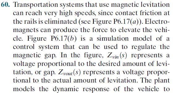
ECE317 : Feedback and Control
 ECE317 : Feedback and Control Lecture : Routh-Hurwitz stability criterion Examples Dr. Richard Tymerski Dept. of Electrical and Computer Engineering Portland State University 1 Course roadmap Modeling
Some special cases
 Lecture Notes on Control Systems/D. Ghose/2012 87 11.3.1 Some special cases Routh table is easy to form in most cases, but there could be some cases when we need to do some extra work. Case 1: The first
EEE 184: Introduction to feedback systems
 EEE 84: Introduction to feedback systems Summary 6 8 8 x 7 7 6 Level() 6 5 4 4 5 5 time(s) 4 6 8 Time (seconds) Fig.. Illustration of BIBO stability: stable system (the input is a unit step) Fig.. step)
ECE317 : Feedback and Control
 ECE317 : Feedback and Control Lecture : Stability Routh-Hurwitz stability criterion Dr. Richard Tymerski Dept. of Electrical and Computer Engineering Portland State University 1 Course roadmap Modeling
ECEN 605 LINEAR SYSTEMS. Lecture 20 Characteristics of Feedback Control Systems II Feedback and Stability 1/27
 1/27 ECEN 605 LINEAR SYSTEMS Lecture 20 Characteristics of Feedback Control Systems II Feedback and Stability Feedback System Consider the feedback system u + G ol (s) y Figure 1: A unity feedback system
HANDOUT E.22 - EXAMPLES ON STABILITY ANALYSIS
 Example 1 HANDOUT E. - EXAMPLES ON STABILITY ANALYSIS Determine the stability of the system whose characteristics equation given by 6 3 = s + s + 3s + s + s + s +. The above polynomial satisfies the necessary
EE Control Systems LECTURE 9
 Updated: Sunday, February, 999 EE - Control Systems LECTURE 9 Copyright FL Lewis 998 All rights reserved STABILITY OF LINEAR SYSTEMS We discuss the stability of input/output systems and of state-space
Control Systems. Internal Stability - LTI systems. L. Lanari
 Control Systems Internal Stability - LTI systems L. Lanari outline LTI systems: definitions conditions South stability criterion equilibrium points Nonlinear systems: equilibrium points examples stable
(b) A unity feedback system is characterized by the transfer function. Design a suitable compensator to meet the following specifications:
 A unity feedback system is characterized by the transfer function. Design a suitable compensator to meet the following specifications:") 1. (a) The open loop transfer function of a unity feedback control system is given by G(S) = K/S(1+0.1S)(1+S) (i) Determine the value of K so that the resonance peak M r of the system is equal to 1.4.
1. (a) The open loop transfer function of a unity feedback control system is given by G(S) = K/S(1+0.1S)(1+S) (i) Determine the value of K so that the resonance peak M r of the system is equal to 1.4.
7.4 STEP BY STEP PROCEDURE TO DRAW THE ROOT LOCUS DIAGRAM
 ROOT LOCUS TECHNIQUE. Values of on the root loci The value of at any point s on the root loci is determined from the following equation G( s) H( s) Product of lengths of vectors from poles of G( s)h( s)
S I X SOLUTIONS TO CASE STUDIES CHALLENGES. Antenna Control: Stability Design via Gain K s s s+76.39K. T(s) =
 =") S I X Stability SOLUTIONS TO CASE STUDIES CHALLENGES Antenna Control: Stability Design via Gain From the antenna control challenge of Chapter 5, Make a Routh table: 76.39K s 3 +151.32s 2 +198s+76.39K s
S I X Stability SOLUTIONS TO CASE STUDIES CHALLENGES Antenna Control: Stability Design via Gain From the antenna control challenge of Chapter 5, Make a Routh table: 76.39K s 3 +151.32s 2 +198s+76.39K s
ECE 345 / ME 380 Introduction to Control Systems Lecture Notes 8
 Learning Objectives ECE 345 / ME 380 Introduction to Control Systems Lecture Notes 8 Dr. Oishi oishi@unm.edu November 2, 203 State the phase and gain properties of a root locus Sketch a root locus, by
Lecture 10: Proportional, Integral and Derivative Actions
 MCE441: Intr. Linear Control Systems Lecture 10: Proportional, Integral and Derivative Actions Stability Concepts BIBO Stability and The Routh-Hurwitz Criterion Dorf, Sections 6.1, 6.2, 7.6 Cleveland State
EE 380. Linear Control Systems. Lecture 10
 EE 380 Linear Control Systems Lecture 10 Professor Jeffrey Schiano Department of Electrical Engineering Lecture 10. 1 Lecture 10 Topics Stability Definitions Methods for Determining Stability Lecture 10.
STABILITY ANALYSIS. Asystemmaybe stable, neutrallyormarginallystable, or unstable. This can be illustrated using cones: Stable Neutral Unstable
 ECE4510/5510: Feedback Control Systems. 5 1 STABILITY ANALYSIS 5.1: Bounded-input bounded-output (BIBO) stability Asystemmaybe stable, neutrallyormarginallystable, or unstable. This can be illustrated
Analysis of Stability &
 INC 34 Feedback Control Sytem Analyi of Stability & Steady-State Error S Wonga arawan.won@kmutt.ac.th Summary from previou cla Firt-order & econd order ytem repone τ ωn ζω ω n n.8.6.4. ζ ζ. ζ.5 ζ ζ.5 ct.8.6.4...4.6.8..4.6.8
I What is root locus. I System analysis via root locus. I How to plot root locus. Root locus (RL) I Uses the poles and zeros of the OL TF
 I Uses the poles and zeros of the OL TF") EE C28 / ME C34 Feedback Control Systems Lecture Chapter 8 Root Locus Techniques Lecture abstract Alexandre Bayen Department of Electrical Engineering & Computer Science University of California Berkeley
EE C28 / ME C34 Feedback Control Systems Lecture Chapter 8 Root Locus Techniques Lecture abstract Alexandre Bayen Department of Electrical Engineering & Computer Science University of California Berkeley
Root Locus Methods. The root locus procedure
 Root Locus Methods Design of a position control system using the root locus method Design of a phase lag compensator using the root locus method The root locus procedure To determine the value of the gain
ECE 388 Automatic Control
 Controllability and State Feedback Control Associate Prof. Dr. of Mechatronics Engineeering Çankaya University Compulsory Course in Electronic and Communication Engineering Credits (2/2/3) Course Webpage:
Software Engineering 3DX3. Slides 8: Root Locus Techniques
 Software Engineering 3DX3 Slides 8: Root Locus Techniques Dr. Ryan Leduc Department of Computing and Software McMaster University Material based on Control Systems Engineering by N. Nise. c 2006, 2007
Stability Analysis Techniques
 Stability Analysis Techniques In this section the stability analysis techniques for the Linear Time-Invarient (LTI) discrete system are emphasized. In general the stability techniques applicable to LTI
Test 2 SOLUTIONS. ENGI 5821: Control Systems I. March 15, 2010
 Test 2 SOLUTIONS ENGI 5821: Control Systems I March 15, 2010 Total marks: 20 Name: Student #: Answer each question in the space provided or on the back of a page with an indication of where to find the
Control Systems I. Lecture 7: Feedback and the Root Locus method. Readings: Jacopo Tani. Institute for Dynamic Systems and Control D-MAVT ETH Zürich
 Control Systems I Lecture 7: Feedback and the Root Locus method Readings: Jacopo Tani Institute for Dynamic Systems and Control D-MAVT ETH Zürich November 2, 2018 J. Tani, E. Frazzoli (ETH) Lecture 7:
Root locus 5. tw4 = 450. Root Locus S5-1 S O L U T I O N S
 Root Locus S5-1 S O L U T I O N S Root locus 5 Note: All references to Figures and Equations whose numbers are not preceded by an "S" refer to the textbook. (a) Rule 2 is all that is required to find the
Vulnerability Analysis of Feedback Systems
 Vulnerability Analysis of Feedback Systems Nathan Woodbury Advisor: Dr. Sean Warnick Honors Thesis Defense 11/14/2013 Acknowledgements Advisor Dr. Sean Warnick Honors Committee Dr. Scott Steffensen Dr.
Chemical Process Dynamics and Control. Aisha Osman Mohamed Ahmed Department of Chemical Engineering Faculty of Engineering, Red Sea University
 Chemical Process Dynamics and Control Aisha Osman Mohamed Ahmed Department of Chemical Engineering Faculty of Engineering, Red Sea University 1 Chapter 4 System Stability 2 Chapter Objectives End of this
Control Systems. Internal Stability - LTI systems. L. Lanari
 Control Systems Internal Stability - LTI systems L. Lanari definitions (AS) - A system S is said to be asymptotically stable if its state zeroinput response converges to the origin for any initial condition
Poles, Zeros and System Response
 Time Response After the engineer obtains a mathematical representation of a subsystem, the subsystem is analyzed for its transient and steady state responses to see if these characteristics yield the desired
Controls Problems for Qualifying Exam - Spring 2014
 Controls Problems for Qualifying Exam - Spring 2014 Problem 1 Consider the system block diagram given in Figure 1. Find the overall transfer function T(s) = C(s)/R(s). Note that this transfer function
STABILITY OF CLOSED-LOOP CONTOL SYSTEMS
 CHBE320 LECTURE X STABILITY OF CLOSED-LOOP CONTOL SYSTEMS Professor Dae Ryook Yang Spring 2018 Dept. of Chemical and Biological Engineering 10-1 Road Map of the Lecture X Stability of closed-loop control
Routh-Hurwitz Lecture Routh-Hurwitz Stability test
 ECE 35 Routh-Hurwitz Leture Routh-Hurwitz Staility test AStolp /3/6, //9, /6/ Denominator of transfer funtion or signal: s n s n s n 3 s n 3 a s a Usually of the Closed-loop transfer funtion denominator
Control Systems I. Lecture 9: The Nyquist condition
 Control Systems I Lecture 9: The Nyquist condition Readings: Åstrom and Murray, Chapter 9.1 4 www.cds.caltech.edu/~murray/amwiki/index.php/first_edition Jacopo Tani Institute for Dynamic Systems and Control
Stability of Feedback Control Systems: Absolute and Relative
 Stability of Feedback Control Systems: Absolute and Relative Dr. Kevin Craig Greenheck Chair in Engineering Design & Professor of Mechanical Engineering Marquette University Stability: Absolute and Relative
Chapter 7 : Root Locus Technique
 Chapter 7 : Root Locus Technique By Electrical Engineering Department College of Engineering King Saud University 1431-143 7.1. Introduction 7.. Basics on the Root Loci 7.3. Characteristics of the Loci
Laplace Transform Analysis of Signals and Systems
 Laplace Transform Analysis of Signals and Systems Transfer Functions Transfer functions of CT systems can be found from analysis of Differential Equations Block Diagrams Circuit Diagrams 5/10/04 M. J.
Stability Criterion Routh Hurwitz
 EES404 Fundamental of Control Sytem Stability Criterion Routh Hurwitz DR. Ir. Wahidin Wahab M.Sc. Ir. Arie Subiantoro M.Sc. Stability A ytem i table if for a finite input the output i imilarly finite A
r + - FINAL June 12, 2012 MAE 143B Linear Control Prof. M. Krstic
 MAE 43B Linear Control Prof. M. Krstic FINAL June, One sheet of hand-written notes (two pages). Present your reasoning and calculations clearly. Inconsistent etchings will not be graded. Write answers
SECTION 5: ROOT LOCUS ANALYSIS
 SECTION 5: ROOT LOCUS ANALYSIS MAE 4421 Control of Aerospace & Mechanical Systems 2 Introduction Introduction 3 Consider a general feedback system: Closed loop transfer function is 1 is the forward path
ECE504: Lecture 9. D. Richard Brown III. Worcester Polytechnic Institute. 04-Nov-2008
 ECE504: Lecture 9 D. Richard Brown III Worcester Polytechnic Institute 04-Nov-2008 Worcester Polytechnic Institute D. Richard Brown III 04-Nov-2008 1 / 38 Lecture 9 Major Topics ECE504: Lecture 9 We are
3 Stabilization of MIMO Feedback Systems
 3 Stabilization of MIMO Feedback Systems 3.1 Notation The sets R and S are as before. We will use the notation M (R) to denote the set of matrices with elements in R. The dimensions are not explicitly
Identification Methods for Structural Systems. Prof. Dr. Eleni Chatzi System Stability - 26 March, 2014
 Prof. Dr. Eleni Chatzi System Stability - 26 March, 24 Fundamentals Overview System Stability Assume given a dynamic system with input u(t) and output x(t). The stability property of a dynamic system can
Alireza Mousavi Brunel University
 Alireza Mousavi Brunel University 1 » Control Process» Control Systems Design & Analysis 2 Open-Loop Control: Is normally a simple switch on and switch off process, for example a light in a room is switched
Lecture 1 Root Locus
 Root Locus ELEC304-Alper Erdogan 1 1 Lecture 1 Root Locus What is Root-Locus? : A graphical representation of closed loop poles as a system parameter varied. Based on Root-Locus graph we can choose the
Module 3F2: Systems and Control EXAMPLES PAPER 2 ROOT-LOCUS. Solutions
 Cambridge University Engineering Dept. Third Year Module 3F: Systems and Control EXAMPLES PAPER ROOT-LOCUS Solutions. (a) For the system L(s) = (s + a)(s + b) (a, b both real) show that the root-locus
KINGS COLLEGE OF ENGINEERING DEPARTMENT OF ELECTRONICS AND COMMUNICATION ENGINEERING
 KINGS COLLEGE OF ENGINEERING DEPARTMENT OF ELECTRONICS AND COMMUNICATION ENGINEERING QUESTION BANK SUB.NAME : CONTROL SYSTEMS BRANCH : ECE YEAR : II SEMESTER: IV 1. What is control system? 2. Define open
Nyquist Criterion For Stability of Closed Loop System
 Nyquist Criterion For Stability of Closed Loop System Prof. N. Puri ECE Department, Rutgers University Nyquist Theorem Given a closed loop system: r(t) + KG(s) = K N(s) c(t) H(s) = KG(s) +KG(s) = KN(s)
Control Systems. University Questions
 University Questions UNIT-1 1. Distinguish between open loop and closed loop control system. Describe two examples for each. (10 Marks), Jan 2009, June 12, Dec 11,July 08, July 2009, Dec 2010 2. Write
CHAPTER # 9 ROOT LOCUS ANALYSES
 F K א CHAPTER # 9 ROOT LOCUS ANALYSES 1. Introduction The basic characteristic of the transient response of a closed-loop system is closely related to the location of the closed-loop poles. If the system
ECE 486 Control Systems
 ECE 486 Control Systems Spring 208 Midterm #2 Information Issued: April 5, 208 Updated: April 8, 208 ˆ This document is an info sheet about the second exam of ECE 486, Spring 208. ˆ Please read the following
State will have dimension 5. One possible choice is given by y and its derivatives up to y (4)
") A Exercise State will have dimension 5. One possible choice is given by y and its derivatives up to y (4 x T (t [ y(t y ( (t y (2 (t y (3 (t y (4 (t ] T With this choice we obtain A B C [ ] D 2 3 4 To
A Exercise State will have dimension 5. One possible choice is given by y and its derivatives up to y (4 x T (t [ y(t y ( (t y (2 (t y (3 (t y (4 (t ] T With this choice we obtain A B C [ ] D 2 3 4 To
Feedback Control Systems (FCS)
") Feedback Control Sytem (FCS) Lecture19-20 Routh-Herwitz Stability Criterion Dr. Imtiaz Huain email: imtiaz.huain@faculty.muet.edu.pk URL :http://imtiazhuainkalwar.weebly.com/ Stability of Higher Order
Feedback Control Sytem (FCS) Lecture19-20 Routh-Herwitz Stability Criterion Dr. Imtiaz Huain email: imtiaz.huain@faculty.muet.edu.pk URL :http://imtiazhuainkalwar.weebly.com/ Stability of Higher Order
CONTROL SYSTEM STABILITY. CHARACTERISTIC EQUATION: The overall transfer function for a. where A B X Y are polynomials. Substitution into the TF gives:
 CONTROL SYSTEM STABILITY CHARACTERISTIC EQUATION: The overall transfer function for a feedback control system is: TF = G / [1+GH]. The G and H functions can be put into the form: G(S) = A(S) / B(S) H(S)
Analysis of SISO Control Loops
 Chapter 5 Analysis of SISO Control Loops Topics to be covered For a given controller and plant connected in feedback we ask and answer the following questions: Is the loop stable? What are the sensitivities
Control Systems Engineering ( Chapter 7. Steady-State Errors ) Prof. Kwang-Chun Ho Tel: Fax:
 Prof. Kwang-Chun Ho Tel: Fax:") Control Sytem Engineering ( Chapter 7. Steady-State Error Prof. Kwang-Chun Ho kwangho@hanung.ac.kr Tel: 0-760-453 Fax:0-760-4435 Introduction In thi leon, you will learn the following : How to find the
Control Sytem Engineering ( Chapter 7. Steady-State Error Prof. Kwang-Chun Ho kwangho@hanung.ac.kr Tel: 0-760-453 Fax:0-760-4435 Introduction In thi leon, you will learn the following : How to find the
Theory of Machines and Automatic Control Winter 2018/2019
 Theory of Machines and Automatic Control Winter 2018/2019 Lecturer: Sebastian Korczak, PhD, Eng. Institute of Machine Design Fundamentals - Department of Mechanics http://www.ipbm.simr.pw.edu.pl/ Lecture
Didier HENRION henrion
 POLYNOMIAL METHODS FOR ROBUST CONTROL PART I.1 ROBUST STABILITY ANALYSIS: SINGLE PARAMETER UNCERTAINTY Didier HENRION www.laas.fr/ henrion henrion@laas.fr Pont Neuf over river Garonne in Toulouse June
Systems Analysis and Control
 Systems Analysis and Control Matthew M. Peet Illinois Institute of Technology Lecture 12: Overview In this Lecture, you will learn: Review of Feedback Closing the Loop Pole Locations Changing the Gain
STABILITY ANALYSIS TECHNIQUES
 ECE4540/5540: Digital Control Systems 4 1 STABILITY ANALYSIS TECHNIQUES 41: Bilinear transformation Three main aspects to control-system design: 1 Stability, 2 Steady-state response, 3 Transient response
"APPENDIX. Properties and Construction of the Root Loci " E-1 K ¼ 0ANDK ¼1POINTS
 Appendix-E_1 5/14/29 1 "APPENDIX E Properties and Construction of the Root Loci The following properties of the root loci are useful for constructing the root loci manually and for understanding the root
(i) Represent discrete-time signals using transform. (ii) Understand the relationship between transform and discrete-time Fourier transform
 Represent discrete-time signals using transform. (ii) Understand the relationship between transform and discrete-time Fourier transform") z Transform Chapter Intended Learning Outcomes: (i) Represent discrete-time signals using transform (ii) Understand the relationship between transform and discrete-time Fourier transform (iii) Understand
z Transform Chapter Intended Learning Outcomes: (i) Represent discrete-time signals using transform (ii) Understand the relationship between transform and discrete-time Fourier transform (iii) Understand
Automatic Control Systems, 9th Edition
 Chapter 7: Root Locus Analysis Appendix E: Properties and Construction of the Root Loci Automatic Control Systems, 9th Edition Farid Golnaraghi, Simon Fraser University Benjamin C. Kuo, University of Illinois
VALLIAMMAI ENGINEERING COLLEGE SRM Nagar, Kattankulathur
 VALLIAMMAI ENGINEERING COLLEGE SRM Nagar, Kattankulathur 603 203. DEPARTMENT OF ELECTRONICS & COMMUNICATION ENGINEERING SUBJECT QUESTION BANK : EC6405 CONTROL SYSTEM ENGINEERING SEM / YEAR: IV / II year
Radar Dish. Armature controlled dc motor. Inside. θ r input. Outside. θ D output. θ m. Gearbox. Control Transmitter. Control. θ D.
 Radar Dish ME 304 CONTROL SYSTEMS Mechanical Engineering Department, Middle East Technical University Armature controlled dc motor Outside θ D output Inside θ r input r θ m Gearbox Control Transmitter
Dynamic Response. Assoc. Prof. Enver Tatlicioglu. Department of Electrical & Electronics Engineering Izmir Institute of Technology.
 Dynamic Response Assoc. Prof. Enver Tatlicioglu Department of Electrical & Electronics Engineering Izmir Institute of Technology Chapter 3 Assoc. Prof. Enver Tatlicioglu (EEE@IYTE) EE362 Feedback Control
Linear Control Systems Lecture #3 - Frequency Domain Analysis. Guillaume Drion Academic year
 Linear Control Systems Lecture #3 - Frequency Domain Analysis Guillaume Drion Academic year 2018-2019 1 Goal and Outline Goal: To be able to analyze the stability and robustness of a closed-loop system
STABILITY. Have looked at modeling dynamic systems using differential equations. and used the Laplace transform to help find step and impulse
 SIGNALS AND SYSTEMS: PAPER 3C1 HANDOUT 4. Dr David Corrigan 1. Electronic and Electrical Engineering Dept. corrigad@tcd.ie www.sigmedia.tv STABILITY Have looked at modeling dynamic systems using differential
GEORGIA INSTITUTE OF TECHNOLOGY SCHOOL of ELECTRICAL & COMPUTER ENGINEERING FINAL EXAM. COURSE: ECE 3084A (Prof. Michaels)
") GEORGIA INSTITUTE OF TECHNOLOGY SCHOOL of ELECTRICAL & COMPUTER ENGINEERING FINAL EXAM DATE: 09-Dec-13 COURSE: ECE 3084A (Prof. Michaels) NAME: STUDENT #: LAST, FIRST Write your name on the front page
GEORGIA INSTITUTE OF TECHNOLOGY SCHOOL of ELECTRICAL & COMPUTER ENGINEERING FINAL EXAM DATE: 09-Dec-13 COURSE: ECE 3084A (Prof. Michaels) NAME: STUDENT #: LAST, FIRST Write your name on the front page
ME 304 CONTROL SYSTEMS Spring 2016 MIDTERM EXAMINATION II
 ME 30 CONTROL SYSTEMS Spring 06 Course Instructors Dr. Tuna Balkan, Dr. Kıvanç Azgın, Dr. Ali Emre Turgut, Dr. Yiğit Yazıcıoğlu MIDTERM EXAMINATION II May, 06 Time Allowed: 00 minutes Closed Notes and
Linear State Feedback Controller Design
 Assignment For EE5101 - Linear Systems Sem I AY2010/2011 Linear State Feedback Controller Design Phang Swee King A0033585A Email: king@nus.edu.sg NGS/ECE Dept. Faculty of Engineering National University
EE302 - Feedback Systems Spring Lecture KG(s)H(s) = KG(s)
H(s) = KG(s)") EE3 - Feedback Systems Spring 19 Lecturer: Asst. Prof. M. Mert Ankarali Lecture 1.. 1.1 Root Locus In control theory, root locus analysis is a graphical analysis method for investigating the change of
EE3 - Feedback Systems Spring 19 Lecturer: Asst. Prof. M. Mert Ankarali Lecture 1.. 1.1 Root Locus In control theory, root locus analysis is a graphical analysis method for investigating the change of
CHBE320 LECTURE X STABILITY OF CLOSED-LOOP CONTOL SYSTEMS. Professor Dae Ryook Yang
 CHBE320 LECTURE X STABILITY OF CLOSED-LOOP CONTOL SYSTEMS Professor Dae Ryook Yang Spring 208 Dept. of Chemial and Biologial Engineering 0- Road Map of the Leture X Stability of losed-loop ontrol system
27. The pole diagram and the Laplace transform
 124 27. The pole diagram and the Laplace transform When working with the Laplace transform, it is best to think of the variable s in F (s) as ranging over the complex numbers. In the first section below
Chapter Intended Learning Outcomes: (i) Understanding the relationship between transform and the Fourier transform for discrete-time signals
 Understanding the relationship between transform and the Fourier transform for discrete-time signals") z Transform Chapter Intended Learning Outcomes: (i) Understanding the relationship between transform and the Fourier transform for discrete-time signals (ii) Understanding the characteristics and properties
z Transform Chapter Intended Learning Outcomes: (i) Understanding the relationship between transform and the Fourier transform for discrete-time signals (ii) Understanding the characteristics and properties
Control Systems. EC / EE / IN. For
 Control Systems For EC / EE / IN By www.thegateacademy.com Syllabus Syllabus for Control Systems Basic Control System Components; Block Diagrammatic Description, Reduction of Block Diagrams. Open Loop
Systems Analysis and Control
 Systems Analysis and Control Matthew M. Peet Illinois Institute of Technology Lecture 23: Drawing The Nyquist Plot Overview In this Lecture, you will learn: Review of Nyquist Drawing the Nyquist Plot Using
Analysis of Discrete-Time Systems
 TU Berlin Discrete-Time Control Systems 1 Analysis of Discrete-Time Systems Overview Stability Sensitivity and Robustness Controllability, Reachability, Observability, and Detectabiliy TU Berlin Discrete-Time
Chapter 30 Minimality and Stability of Interconnected Systems 30.1 Introduction: Relating I/O and State-Space Properties We have already seen in Chapt
 Lectures on Dynamic Systems and Control Mohammed Dahleh Munther A. Dahleh George Verghese Department of Electrical Engineering and Computer Science Massachuasetts Institute of Technology 1 1 c Chapter
3.1 Overview 3.2 Process and control-loop interactions
 3. Multivariable 3.1 Overview 3.2 and control-loop interactions 3.2.1 Interaction analysis 3.2.2 Closed-loop stability 3.3 Decoupling control 3.3.1 Basic design principle 3.3.2 Complete decoupling 3.3.3
State Feedback and State Estimators Linear System Theory and Design, Chapter 8.
 1 Linear System Theory and Design, http://zitompul.wordpress.com 2 0 1 4 State Estimator In previous section, we have discussed the state feedback, based on the assumption that all state variables are
IC6501 CONTROL SYSTEMS
 DHANALAKSHMI COLLEGE OF ENGINEERING CHENNAI DEPARTMENT OF ELECTRICAL AND ELECTRONICS ENGINEERING YEAR/SEMESTER: II/IV IC6501 CONTROL SYSTEMS UNIT I SYSTEMS AND THEIR REPRESENTATION 1. What is the mathematical
Problem Set 4 Solution 1
 Massachusetts Institute of Technology Department of Electrical Engineering and Computer Science 6.245: MULTIVARIABLE CONTROL SYSTEMS by A. Megretski Problem Set 4 Solution Problem 4. For the SISO feedback
ESE319 Introduction to Microelectronics. Feedback Basics
 Feedback Basics Stability Feedback concept Feedback in emitter follower One-pole feedback and root locus Frequency dependent feedback and root locus Gain and phase margins Conditions for closed loop stability
ECE382/ME482 Spring 2005 Homework 7 Solution April 17, K(s + 0.2) s 2 (s + 2)(s + 5) G(s) =
 s 2 (s + 2)(s + 5) G(s) =") ECE382/ME482 Spring 25 Homework 7 Solution April 17, 25 1 Solution to HW7 AP9.5 We are given a system with open loop transfer function G(s) = K(s +.2) s 2 (s + 2)(s + 5) (1) and unity negative feedback.
ECE382/ME482 Spring 25 Homework 7 Solution April 17, 25 1 Solution to HW7 AP9.5 We are given a system with open loop transfer function G(s) = K(s +.2) s 2 (s + 2)(s + 5) (1) and unity negative feedback.
Transform Solutions to LTI Systems Part 3
 Transform Solutions to LTI Systems Part 3 Example of second order system solution: Same example with increased damping: k=5 N/m, b=6 Ns/m, F=2 N, m=1 Kg Given x(0) = 0, x (0) = 0, find x(t). The revised
Solution for Homework 5
 Solution for Homework 5 ME243A/ECE23A Fall 27 Exercise 1 The computation of the reachable subspace in continuous time can be handled easily introducing the concepts of inner product, orthogonal complement
Root Locus Techniques
 Root Locus Techniques 8 Chapter Learning Outcomes After completing this chapter the student will be able to: Define a root locus (Sections 8.1 8.2) State the properties of a root locus (Section 8.3) Sketch
Introduction to Root Locus. What is root locus?
 Introduction to Root Locus What is root locus? A graphical representation of the closed loop poles as a system parameter (Gain K) is varied Method of analysis and design for stability and transient response
If you need more room, use the backs of the pages and indicate that you have done so.
 EE 343 Exam II Ahmad F. Taha Spring 206 Your Name: Your Signature: Exam duration: hour and 30 minutes. This exam is closed book, closed notes, closed laptops, closed phones, closed tablets, closed pretty
Example on Root Locus Sketching and Control Design
 Example on Root Locus Sketching and Control Design MCE44 - Spring 5 Dr. Richter April 25, 25 The following figure represents the system used for controlling the robotic manipulator of a Mars Rover. We
Module 07 Control Systems Design & Analysis via Root-Locus Method
 Module 07 Control Systems Design & Analysis via Root-Locus Method Ahmad F. Taha EE 3413: Analysis and Desgin of Control Systems Email: ahmad.taha@utsa.edu Webpage: http://engineering.utsa.edu/ taha March
Systems Analysis and Control
 Systems Analysis and Control Matthew M. Peet Arizona State University Lecture 23: Drawing The Nyquist Plot Overview In this Lecture, you will learn: Review of Nyquist Drawing the Nyquist Plot Using the
Identification Methods for Structural Systems
 Prof. Dr. Eleni Chatzi System Stability Fundamentals Overview System Stability Assume given a dynamic system with input u(t) and output x(t). The stability property of a dynamic system can be defined from
Andrea Zanchettin Automatic Control AUTOMATIC CONTROL. Andrea M. Zanchettin, PhD Spring Semester, Linear systems (frequency domain)
") 1 AUTOMATIC CONTROL Andrea M. Zanchettin, PhD Spring Semester, 2018 Linear systems (frequency domain) 2 Motivations Consider an LTI system Thanks to the Lagrange s formula we can compute the motion of
1 AUTOMATIC CONTROL Andrea M. Zanchettin, PhD Spring Semester, 2018 Linear systems (frequency domain) 2 Motivations Consider an LTI system Thanks to the Lagrange s formula we can compute the motion of
Analysis of Discrete-Time Systems
 TU Berlin Discrete-Time Control Systems TU Berlin Discrete-Time Control Systems 2 Stability Definitions We define stability first with respect to changes in the initial conditions Analysis of Discrete-Time