THIN CLOUD LENGTH SCALES USING CALIPSO AND CLOUDSAT DATA. A Thesis JEREMY EDWARD SOLBRIG

Transcription

1 THIN CLOUD LENGTH SCALES USING CALIPSO AND CLOUDSAT DATA A Thesis by JEREMY EDWARD SOLBRIG Submitted to the Office of Graduate Studies of Texas A&M University in partial fulfillment of the requirements for the degree of MASTER OF SCIENCE August 2009 Major Subject: Atmospheric Sciences

2 THIN CLOUD LENGTH SCALES USING CALIPSO AND CLOUDSAT DATA A Thesis by JEREMY EDWARD SOLBRIG Submitted to the Office of Graduate Studies of Texas A&M University in partial fulfillment of the requirements for the degree of MASTER OF SCIENCE Approved by: Co-Chairs of Committee, Committee Members, Head of Department Andrew Dessler Shaima Nasiri Ping Chang R. Saravanan Kenneth Bowman August 2009 Major Subject: Atmospheric Sciences

3 iii ABSTRACT Thin Cloud Length Scales Using CALIPSO and CloudSat Data. (August 2009) Jeremy Edward Solbrig, B.S., University of Northern Colorado Co-Chairs of Advisory Committee, Dr. Andrew Dessler Dr. Shaima Nasiri Thin clouds are the most difficult cloud type to observe. The recent availability of joint cloud products from the active remote sensing instruments aboard CloudSat and the Cloud-Aerosol Lidar and Infrared Pathfinder Satellite (CALIPSO) facilitates the study of these clouds. Using one of these joint cloud products, 2B-GEOPROF-Lidar, and a post-processing algorithm designed to find horizontally continuous thin clouds within the cloud product, the locations, length scales, and vertical distributions by length of thin clouds are determined. It is found that thin clouds vary in length from a few km to over 2900 km and tend to be longer in the tropical upper troposphere than lower in the atmosphere and at higher latitudes. In the upper troposphere between 0 and 40 N, over 20% of all thin cloud measurements in the 2B-GEOPROF-Lidar product are contributed by thin clouds that are longer than 500 km. In fact, in this latitude range, over 65% of all thin cloud measurements are contributed by clouds longer than 100 km. Also, thin cloud length and frequency differ between the four seasons in the year of data used here.

4 iv TABLE OF CONTENTS Page ABSTRACT... TABLE OF CONTENTS... LIST OF FIGURES... LIST OF TABLES... iii iv v vi 1. INTRODUCTION DATA ALGORITHM Initial Assumptions Creating Cloud Data Structures RESULTS CONCLUSIONS REFERENCES APPENDIX A VITA... 56

5 v LIST OF FIGURES FIGURE Page 1 An example of data as seen by CloudSat An example of data as seen by CALIPSO Depicts the altitude ranges used in the post-processing algorithm A set of hypothetical cloud profiles Flow chart describing the post-processing algorithm Depiction of a 1306 km long cloud overlaying a 807 km cloud Cumulative distribution functions of nighttime thin cloud length for (a) the troposphere above 3 km, (b) the upper troposphere, and (c) the mid-troposphere Histogram of thin cloud count by cloud top height and cloud length for the tropical (20 S to 20 N) Nighttime Same as Figure 8 but for 20 S(N) to 40 S(N) nighttime Same as Figure 9 but for 40 S(N) to 60 S(N) nighttime Histogram of thin cloud base height by percent of total thin cloud count Thin cloud locations for thin clouds found in June, July and August, Same as Figure 12 but for September, October, and November Same as Figure 12 but for December, January, and February Same as Figure 12 but for March, April, and May... 51

6 vi LIST OF TABLES TABLE Page 1 Mean and median thin cloud length and thin cloud fraction for clouds found between 3 km altitude and the tropopause during the northern hemisphere nighttime Same as Table 1 but for the upper troposphere Same as Table 1 but for the mid troposphere Percent of total thin cloud length contained in clouds longer than 100 km, 200 km, and 500 km for both hemispheres at night... 55

7 1 1. INTRODUCTION Clouds are major regulators of global climate for a number of reasons. For example, opaque clouds impact both incoming solar radiation and outgoing longwave radiation (OLR) while optically thin clouds have very little impact on solar radiation, but a significant impact on OLR (Liou, 1986). Optically thin clouds are mostly transparent to solar radiation but absorb upwelling longwave radiation. The overall effect of high thin clouds is a net warming at the surface and these clouds can have an effect on local and global temperature (Stephens et al., 1990). Literature on thin clouds tends to focus on high thin cirrus since high thin clouds will have a larger radiative impact than lower level thin clouds. This difference in radiative impact is due to the temperature difference between the cloud and the surface. High, thin clouds, on average, cover between 26% and 30% of the tropical regions (e.g. Wang and Dessler et al., 2006) and thin near-tropopause cirrus tend to occur most frequently over convectively active regions (Dessler et al., 2006a). These clouds tend to have vertical thicknesses of a few hundred meters to one kilometer. While few studies have focused on lengths of thin clouds, during the Lidar In-Space Technology Experiment (LITE), Winker and Trepte (1998) observed high thin clouds that ranged in This thesis follows the style of the Journal of the Atmospheric Sciences.

8 2 horizontal extent from a few kilometers to over 2700 km. It has also been noted that high thin clouds tend to occur with their highest frequency in convectively active regions such as the inter-tropical convergence zone (ITCZ), the maritime continent, the Southern Pacific convergence zone (SPCZ) (Haladay and Stephens, 2009), and over equatorial Africa and South America (Dessler et al., 2006). Many clouds in Earth s atmosphere can be observed directly, allowing us to easily see their shape and size, but optically and geometrically thin clouds do not lend themselves to observation nearly as easily. Some optically thin clouds transmit nearly all visible radiation, making them sub-visible. Others, geometrically thinner than the vertical resolution used in some measurement techniques, become lost in signal processing. As such, we have less understanding of the physical shapes and climatological significance of thin clouds in comparison to other cloud types. Historically, observation of optically thin clouds has been a difficult task, especially from the standpoint of global distributions. Ground-based observation campaigns using lidar and radar are capable of detecting cloud over a wide range of optical depths and have greatly added to our knowledge of cloud structure and local occurrence frequencies (eg. Immler et al., 2008; Pace et al., 2003; Kumar et al., 2003). These campaigns, however, are by nature local, rather than global. Also, ground-based campaigns may miss high thin clouds if thick clouds occur below them since the thick clouds will attenuate the lidar and the radar is unable to detect optically thin cloud layers. Other types of measurement campaigns have their own shortcomings. Airborne campaigns (e. g. Spinhirne, 1996; Febvre, 2009) have contributed to a better

9 3 understanding of the local radiative impacts of thin clouds, however, these campaigns are limited both temporally and spatially to only a select few clouds. Global climatologies have been developed using retrieval algorithms based on passive satellite instruments (e.g. Rossow and Schiffer, 1999), but these methods are limited in their ability to detect thin clouds and multi-layered cloud scenes. Optically thin clouds overlaying lower level water clouds are difficult to detect using passive measurement techniques (Nasiri and Baum, 2004). In Global Climate Models (GCMs) cloud distribution has been identified as one of the largest sources of uncertainty (Randall et al., 2007). Changes in cloud vertical distribution can have effects on surface fluxes, atmospheric heat fluxes, precipitation patterns and, in the long term, can affect the overall heating rate of the planet within climate models (Hogan and Illingworth, 2000; Willen et al., 2005). Due to their discretized nature, climate models are incapable of resolving small scale variability. Larson et al. (2001) found that not accounting for small scale variability within GCM will lead to biases in the grid box average of parameters with non-linear dependencies including specific liquid water content, average temperature across a grid box, and hydrometeor formation. In order to minimize these biases some model calculated parameters, including cloud processes, must be parameterized on a sub-grid scale. Model biases in cloud coverage have been pointed out in some of our current GCMs. Chen and Del Genio (2009) conduct a study in which they compare cloud fields from the International Satellite Cloud Climatology Program (ISCCP) and two TWP sites from the Atmospheric Radiation Measurement (ARM) Program to one another and to

10 4 model generated cloud fields from the Goddard Institute for Space Studies (GISS) model E GCM. When comparing data from the two observational campaigns, among other differences, it is found that ISCCP estimates of thin cloud coverage are biased low. This is due to the nature of the instruments used for the ISCCP dataset. ISCCP utilizes passive measurements with one infrared window channel and one visible channel. When observing a scene that contains a sub-visible cloud, the visible channel will be unable to detect the sub-visible cloud because it reflects no solar radiation. Also, because a subvisible cloud is optically thin, some infrared radiation from below a sub-visible cloud layer will be transmitted through the cloud. As a consequence, the infrared radiometer sees radiation from a mixture of the thin cloud and anything lying below it, including the surface. This makes it difficult to determine if a cloud exists in the profile and where it might be located. Even with the bias seen in ISCCP thin cloud frequency, when compared to ISCCP, cloud fields between 50 and 180 mb in the GISS GCM underestimate high thin cloud coverage. Improving cloud field predictions in the GISS GCM, and others (e.g. Marchand et al., 2009), will require a better understanding of cloud formation processes and cloud layer correlations, both in the vertical and horizontal and better ways to parameterize these in the models. Partially in recognition of this need CloudSat, a cloud profiling radar, and the Cloud-Aerosol Lidar and Infrared Pathfinder Satellite (CALIPSO) were launched in 2006 and now fly in close configuration. The combination of these two satellites has enabled the study of clouds over a broad range of optical depths. CALIPSO s lidar, CALIOP, is capable of detecting clouds with optical depths as low as Haladay and

11 5 Stephens (2009) uses one year of data from the 2B-GEOPROF-Lidar data product (Mace et al., 2009), a product that combines the cloud masks from CloudSat and CALIPSO, to analyze the properties of tropical thin cirrus clouds. They break clouds between 20 S and 20 N into two groups. The first group was composed of thin clouds, those clouds only seen by CALIPSO above 7 km. The second group represented somewhat thicker clouds that did not fully attenuate the lidar, but were also detected by CloudSat. They found that the thin cloud group has a cloud fraction of ~30% when double layers were not counted twice. These clouds range in optical depth from 0.02 to 0.3 with a mean optical depth of 0.1. Using CloudSat flux data, they estimate the solar impact of thin clouds to be < 2 Wm -2 and the impact on OLR to be ~20 Wm -2. In addition to their radiative significance, high thin cirrus may play an important role in stratospheric dehydration (Immler et al., 2007; Immler et al., 2008; Brunner et al., 2009). If a high thin cloud exists independent of convection, then moves over a convective anvil, it will experience a reduction in incident longwave radiation and will cool (Hartmann et al., 2001). As the thin cloud layer cools, the existing ice crystals may grow large enough that they will fall significantly compared to the surrounding air. When the cloud moves out from over the convective anvil, the increased infrared radiation from the surface will warm the air, allowing it to ascend toward the tropopause while leaving the ice crystals behind. The rising parcel of air will have a vapor pressure near the saturation vapor pressure with respect to ice for the lowest temperature that the parcel reached (Fueglistaler et al., 2005).

12 6 Cirrus clouds in the tropical tropopause layer (TTL) have also been found to have a parasitic effect on clouds found beneath them (Garrett et al., 2006). An anvil cloud emits infrared radiation at a lower temperature than the surface. So, when an upper level cirrus cloud overlays an anvil cloud, it receives less infrared radiation than it would if the column were clear under the upper level cloud. This lowers the local radiative heating rate within the thin cloud, allowing the cirrus cloud to broaden and deepen. Also, because the upper level cloud emits longwave radiation in both the upward and downward directions the upper portion of the anvil cloud receives more infrared radiation than if it did not have a cloud above it. This causes the difference in temperature between the anvil and its environment to weaken, thereby lowering its horizontal diffusion rate. Through their effect on anvil diffusion, high thin clouds have an indirect effect on climate (Garrett et al., 2006). Despite their known importance, formation mechanisms for high thin clouds are still debated. Sassen (2002) describes five cirrus cloud formation mechanisms: large scale synoptic uplift; injection of water vapor into the tropical tropopause layer (TTL) by convective systems and horizontal diffusion of convective anvil; orographically forced waves; slow ascent of moist air into the topical cold trap, near the tropopause; contrails. Garrett et al. (2004) suggest that near-tropopause cirrus may originate as pileus clouds, caps of ice particles that form above convection as a layer of stably stratified air is pushed upward. As convective activity continues, the convective tower can then puncture pileus cloud, loading the layer with moisture. This injection of moisture into the pileus cloud layer aids in its horizontal expansion and optical deepening. Also, the

13 7 addition of moisture to the layer expands the lifetime of the pileus cloud beyond the lifespan of the convective cell. If the injection of moisture did not occur, the thin cloud would evaporate during the downward phase of its generating Kelvin wave. The purpose of this study will be to determine the locations, length scales, and vertical distributions of thin clouds and if seasonal differences in cloud length can be observed. We will also determine the relative significance of very long thin clouds in comparison to total thin cloud fraction. We use the 2B-GEOPROF-Lidar product to piece together horizontally continuous thin cloud features along the satellite track. Nearly one year s worth of data is used, from June 2006 through May For this study, a thin cloud is defined as a cloud that is seen only by CALIPSO. This is the same definition used by Haladay and Stephens (2009) for their TIC-1 cloud classification. A cloud feature is considered horizontally continuous if cloud is found in overlapping vertical ranges for all consecutive measurements along the cloud length.

14 8 2. DATA Prerequisites to understanding clouds in Earth s atmosphere include the ability to observe clouds over a broad range of optical depths and to discriminate between overlapping cloud structures while making globe-spanning measurements. Past measurement campaigns have either had limited spatial coverage (i.e. airborne and ground-based campaigns), have had difficulty between overlapping cloud layers (IR and visible imager and sounder data sets), or have been limited in optical depth range (spaceborne lidar campaigns). It has been known for some time, and has been demonstrated on the ground, that a better understanding of hydrometeor distribution could be gained with the use of collocated lidar and millimeter wavelength radar (Sassen, 2002). Largely for this reason, CloudSat and CALIPSO were included within NASA s Earth Observing System Afternoon satellite constellation, also called the A-Train. The close configuration of the satellites in the A-Train allows for nearly simultaneous measurement of the atmosphere with varying measurement methods, providing an opportunity for continuous validation and for development of new data sets containing data from multiple measurement techniques (Stephens et al., 2008). CloudSat contains the Cloud Profiling Radar (CPR), a 94-GHz, millimeterwavelength nadir viewing radar (Stephens et al., 2002). The CPR is capable of penetrating through ice clouds, allowing the radar to reveal underlying, thicker cloud structures. Trailing the lead satellite of the A-Train (Aqua) by about two minutes (Stephens, 2002) at an altitude of 705 km, CloudSat s CPR emits 3.3 microsecond pulses

15 9 whose backscattered signal is oversampled to produce a vertical resolution of 240 m (Mace, 2007). The instrument has an instantaneous mean-sea-level footprint of 1.4 km along and across track. An effective along track footprint of approximately 2 km, along track, is generated by averaging 688 pulses (Mace et al., 2009). Estimates of the minimum detectable signal suggest that it is between -30 dbz and -32 dbz (e.g. Stephens et al., 2008). An algorithm described by Marchand et al. (2008) evaluates each radar sample volume for the presence of hydrometeors. The data is stored in the 2B- GEOPROF data product along with cloud fraction from MODIS. A quicklook image of data as seen by CloudSat is available in figure 1. The horizontal and vertical resolution of data from CALIPSO s Cloud-Aerosol Lidar with Orthogonal Polarization (CALIOP) is much finer than that of CloudSat. The dual wavelength lidar has an instantaneous surface beam diameter of 70 m with a pulse repetition frequency of Hz. The combination of the beam diameter and the repetition frequency create footprints of 333 m along track (Winker et al., 2007). Backscatter data is sampled at a vertical resolution of 15 m then averaged to 30 m vertical resolution below 8.2 km and 60 m above (Mace et al., 2009). A quicklook image of data as seen by CALIPSO is available in figure 2. Unlike the CPR, thick clouds will fully attenuate the lidar. On the other hand, with the use of some horizontal averaging, McGill et al. (2007) estimate that CALIOP is able to detect features with optical depths of 0.01 or lower, much lower than the detection limit of the CPR. This horizontal averaging is performed at three averaging intervals: 5 km, 20 km, and 80 km. Each successive averaging interval gives a factor-of-

16 10 two increase in signal to noise ratio, allowing features buried in noise at the native resolution to be resolved (Vaughan et al., 2004). This averaging technique will create an increased number of clouds with lengths of 5 km, 20 km, and 80 km. Some effects of this are shown in section 4. The clouds missed by CloudSat, but detected by CALIPSO are not limited to optically thin clouds. Due to CloudSat s vertical bin size of 240 m some geometrically thin clouds may also go undetected. CALIPSO s smaller bin size allows its algorithm to resolve clouds with much smaller vertical thicknesses. The data set used here, the 2B-GEOPROF-Lidar product (Mace et al., 2009), is a cloud layer product with up to five cloud layers per vertical profile. The data incorporate cloud mask data from both the CloudSat CPR and CALIOP and is set at the native resolution of the CPR cloud mask. CALIPSO data is added to the CPR cloud mask data using a weighted averaging technique based on the likelihood that a CALIPSO profile overlays a specific CPR profile. Below 8.2 km, up to 10 separate lidar profiles are averaged for each CloudSat profile, while above 8.2 km, 3-4 profiles may contribute to the hydrometeor description (Mace et al., 2007). For each cloud layer in the data, several quantities are given including: latitude, longitude, UTC time, cloud top height, cloud base height, CALIPSO cloud fraction, and several data flags. The latitude, longitude, and time of the profile correspond to the original CloudSat profile s location and time. Cloud top and base heights are reported for each of up to five cloud layers per vertical profile. The cloud fraction reported is based on the number of CALIOP measurements that detected a specific cloud feature,

17 11 weighted by the measurement s likelihoods of overlapping the CloudSat profile. The data flags included for each profile include one for the base of the cloud and one for the top of the cloud, that shows which instrument, the CPR, CALIOP, or both, viewed the cloud layer. Also, quality flags are given for each profile. It should be noted that in this data product, the CALIPSO Vertical Feature Mask identifies layers as being either cloud or aerosol correctly more than 90% of the time ( Products_2.01.html). A few situations do occur, however, where the VFM misidentifies cloud as aerosol or aerosol as cloud. Dense aerosol layers are often mislabeled as cloud. If cloud is found at the top of an aerosol layer, the underlying aerosol is also labeled as cloud. Also, the bases of cirrus clouds are sometimes mislabeled as aerosol (Mace et al., 2009). The impact of these aerosol detection issues, however, are assumed to be small.

18 12 3. ALGORITHM In order to determine the length scales and heights of thin clouds and the relative contribution of very long thin clouds to the total thin cloud coverage, it is necessary to develop a post-processing algorithm. The algorithm presented here finds horizontally continuous cloud features within the 2B-GEOPROF-Lidar data product. It is capable of finding cloud features that cross from one data file to the next. This is necessary because each data file ends near the equator, a region where a large number of thin clouds occur and where many are long. Up to two overlapping cloud layers can be handled at a time. If more than two thin cloud layers are found several assumptions are applied to reduce the number of overlapping thin cloud layers to two. Each cloud layer in the 2B-GEOPROF-Lidar data product has separate flags associated with the cloud top and the cloud base which designate whether the cloud top and base were seen by CloudSat only, CALIPSO only, or both. These data flags offer a straightforward method for distinguishing between thin cloud and thick clouds. In this study a thin cloud is defined as any cloud with both boundaries seen only by CALIPSO and not by CloudSat. On the other hand, if CloudSat sees any part of a cloud, that cloud is defined as thick. This is the same method as used by Haladay and Stephens (2009). Due to limitations in the data, no method, other than separation by vertical regime, is used to try to distinguish between thin cirrus and other cloud types. Also, no effort is made to differentiate between optically thin clouds and geometrically thin clouds, both of which may be missed by CloudSat.

19 13 The three height regimes used in this study are: high, mid-level, and whole troposphere. Additionally, analysis are done across three latitude bands: 20 S to 20 N, 20 S(N) to 40 S(N), and 40 S(N) to 60 S(N). The high altitude range, which is 6 km deep, is bounded on the top at 18 km between 30 S and 30 N. This upper bound then linearly decreases to 12 km at 60 latitude in both hemispheres. These bounds for the high altitude range are chosen to, in general, follow the mean tropopause, giving a range of ~2 km above and ~4 km below. The mid-level altitude range is bounded on the bottom at 3km over the globe and on the top at 8 km from 30 S to 30 N. This mid-level upper bound then linearly decreases to 6 km at 60 latitude in both hemispheres. Finally, when analyzing the whole troposphere, the upper bound follows that of the high altitude range while the lower bound is set to 3 km. Haladay and Stephens (2009) noted that there is an increased number of thin clouds in the lower levels. This is probably due to two factors. First, CloudSat has been shown to have lower sensitivity below about 1 km (CloudSat Quality Statement, 2007). This would cause the lower optical depth threshold for CloudSat to be higher below about 1 km, so more clouds would be seen only by CALIPSO. Additionally, CALIPSO may misclassify some low level aerosol as cloud (Haladay and Stephens, 2009). It has been shown previously that CALIOP, especially its 532 nm channel, is noisier during the day than during the night due to backscattered solar radiation (Kim et al., 2008, Haladay and Stephens, 2009). In order to avoid a strong day/night instrument bias, only nighttime data are used in this study.

20 14 Since we are interested in analyzing the horizontal length statistics of individual clouds, we must develop a post-processing algorithm that obtains individual cloud features from the 2B-GEOPROF-Lidar data and retains information about those cloud features. The basic principle used here can be stated simply. If a cloud is found in some vertical range in one measurement profile and cloud is found in the same vertical range in the next measurement profile, the two cloudy layers are considered part of the same cloud and data about those layers is retained in a data structure. This is depicted in Figure 4, profiles 0, 1, and 2. Note, the top of the cloud layer in profile 2 matches exactly with the bottom of the cloud layer in profile 1. Even so, profile 2 is considered to be a part of the same cloud as profiles 0 and 1. If, however, a cloud is found in one measurement profile, but there is either no cloudy layer in the next measurement profile or the cloudy layers in the next profile do not match the altitude of the cloud in the previous profile, the cloudy layers in the two profiles are assumed parts of different cloud structures (i.e., Figure 4, profiles 2 and 3). In order to explain this more thoroughly, we will describe the different criteria used in the algorithm: 3.1 Initial Assumptions Four major assumptions are used when defining individual cloud features: First, we assume that thin cloud layers in a given profile are separate layers only if they are separated vertically by at least 1 km. Any thin cloud layers that are shown as separate layers in the 2B-GEOPROF-Lidar profile, but have less than 1

21 15 km of clear air between them in the vertical are combined and considered one cloud layer. Second, the post-processing algorithm can handle up to two thin cloud layers in a given profile. If three thin clouds are found in a profile, the two thin cloud layers with the least vertical distance between them are combined into one cloud layer. If four or five thin cloud layers are found in a profile, the lowest cloud layer is removed. The bottom layer is chosen for removal because it will have the smallest radiative impact at the top of the atmosphere, assuming it has the same optical depth as the other cloud layers. The relatively low radiative impact of low thin clouds is because the temperature difference between a low cloud layer and the surface is relatively small. Less than 0.005% of the 2B-GEOPROF-Lidar profiles contain four or five layers of thin cloud. Third, if two thin cloud layers are detected in one profile and an adjacent profile only contains one thin cloud layer, but that single cloudy layer matches both of the cloud layers in the other profile, the two cloudy layers in the other profile are combined into one cloud layer. This is continued for the entire length of the cloud. Fourth, any clouds found to be shorter than 4 km in the horizontal are neglected. In addition, if a gap shorter than 4 km is found in a cloud, but the cloud then continues after the gap, the cloud is considered continuous. If, however, a cloud data structure that contains gaps is less than 95% cloud, it is broken down into multiple clouds until all cloud segments contain at least 95% cloud. These last

22 16 assumptions are made in order to reduce possible false positives and negatives in the data due to noise in the signal. 3.2 Creating Cloud Data Structures For this study, a cloud data structure is defined as a set of information describing where and when a cloud was first observed, cloud top and base heights in all relevant profiles along the satellite track, and when and where the cloud was last observed. The process for creating cloud data structures is depicted as a flow chart in Figure 5. It should be noted that Figure 5 does not describe the process in its entirety due to the large amount of logic involved in dealing with two overlapping thin clouds. The flow chart does not depict the process involved in neglecting clouds and gaps in clouds shorter than 4 km for the sake of brevity. In order to make the following explanation clear, two processes within the algorithm need to be explained. First, when starting a new cloud, the algorithm creates a new data structure and retains data for the time, location (latitude and longitude), and the cloud layer top and base altitudes at which the cloud is first observed. Second, when continuing a cloud, the algorithm simply adds data for the layer top and base altitudes to the data structure. Finally, when ending a cloud, the algorithm adds data for the time, location, and layer top and base altitudes at which the cloud is last observed to the data structure.

23 17 The post-processing algorithm considers each vertical profile separately. For each profile, the first question asked is whether or not that profile contains cloud. If the answer is no, any clouds that are currently being built are ended and the algorithm moves on to the next profile. If, on the other hand, the profile does contain cloud, any thin cloud layers that are separated from one another by less than 1 km in the vertical are combined as per the first assumption mentioned in section 3.1. Using the resultant profile, the algorithm then determines how many thin cloud layers are in the current profile. Five different situations can arise at this point: 1. Zero thin cloud layers: End any clouds currently being built and move on to the next profile. 2. One thin cloud layer: Determine how many thin clouds were in the previous profile. If the previous profile contains: a. zero thin cloud layers then a new cloud is started and the algorithm moves on to the next profiles. b. one thin cloud layer then determine if it is in the same vertical range as the thin cloud layer in the current profile. If the two cloud layers match in vertical range, then continue the cloud that is currently being built and move on to the next profile. If the two cloud layers do not match, then end the cloud currently begin built, create a new cloud, and move on to the next profile. c. two thin cloud layers then determine if one or both of them are in the same vertical range as the thin cloud in the current profile. If the current

24 18 thin cloud layer does not match either of the thin cloud layers in the previous profile in vertical range, then end both currently open clouds and start one new cloud. If the current thin cloud layer matches one of the previous thin cloud layers, then continue the matching clouds and end the non-matching cloud. If the current thin cloud layer matches both of the previous thin cloud layers, then combine the two clouds that are currently being built into one cloud layer and continue the cloud as per the third assumption in section Two to five thin cloud layers: The algorithm gets very complicated when multiple thin cloud layers are found in a single profile. For the sake of brevity the two cloud layer case will not be explained here. Assumptions used for profiles with three to five thin cloud layers are explained in section 3.1.

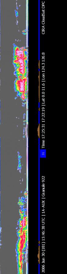
25 19 4. RESULTS Several investigations are conducted using the thin cloud features found by postprocessing the 2B-GEOPROF-Lidar product. First we take a quantitative look at thin cloud frequencies and length scales in four seasons and four latitude bands between June, 2006 and May, We then describe the vertical distribution of thin clouds by length. This is followed by a discussion of the relative contribution of long thin clouds to the total thin cloud fraction and what impacts this might have on climate models. Finally, we discuss the global distribution of thin clouds and very long thin clouds. Examples of long thin clouds are shown in figure 6. This figure shows an alongtrack vertical cross-section of a 1306 km long cloud found at night on June 30, The cloud, whose top ranges from 15 km to 16 km in altitude, overlays a second thin cloud of approximately 800 km in length at about 7 km altitude. These two clouds are located over the Pacific warm pool. The upper cloud is continuous from (12.0 S, E) to (0.5 S, E) with an average thickness of 1.5 km and is similar to the laminar cirrus found during the LITE campaign (Winker and Trepte, 1998), which observed a 2700 km long, 1 km thick cloud. While the upper cloud shown in figure 6 is not the longest cloud seen in our dataset (the longest is ~2900 km), it is a good example of the very long thin clouds found in this study. Another advantage of using active remote sensing observations is that the 807 km mid-level cloud is also observed. If passive measurements were used, this cloud would not be observed as a separate feature.

26 20 Our first investigation will be a quantitative look at cloud length and frequency by location, Tables 1 through 3 show the mean and median cloud lengths and the percentage of area coverage of thin cloud in four latitude bands (0 to 60 S/N; 0 to 20 S/N; 20 S/N to 40 S/N, 40 S/N to 60 S/N) over four seasons for: 1) the troposphere above 3 km, 2) the upper troposphere, and 3) the mid-levels. To prevent the introduction of an observational system bias, only nighttime data is used. Also, so that seasonal differences are more apparent, these tables show data for the northern hemisphere only. Because the data describing the four seasons in Tables 1 through 3 have been computed using only one year of data, discussion is restricted to seasonal differences in More years of data will be necessary before conclusions regarding seasonal variability can be drawn. The right hand column, % Cloudy, is a cloud fraction. To compute this cloud fraction, we first determine which thin clouds are contained in the specific region or season. The number of 2B-GEOPROF-Lidar profiles that each individual cloud traverses is then determined, and the cloud lengths in number of vertical profiles, are summed. This total is then divided by the total number of 2B-GEOPROF-Lidar vertical profiles contained in the corresponding region or season. It should also be noted that when two cloud structures are overlapping, two clouds are counted. As a consequence, the cloud fraction will be higher than if overlapping clouds were counted only once. All three altitude ranges shown in tables 1 through 3 show total cloudiness from thin clouds is highest in the tropical region (0-20 N) regardless of season. This difference in thin cloud coverage is most notable in the upper troposphere where the tropical cloud coverage is close to or more than double that seen in either of the extra-

27 21 tropical latitude bands, regardless of season. The higher amount of thin cloud coverage in the tropics is likely due to convective uplift causing moist air to ascend to the tropical tropopause. As the air moves toward the tropopause, its temperature drops and saturation occurs, allowing clouds to form in the cold trap while upper-level divergence helps to expand the cloud regions in the horizontal. The lower amounts of thin cloud seen in the extra tropics, compared to the tropics, may be due to lower amounts of convective activity and stronger subsidence in the region. Seasonal differences in cloud fraction in all latitude bands are in phase with each other. Thin cloud fraction is highest in the summer season (JJA) and lowest in winter (DJF) in all latitude bands. In the upper troposphere, thin cloud fraction shows the most appreciable seasonal difference in the 20 N-40 N latitude band with 19.1% cloud fraction during the summer season and 4.3% cloud fraction in the winter season. In the 40 N-60 N latitude band, the seasonal differences are also apparent, 19.8% in summer and 10.3% in winter, although smaller in magnitude than in the 20 N-40 N band. While seasonal differences in high thin cloud fraction in the tropical latitudes show a similar pattern, it is difficult to draw conclusions based on the numbers because the change in cloud fraction from summer (39.5%) to winter (35.5%) is small relative to the total cloud fraction. Seasonal differences in average high thin cloud length are in phase with the seasonal differences seen in total thin cloud fraction for both the 0-20 N and 40 N- 60 N latitude bands. The tropical regions show the largest difference in average high thin cloud length with 80.8 km in JJA and km in DJF, a change of over 33% from

28 22 summer to winter. The average high thin cloud length between 20 N and 40 N also shows a large difference between seasons; however, the seasonal differences are out of phase with those found in the other two latitude bands. Between 20N and 40N the average high thin cloud length is shortest in the spring season (62.4 km) and longest in the winter season (88.9 km). In contrast to this, thin cloud length in the mid-troposphere does not change appreciably from season to season. In general, regardless of season or altitude, the average thin cloud is longer in the tropics than in either of the other latitude bands. This difference in cloud length between latitude bands changes with respect to cloud height. Figure 7 depicts three cumulative distribution functions (CDFs) of fraction of thin clouds by cloud length for the northern hemisphere nighttime over the year. These CDFs are created using length bins of 5 km. For each 5 km length range, we determine the total number of thin clouds whose lengths are within or below that length range. These numbers are then divided by the total number of thin clouds giving us the fraction of thin clouds whose lengths are shorter than or equal to a given length. So, for example, if we have a fraction of 0.9 for thin clouds with lengths of 50 km, which tells us that 90% of all thin clouds are shorter than 50 km. To retrieve very optically thin clouds, the CALIPSO cloud mask algorithm uses a spatial averaging technique to reduce signal noise and bring out cloud and aerosol features (McGill et al., 2007). This averaging is performed at three horizontal distances: 5 km, 20 km, and 80 km. The result of this averaging can be seen in the CDFs of cloud length. At 80 km in all three plots, and at 160 km in the upper troposphere CDF, we see

29 23 a jump in cloud fraction. Averaging at 80 km causes a larger number of clouds to appear in the data set as being 80 km long. If these were plotted as PDFs, we would also see spikes at 5 km and 20 km. The CDFs for the troposphere above 3 km or in the mid levels alone (figure 7 a and c) show that there is a tendency towards slightly longer clouds in the tropics than at higher latitudes. As can be seen, though, in figure 7 (a and c) and tables 1 and 3, the difference does not seem to be appreciable in the mid-levels and is relatively small when considering the troposphere above 3 km. When the troposphere above 3 km is considered, the fraction of clouds longer than 200 km ranges from ~5% in the tropics to ~1.5% between 40 N and 60 N, while in the mid levels, these percentages are nearly zero. In the upper levels, the situation is quite different, as can be seen by the greater separation between the lines. Less than 3% of thin clouds seen in the upper levels between 40 N and 60 N are longer than 200 km. In the tropics, however, over 11% of thin clouds seen are longer than 200 km. The change in cloud length from one latitude band to another is greater in the upper troposphere than in the mid troposphere. Figure 8, a histogram, shows thin cloud length versus height for the tropical nighttime troposphere. Note that the contour levels start at 10 and increase by each interval. From this figure, is clear that long, thin clouds are predominantly located at high altitudes, between 13 km and 18 km, with some clouds extending over distances greater than 1000 km. Throughout the mid and lower troposphere, thin clouds tend to be much shorter with few clouds longer than 200 km.

30 24 The general features seen in figure 8 are also apparent in the mid-latitudes. Figures 5 and 6 show histograms of thin cloud length versus height for 20 S/N to 40 S/N and 40 S/N to 60 S/N, respectively. Although, as seen before, extratropical thin clouds tend to be shorter than those found in the tropics, in both latitude bands we see that long clouds are predominantly found near the tropopause. Cloud counts in the midlevels tend to be lower than in the upper levels and those clouds that exist in the mid levels tend to be relatively short. Note also that in all three figures (8-10) we have included the lower troposphere, below 3 km. Thin cloud counts in the lower troposphere are much higher than in the upper and mid-levels. Also, while shorter than the near tropopause clouds, thin clouds in the lower levels tend to be slightly longer than those found in the mid-levels. As noted by Haladay and Stephens (2009), it is uncertain if the higher cloud counts in the lower troposphere are correct or are due to misclassified aerosol and additional signal noise. Cloud counts in the lower troposphere are considerably higher than any other part of the troposphere. The peak cloud counts in figures 8-10 are from clouds around 1 km altitude and less than 50 km in length. These peaks are a full order of magnitude higher than cloud counts in any other length/height regime. When plotted as a histogram by cloud base height (figure 11) we see that ~60% of all low thin cloud found in this data is attributable to clouds with bases below 500 meters and ~80% is due to clouds with bases below 1 km. It is difficult to say for certain, but this low cloud data is likely a product of increased aerosol misclassification by CALIPSO in the lower troposphere. This is the predominant reason that clouds below 3 km are omitted for much of this study.

31 25 Figures 8-10 suggest that long thin clouds constitute a large portion of the total area coverage from thin clouds in the upper troposphere while in the mid-latitudes and mid-troposphere, they make a negligible contribution. If a large fraction of all thin clouds is contained in long thin clouds, it could have significant implications for parameterization of thin clouds in climate models. Table 4 shows the percent of total thin cloud area contained within clouds longer than 100 km, 200 km, and 500 km for the troposphere above 3 km, the upper levels, and the mid levels. This is computed by summing the lengths of all thin clouds and of thin clouds that are longer than 100 km, 200 km, and 500 km, giving us four different totals. The three totals for long clouds are then divided by the sum of all thin cloud lengths giving us the fraction of all thin cloud that is contained in long thin clouds. In the upper levels over 20% of the total cloud area is contained in clouds longer than 500 km in both the 0 to 20 S/N and the 20 S/N to 40 S/N latitude ranges. Additionally, clouds longer than 100 km contribute over 65% to the total area coverage of thin cloud in both latitude ranges. In the higher latitudes, these numbers decrease. Only 5.62% of cloud area is contained in clouds longer than 500 km between 40S(N) and 60S(N). In the mid-levels, a negligible fraction of cloud area is contributed by clouds longer than 500 km and only about 10% of the total thin cloud area is contained in clouds longer than 100 km. Figures 12 through 15 summarize these results. These figures show the locations of upper-level thin clouds found in JJA, SON, DJF, and MAM respectively. Every twentieth cloud is plotted from each season, both day and night over the whole globe. Clouds shorter than 100 km are denoted simply by a line, while clouds longer than 100

32 26 km are denoted by a line with a symbol placed in the middle. Triangles denote clouds longer than 100 km, squares are clouds longer than 200 km, and diamonds are clouds longer than 500 km. In all four seasons, we see a maximum in thin cloud coverage between 30S and 30N with minima in the mid-latitudes and secondary maxima in the high latitudes. Most of the long clouds are concentrated in the tropics, with some in the high latitude maxima. The difference in long cloud amount between the tropical and extra-tropical maxima is likely due to the relative frequencies of convection and relative availability of moisture in the two regions, while the mid-latitude minima are likely due to subsidence. Thin clouds appear to follow the inter-tropical convergence zone and the midlatitude storm tracks as also shown by Dessler et al. (2006) and Wylie and Menzel (1999). If we were to draw a line of best fit through the clouds in the tropics in figure 12, we would see that the average cloud is located at about 12 N during northern hemisphere (NH) summer. As we progress into the NH fall season, line of best fit drops to approximately the equator. In the NH winter season, the average thin cloud moves to about 9S then returns to the equator in the NH spring season. This lends some backing to the theory that these clouds are predominately formed by convective activity. The mid-latitude minima are strongest in each hemisphere s respective winter. Very few thin clouds are found between 25 S and 50 S in the southern winter season or between 30 N and 50 N in the northern winter season. The north-south temperature gradient in the winter hemisphere sets up large-scale subsidence in these regions, reducing the lifetimes of high thin clouds by drawing them to lower, warmer altitudes

33 27 and breaking them up through turbulence. In contrast, during the summer season in each hemisphere, thin cloud amounts in these regions are higher, except in the location of the mid-latitude highs. This is probably because the reduced north-south temperature gradient in summer causes reduced subsidence and therefore allows clouds to reside, undisturbed, in the upper levels for longer time periods. Before concluding, we will point out a few final interesting features. In figure 12, we see the tropical thin cloud coverage maximum extend well into the Indian subcontinent. This is probably due to the Indian monsoon. Also, when we compare figure 13 to figures 12 and 14, we see an increase in cloud coverage across the Atlantic. It is possible that this is due to increased tropical storm activity during September and October 2006.

34 28 5. CONCLUSIONS Thin cloud length scales, locations, vertical distributions, and seasonal differences are determined in this study. We also determine the contribution of long thin clouds to the total thin cloud fraction. Due to their low optical depth, observation of thin clouds has traditionally been difficult using satellites and human observations. As such, much less is known about their size and shape than is known for other cloud types. Determining their horizontal scales is important for understanding how they form and how they effect different atmospheric and climatic processes such as: climate change through their greenhouse effect, stratospheric dehydration (Hartmann et al., 2001; Immler et al., 2008), and the evolution of underlying cloud structures (Garrett et al., 2006). Understanding the length scales of thin clouds may also prove useful in developing more accurate cloud parameterizations for climate models. Using a post-processing algorithm and nearly one year of data from the 2B- GEOPROF-Lidar product (Mace et al., 2009), we piece together horizontally continuous thin clouds as found along the tracks of CloudSat and CALIPSO. Clouds are considered thin if they are seen by CALIPSO, but not detected by CloudSat. Based on estimates from Haladay and Stephens (2009), this corresponds to a visible optical depth range of 0.02 to 0.3 with an average optical depth of 0.1. To eliminate a possible strong day/night bias in the CALIPSO observations, only nighttime data is used for this study. Also, because some uncertainty exists about whether the low level thin cloud seen in the

35 29 data has been correctly classified (Haladay and Stephens, 2009), no data below 3 km is utilized, except where indicated. For this study, a horizontally continuous cloud is composed of a set of consecutive measurements that contain cloud in some of the same vertical levels. For example, if cloud is found in one measurement profile between 10 km and 12 km and cloud is found in the following measurement profile between 11 km and 13 km, the two cloud layers are considered parts of the same cloud. Cloud layers in the same measurement profile are only considered to be separate cloud layers if they vertically separated by more than 1 km. Also, the post-processing algorithm can handle no more than two overlapping clouds at a time. If three thin cloud layers with separations of more than 1 km are found, the two closest layers are combined. If more than three thin clouds layers are found, the lowest cloud is removed since it will have the lowest radiative impact. Situations with more than three thin cloud layers occur less than 0.005% of the time. Analyses of the thin clouds found using our post-processing algorithm show that thin clouds are predominantly found in the tropical upper troposphere, but do occur throughout the troposphere and across the globe. In the tropics the thin cloud fraction is approximately 68% with over half (38% cloud fraction) of those thin clouds found in the upper troposphere. Between 20S(N) and 40S(N) the total tropospheric thin cloud fraction is about 34%, about a third of which (10% cloud fraction) are found in the upper troposphere. The 40S(N) to 60S(N) latitude band contains the least thin cloud, about 27% total tropospheric thin cloud fraction, with 15% upper tropospheric thin cloud

36 30 fraction. Thin clouds occur about 33.5% of the time between 20 S/N and 40 S/N with about 10% cloud fraction in the mid-latitude upper troposphere and about 29% of the time between 40 S/N and 60 S/N with about 15% cloud fraction in the upper troposphere. Average cloud lengths are found to be dependent on cloud height, latitude, and season. The average northern hemisphere thin cloud is about 34 km in length, while the average thin cloud in the northern hemisphere tropics is longer, about 47 km. The longest thin clouds found in the northern hemisphere tend to be located in the tropical upper troposphere and range from about 81 km in the northern hemisphere summer to over 108 km in the northern hemisphere winter. Although, shorter on average, extratropical thin cloud lengths vary in phase with those in the tropics with the shortest thin clouds in local summer and the longest thin clouds in local winter. In all regions of the troposphere thin cloud counts are dominated by short thin clouds. Even so, long thin clouds constitute a large percentage of the total thin cloud fraction in the upper troposphere. Over 20% of the total thin cloud fraction in the upper troposphere is contributed by thin clouds that are longer than 500 km between 0 and 40 N. In fact, in this latitude range, over 65% of the total cloud fraction due to thin clouds is contributed by clouds longer than 100 km. The large contribution by long clouds to the total thin cloud fraction could have impacts on how thin clouds are modeled in GCM. GCM grid resolutions can range from as large as a few hundred kilometers down to a few tens of kilometers. This grid spacing makes it difficult to resolve many cloud features as they tend to be smaller than the grid

37 31 boxes. As such, sub-grid parameterizations are required to produce realistic distributions for cloud features in GCM. The long thin clouds found in this study, however, would cover multiple grid boxes and it may be possible to model them at the native resolution of GCM. On the other hand, realistic modeling of shorter thin clouds, which dominate the total number of thin clouds, would still, require a sub-grid parameterization. Thin clouds, especially long thin clouds, are associated with convectively active regions. High concentrations of thin cloud occur over the Pacific warm pool, equatorial Africa and South America, along the ITCZ, and in the mid-latitude storm tracks. Very little thin cloud is found in non-convective regions, such as the mid-latitude highs and zones of large-scale subsidence. Additionally, the long thin clouds are predominantly located over the ITCZ with a smaller number over the mid-latitude storm tracks. Even when thin clouds are found in non-convectively active regions, they tend to be short. The high percentage of total cloud fraction contained in long clouds in the tropical upper troposphere and the radiative importance of high, cold, thin clouds, suggest that long thin clouds play a major role in global climate and local meteorology. Their large area allows them to slow the diffusion rate of anvil cirrus over large regions, diminishing their effect on local climate. Also, their prevalence, and extent may allow for widespread dehydration of air entering the stratosphere from the troposphere.

38 32 REFERENCES Brunner, D., P. Siegmund, P. T. May, L. Chappel, C. Schiller, R. Muller, T. Peter, S. Fueglistaler, A. R. MacKenzie, A. Fix, H. Schlager, G. Allen, A. M. Fjaeraa, M. Streibel, and N. R. P. Harris, 2009: The SCOUT-O3 Darwin aircraft campaign: Rationale and meteorology, Atmos. Chem. Phys., 9, Chen, Y., and A. D. Del Genio, 2009: Evalutation of tropical cloud regimes in observations and a general circulation model, Clim. Dyn., 32, , doi: /s Dessler, A. E., S.P. Palm, W. D. Hart, and J. D. Spinhirne, 2006: Tropopause-level thin cirrus coverage revealed by ICESat/Geoscience Laser Altimeter System, J. Geophys. Res., 111, D08203, doi: /2005jd Febvre, G., J. G. Gayet, A. Minikin, H. Schlager, V. Shcherbakov, O. Jourdan, R. Busen, M. Fiebig, B. Karcher, and U. Schumann, 2009: On optical and microphysical characteristics of contrails and cirrus, J. Geophys. Res., 114, D02204, doi: /2008jd Fueglistaler, S., M. Bonazzola, P. H. Haynes, T. Peter, 2005: Stratospheric water vapor predicted from the Lagrangian temperature history of air entering the stratosphere in the tropics, J Geophys. Res., 110, D08107, doi: /2004jd Garrett, T. J., A. J. Heymsfield, M. J. McGill, B. A. Ridley, D. G. Baumgardner, T. P. Bui, and C. R. Webster, 2004: Convective generation of cirrus near the tropopause, J. Geophys. Res., 109, D21203, doi: /2004jd Garrett, T. J., M. A. Zulauf, and S. K. Krueger, 2006: Effects of cirrus near the tropopause on anvil cirrus dynamics, Geophys. Res. Lett., 33, L17804, doi: /2006gl Haladay, T., and G. Stephens, 2009: Characteristics of tropical thin cirrus clouds deduced from joint CloudSat and CALIPSO observations, J. Geophys Res, doi: /2008jd010675, in press. Hartmann, D. L., J. R. Holton, and Q. Fu, 2001: The heat balance of the tropical tropopause, cirrus, and stratospheric dehydration, Geophys. Res. Lett., 28, Hogan, R. J., A. J. Illingworth, 2000: Deriving cloud overlap statistics from radar: Q. J. R. Meteor. Soc., 126,

39 33 Immler, F., K. Kruger, S. Tegtmeier, M. Fujiwara, P. Fortuin, G. Verver, O. Schrems, 2007: Cirrus clouds, humidity, and dehydration in the tropical tropopause layer observed at Paramaribo, Suriname (5.8N, 55.2W), J. Geophys. Res., 112, D03209, doi: /2006jd ,, M. Fujiwara, G. Verver, M. Rex, and O. Schrems, 2008: Correlation between equatorial Kelvin waves and the occurrence of extremely thin ice clouds at the tropical tropopause, Atmos. Chem. Phys., 8, Kim, S. W., S. Berthier, J. C. Raut, P. Chazette, F. Dulac, and S. C. Yoon, 2008: Validation of aerosol and cloud layer structures from the space-borne lidar CALIOP using a ground-based lidar in Seoul, Korea, Atmos. Chem. Phys., 8, Kumar, S. V. S., K. Parameswaran, B. V. K. Murthy, 2003: Lidar observations of cirrus cloud near the tropical tropopause: General features, Atmos. Res., 66, Larson, V. E., R. Wood, P. R. Field, J. Golaz, T. H. Vonder Haar, W. R. Cotton, 2001: Systematic biases in the microphysics and thermodynamics of numerical models that ignore subgrid-scale variability, J. Atmos. Met. Soc, 58, Liou, K. N., 1986: Influence of cirrus clouds on weather and climate processes, Mon Weather Rev., 114, Mace, G.G., R. Marchand, and G. L. Stephens, 2007: Global hydrometeor occurrence as observed by CloudSat: Initial observations from summer 2006, Geophys. Res. Lett., 34, L09808, doi: /2006gl , Q. Zhang, M. Vaughn, R. Marchand, G. Stephens, C. Trepte, and D. Winker, 2009: A description of Hydrometeor layer occurrence statistics derived from the first year of merged CloudSat and Calypso data, J. Geophys. Res., doi: /2008jd Marchand, R., G. G. Mace, T. Ackerman, G. Stephens, 2008: Hydrometeor detection using CloudSat An earth-observing 94 GHz cloud radar, J. Atmos. Ocea. Tech., 25, , J. Haynes, G. G. Mace, T. Ackerman, and G. Stephens, 2009: A comparison of simulated cloud radar output from the multiscale modeling framework global climate model with CloudSat cloud radar observations, J. Geophys. Res., 114, D00A20, doi: /2008jd McGill, M. J., M. A. Vaughan, C. R. Trepte, W. D. Hart, D. L. Hlavka, D. M. Winker, and R. Kuehn, 2007: Airborne validation of spatial properties measured by the CALIPSO lidar, J. Geophys. Res., 112, D20201, doi: /2007jd

40 34 Nasiri, S. L., and B. A. Baum, 2004: Daytime multilayered cloud detection using multispectral imager data, J. Atmos. Ocea. Tech., 21, , Pace, G., M. Cacciana, A. di Sarra, G. Fiocco, and D. Fua, 2003: Lidar observations of equatorial cirrus clouds at Mahe Seyehelles, J. Geophys. Res., 108, 4236, doi: /2002jd Randall, D. A., R. A. Wood, S. Bony, R. Colman, T. Fichefet, J. Fyfe, V. Kattsov, A. Pitman, J. Shukla, J. Srinivasan, R. J. Stouffer, A. Sumi, and K. E. Taylor, 2007: Climate Models and Their Evaluation. Climate Change 2007: The Physical Basis. Contribution of Working Group I to the Fourth Assessment Report of the Intergovernmental Panel on Climate Change, S. Solomon, D. Qin, M. Manning, Z. Chen, M. Marquis, K. B. Averyt, M. Tignor, and H. L. Miller, Eds., Cambridge University Press. Rossow, W. B., R. A. Schiffer, 1999: Advances in understanding clouds from ISCCP, Bull. Amer. Met. Soc., 80, Sassen, K., 2002: Cirrus clouds: A modern persepctive, Cirrus, D. Lynch, K. Sassen, D. O C. Starr, and G. L. Stephens, Eds, Oxford Univ. Press, Spinhirne, J. D., W. D. Hard, and D. L. Hlavka, 1996: Cirrus infrared parameters and shortwave reflectance relations from observations, J. Atmos. Sci., 53, Stephens, G. L., S. C. Tsay, P. W. Stackhouse, and P. J. Flatau, 1990: The relevance of the microphysical and radiative properties of cirrus clouds to climate and climatic feedback, J. Atmos. Sci., 47, , D. G. Vane, R. J. Boain, G. G. Mace, K. Sassen, Z. Wang, A. J. Illingsworth, E. J. O Connor, W. B. Rossow, S. L. Durden, S. D. Miller, R. T. Austin, A. Benedetti, C. Mitrescu, and the CloudSat Science Team, 2002: The CloudSat Mission and the A- Train: A new dimension of space-based observations of clouds and precipitation, Bull. Amer. Met. Soc., 83, , D. G. Vane, S. Tanelli, E. Im, S. Durden, M. Rokey, D. Reinke, P. Partian, G. G. Mace, R. Austin, T. L Ecuyer, J. Haynes, M. Lebsock, K. Suzuki, D. Waliser, D. Wu, J. Kay, A. Gettelman, Z. Wang, and R. Marchand, 2008: CloudSat mission: Performance and early science after the first year of operation, J. Geophys. Res., 113, D00A18, doi: /2008JD Vaughan, M., S. Young, D. Winker, K. Powell, A. Omar, Z. Liu, Y. Hu, and C. Hostetler, 2004: Fully automated analysis of space-based lidar data: An overview of the CALIPSO retrieval algorithms and data products, Proc. SPIE, 5575,

41 35 Wang, L. K., and A. E. Dessler, 2006: Instantaneous cloud overlap statistics in the tropical area revealed by ICESat/GLAS data, Geophys. Res. Lett., 33, L15804, doi: /2005gl Willén, U., S. Crewell, H. K. Baltink, O. Sievers, 2005: Assessing model predicted vertical cloud structure and cloud overlap with radar and lidar ceilometer observations for the Baltex Bridge Campaign of CLIWA-NET, Atmos. Res., 75, Winker, D. M. and C. R. Trepte, 1998: Laminar cirrus observed near the tropical tropopause by LITE, Geophys. Res. Lett., 25, , W. H. Hunt, and M. J. McGill, 2007: Initial performance assessment of CALIOP, Geophys. Res. Lett., 34, L19803, doi: /2007gl

42 36 APPENDIX A FIGURES AND TABLES

43 37

44 Figure 2: An example of data as seen by CALIPSO. This image is a quicklook image from The data are from June 30, 2006 between 18:49:02 and 10:02:37 UTC. 38

45 Figure 3: Depicts the altitude ranges used in the post-processing algorithm. The third altitude range, troposphere above 3 km covers the area between the line at 3 km and the top of the high altitude range. 39

46 Figure 4: A set of hypothetical cloud profiles. Each hypothetical profile contains cloud, denoted by a vertical line. A dashed box surrounds each set of cloud layers that the algorithm would consider to be part of the same cloud. The 3 km cloud length and the 3 km gap length assumptions are ignored for this plot. 40

47 Figure 5: Flow chart describing the post-processing algorithm. Note, only the case where one cloud layer is found per profile is described here. The algorithm is much more complicated for two or more cloud layers. 41

48 Figure 6: Depiction of a 1306 km long cloud overlaying an 807 km cloud. The upper cloud extends from (12.5 S, E) to (0.5 S, E) and has an average thickness of 1.5 km. Both clouds are seen only by CALIPSO. 42

49 Figure 7: Cumulative distribution functions of nighttime thin cloud length for (a) the troposphere above 3 km, (b) the upper troposphere, and (c) the mid-troposphere. Four latitude bands are presented for each height range: 0 to 60 (solid), 0 to 20 (dotted), 40 to 60 (dash dot). Each latitude band includes data from both hemispheres. 43

50 Figure 8: Histogram of thin cloud count by cloud top height and cloud length for the tropical (20 S to 20 N) nighttime. Bins are 1 km height by 50 km length. 44

51 Figure 9: Same as figure 8 but for 20 S(N) to 40 S(N). 45

52 Figure 10: Same as figure 8 but for 40 S(N) to 60 S(N). 46

53 Figure 11: Histogram of thin cloud base heights by percent of total thin cloud count. Bin size is 100 km length. 47

54 Figure 12: Thin cloud locations for thin clouds found in June, July, and August Individual lines represent individual clouds. Lines without symbols are less than 100 km in length. All other cloud lengths are denoted by symbols in the middle of their line. Triangles are clouds longer than 100 km, squares are clouds longer than 200 km, and diamonds are cloud longer than 500 km in length. Every 20 th cloud is plotted. 48

55 Figure 13: Same as figure 12, but for September, October, and November

56 Figure 14: Same as figure 12, but for December, January, and February 2006/

57 Figure 15: Same as figure 12, but for March, April, and May