Marchand et al. 2008, Comparison of MMF with CloudSat Accepted JGR 05/2008 p. 1. A Comparison of Simulated Cloud Radar Output

Transcription

1 Marchand et al. 2008, Comparison of MMF with CloudSat Accepted JGR 05/2008 p. 1 A Comparison of Simulated Cloud Radar Output from the Multiscale Modeling Framework Global Climate Model with CloudSat Cloud Radar Observations Roger Marchand 1, John Haynes 2, Gerald G. Mace 3, Thomas Ackerman 1, Graeme Stephens 2 1. Joint Institute for the Study of the Atmosphere and Ocean, University of Washington 2. Department of Atmospheric Sciences, Colorado State University 3. Department of Meteorology, University of Utah

2 Marchand et al. 2008, Comparison of MMF with CloudSat Accepted JGR 05/2008 p. 2 Abstract Over the last few years a new type of global climate model (GCM) has emerged in which a cloud-resolving model (CRM) is embedded into each grid cell of a GCM. This new approach is frequently called a Multiscale Modeling Framework (MMF) or superparameterization. In this article we present a comparison of MMF output with radar observations from the NASA CloudSat mission, which uses a near nadir-pointing millimeter-wavelength radar to probe the vertical structure of clouds and precipitation. We account for radar detection limits by simulating the 94 GHz radar reflectivity that CloudSat would observe from the high-resolution cloud-resolving model output produced by the MMF. Overall the MMF model does a good job of reproducing the broad pattern of tropical convergence zones, subtropical belts, and mid-latitude storm tracks, as well as, their changes in position with the annual solar cycle. Nonetheless, the comparison also reveals a number of model shortfalls including: (1) Excessive hydrometeor coverage at all altitudes over many convectively active regions. (2) A lack of low-level hydrometeors over all subtropical oceanic basins. (3) Excessive low-level hydrometeor coverage (principally precipitating hydrometeors) in the mid-latitude storm tracks of both hemispheres during the summer season (in each hemisphere). (4) The MMF also has a thin band of low-level hydrometeors in the southern hemisphere of the central (and at times eastern and western) Pacific, which is not observed by CloudSat. This band resembles a second much weaker ITCZ, but is restricted to low levels.

3 Marchand et al. 2008, Comparison of MMF with CloudSat Accepted JGR 05/2008 p Introduction Over the last few years a new type of global climate model (GCM) has emerged in which a two-dimensional or small three-dimensional cloud-resolving model (CRM) is embedded into each grid cell of a GCM. The embedded CRM removes the need for most of the cloud parameterizations used in traditional GCMs. This new approach is frequently called a Multiscale Modeling Framework (MMF), but is also known as a cloud-resolving convection parameterization or a superparameterization (Grabowski 2001, Randall et al. 2003). The MMF has been the focus of several evaluation studies including Khairoutdinov and Randall (2001), Khairoutdinov et al. (2005), Marchand et al. (2005), Ovtchinnikov et al. (2006), DeMott et al. (2007), and McFarlane et al (2007). In this article, we extend the above evaluation studies to include a comparison of MMF output with observations from CloudSat (Stephens et al. 2002). Launched in late April 2006, CloudSat uses a near nadir-pointing millimeterwavelength radar to probe the vertical structure of clouds and precipitation, which we will collectively refer to as hydrometeors. The CloudSat radar does not scan, but generates a curtain or two-dimensional cross section through the atmosphere as the satellite moves along its orbital trajectory. The radar transmits pulses with an approximate duration of 3.3 μs, and so measures hydrometeor reflectivity with an effective vertical range resolution of approximately 480 m. However, the measured return power is sampled at a rate equivalent to about 240 m in range (that is, the measured data are two times over sampled). Pulses are averaged about 0.16 s along the nadir track yielding an effective footprint (6 db) at the surface of about km for each radar profile. The minimum detectable signal from the CloudSat radar is slightly

4 Marchand et al. 2008, Comparison of MMF with CloudSat Accepted JGR 05/2008 p. 4 exceeding expectations with sensitivity of about -30 dbz throughout the troposphere (Tanelli et al., 2008). This combination of sensitivity and resolution is not sufficient to detect many clouds (Stephens et al. 2002, Marchand et al. 2007). It is therefore critical when comparing CloudSat observations (or retrievals) with model output to account for the radar limitations. In this study, we account for the radar detection capabilities by simulating the 94 GHz radar reflectivity that CloudSat would observe from the highresolution cloud-resolving model output produced by the MMF. We then compare statistical summaries of the actual CloudSat observations with those simulated from the model output and include only those model hydrometeors which CloudSat can detect. We stress that the radar penetrates all cloud and most precipitation, and the vertical structure shown here is not the distribution of cloud top - as is often estimated from passive visible or infrared imagers, e.g. by the International Satellite Cloud Climatology Project (ISCCP). In sections 2 and 3 of the paper we describe the MMF model and the radar simulator, respectively. Then in section 4 we contrast vertically resolved hydrometeor fractional coverage (that is, vertical profiles of hydrometeor occurrence) and twodimensional histograms of radar reflectivity with height from CloudSat and the model. Finally, we summarize the results in section The Multiscale Modeling Framework (MMF) This study uses the MMF as developed by Khairoutdinov and Randall at Colorado State University. It consists of the NCAR CAM and an embedded 2D cloud resolving

5 Marchand et al. 2008, Comparison of MMF with CloudSat Accepted JGR 05/2008 p. 5 model. The details of the MMF configuration are given by Khairoutdinov and Randall (2001) and Khairoutdinov et al. (2005) and are only briefly described here. The NCAR Community Atmosphere Model (CAM 3.0) is the atmospheric component of the Community Climate System Model (CCSM). In our version of the MMF, CAM is run with the finite volume dynamical core and has 26 vertical layers and a horizontal resolution of 2 o latitude and 2.5 o longitude. The dynamical time step of the CAM is 20 minutes. Details of the CAM physics can be found in Collins et al. (2004, 2006) and Boville et al. (2006). The embedded CRM (Khairoutdinov and Randall 2003) within each CAM grid cell has 64 columns at 4 km spacing and 24 layers in the vertical, which coincide with the lowest 24 levels of the CAM. The CRM domain is aligned in the eastwest direction with cyclic lateral boundary conditions. The CRM runs continuously with its own 15 to 20 second dynamical time step. Radiation calculations using the CAM radiative transfer code are performed on each CRM column every 10 minutes. The CRM predicts the total non-precipitating water (vapor + liquid + ice) and total precipitating water (rain + snow + graupel). The CRM uses the same optical property parameterizations and radiation code as the CAM, although no overlap approximation is needed. The MMF simulation was initialized on 1 September 1997 using initial model fields from a CAM spinup simulation and was run through June 2002, using observed monthly sea surface temperatures (SST). We note that the MMF data used here are not subsampled to reproduce the orbital characteristic of CloudSat, but rather includes observations from all times of day. In the future we also plan to output model data to support such sub-sampling, and to study quantitatively the effect such sampling may introduce in the monthly means.

6 Marchand et al. 2008, Comparison of MMF with CloudSat Accepted JGR 05/2008 p Description of Radar Simulator and CloudSat GeoProf data Radar returns were simulated from the model output using the QuickBeam radar simulation package (Haynes et al. 2007). QuickBeam takes vertical profiles of cloud and precipitation mixing ratios produced by a cloud resolving model and converts them into equivalent radar reflectivities as would be viewed from a satellite passing over the model domain or from a ground based radar. In the current version of this software (V1.04) all particles are assumed to be spherical and scattering is treating using Mie theory. Studies by Lemke and Quante (1999) and Sato and Okamoto (2006) show the maximum difference in radar reflectivity between that obtained using a full electromagnetic solver (e.g., the discrete dipole approach) and Mie theory (using equivalent volume spheres) is less than 1.2 db for r eff 100 μm and less than 4 db for 100 μm r eff 600 μm, where r eff is the radius of the equivalent volume sphere. While the scattering is treated using Mie theory, QuickBeam allows the density of the frozen particles to be specified using a mass-to-diameter power-law relationship. Lookup tables are used to decrease computation time, and have been designed to produce errors of less than 1.2 dbze when compared with explicit Mie calculations. Attenuation by the particles is calculated (again from Mie theory) and gaseous attenuation by water vapor and oxygen (which is non-negligible at 94 GHz) is treated using the method of Liebe (1985), which is accurate to better than 0.5 dbze. It is also assumed that multiple scattering effects are negligible. Multiple scattering acts to increase the apparent observed reflectivity below regions with large attenuation. For CloudSat, multiple scattering is typically not significant except for rain

7 Marchand et al. 2008, Comparison of MMF with CloudSat Accepted JGR 05/2008 p. 7 exceeding approximately 3 mm hr 1 (Battaglia et al 2007, 2008). While an important issue for rain-rate and microphysical retrievals, in the present analysis where we are largely examining hydrometeor occurrence rates the effect of multiple scattering is expected to be small. In general, we expect multiple scattering will tend to slightly increase the observed occurrence rate due to false detections in places where highly attenuating hydrometeor occur above regions devoid of any hydrometeors. This can happen, for example, when hydrometeors forming at the melting layer have yet to fall sufficiently far to fill the space between the formation level and the surface. We expect such to occur only a small fraction of the time, and as we shall see in the next section, the model tends to overestimate rather than underestimate the hydrometeor occurrence rates and reflectivity relative to observations. QuickBeam allows the user to represent hydrometeors using a number of distribution models including exponential, lognormal, modified gamma, power law, and monodispersed. A separate distribution model can be selected for each hydrometeor type predicted by the cloud resolving model. Each of these distributions has two or three degrees of freedom (that is, two or three parameters are needed to fully define the distribution and there are variety of parameters set options that one can select). QuickBeam uses the ice or liquid water content and the other one or two parameters must be specified in a way that is consistent with the model microphysical scheme. The CRM embedded in the MMF is called SAM, the System for Atmospheric Modeling, and uses a bulk microphysics scheme in which the conversion rates among precipitating model hydrometeors are parameterized assuming that the drop size distribution follows a Marshall Palmer or exponential distribution,

8 Marchand et al. 2008, Comparison of MMF with CloudSat Accepted JGR 05/2008 p. 8 n( D) = N o exp( λd). πn Where, = o ρ λ I 1 4, I = ice water content, ρ = hydrometer density, and N o is the socalled intercept parameter and is assumed to have a fixed value 8x10 6 m -4 for rain and 3x10 6 m -4 for snow and graupel. The CRM does not make an explicit assumption for the distribution of nonprecipitating liquid or water ice. However, the CRM uses the CAM radiation scheme, which sets the effective radius. Over ocean and sea ice, the cloud drop effective radius for liquid water clouds is fixed at 14 μm, while over land the effective radius varies from 8 to 14 μm depending on the temperature (Boville et al. 2006). Ice particle effective radius is defined solely as a function of temperature (Boville et al. 2006, Kristjansson et al. 2000). To be consistent with the radiation scheme, we use the same effective radius as used in the radiation scheme and assume a log-normal distribution for water and a 2 nd order gamma distribution for ice. (The order of the distribution has little effect on the radar reflectivity for a given ice water content and effective radius.) It should be noted that while we use the radar simulator to estimate the 94 GHz reflectivities, as they would be observed from space with CloudSat like resolution, the Quickbeam simulator can be used to estimate the reflectivity from ground-based platforms and lower frequencies radars such as the 35 GHz systems used by the U.S. Department of Energy Atmospheric Radiation Measurement (ARM) program or the 14 GHz system used by the NASA Tropical Rainfall Measurement Mission (TRMM). The CloudSat observations come from the operational CloudSat Geometric Profile dataset, known as 2B-GeoProf or simply GeoProf. This dataset is organized such

9 Marchand et al. 2008, Comparison of MMF with CloudSat Accepted JGR 05/2008 p. 9 that there is one-file per orbit, and in the NASA nomenclature such data are referred to as level 2 products. (The B in 2B is internal to the CloudSat project and indicates that this data product can be used as input to stage C algorithms). GeoProf contains a hydrometeor detection mask which has a value between 0 and 40 for each radar resolution volume. Values greater than 5 indicate the location of likely hydrometeors, with increasing values indicating a reduced probability of a false detection. In addition to the hydrometeor mask, this product contains the radar reflectivity (i.e., the calibrated measured return power) and an estimate of gas absorption due to oxygen and water vapor on the observed reflectivity (which is not used here because the radar simulator accounts for this absorption). In the results presented here, we have aggregated the GeoProf data on a monthly or seasonal basis. Further details on GeoProf data, including a detailed description of the hydrometeor detection algorithm, can be found in Marchand et al. (2007). 4. Global Patterns Millimeter-wavelength cloud radars, such as CloudSat, are able to penetrate clouds and most rain and are able to produce range resolved measurements of hydrometeor coverage (within the radar sensitivity limit). Figure 1 (left column) shows the global zonal seasonal profile of hydrometeor fraction with height for the first 12 months of CloudSat operation, starting in June 2006 and ending in May The top row shows December, January and February (DJF), below which are plots for March, April, May (MAM); June, July, August (JJA); and September, October, and November (SON). By hydrometeor fraction, we mean the number of observations (at the specified altitude and

10 Marchand et al. 2008, Comparison of MMF with CloudSat Accepted JGR 05/2008 p. 10 latitude) where a cloud or other hydrometeor is detected relative to the number of observations. The hydrometeor fraction is determined from the CloudSat operational hydrometeor detection mask (usually called the cloud mask even though it includes detections of both clouds and precipitation), as described in detail by Marchand et al. (2007). In this paper, only hydrometeors with a reflectivity of dbze or larger were used in determining this fraction. This threshold ensures we only include hydrometeors which can be detected by CloudSat with a low probability of false or failed detection. The middle column of Figure 1 shows the same quantity obtained from the MMF using the radar simulator (described in section 3), except that the model output was averaged over a four-year span from 1998 to The variations in the model output from year to year (not shown) are relatively subtle compared to the difference between the model and observations, as shown in the third column and discussed in this section. We have also compared CloudSat observations for July 2006 with July 2007 and January 2007 with January 2008 (not shown). The CloudSat observations in each year are also more similar to each other than either is to the simulations. Our further discussion focuses in turn on the tropics, subtropics, and extratropics. (a) Tropics Perhaps the most striking feature of the zonal plots is the inter-tropical convergence zone (ITCZ) and the associated downward branches of the Hadley Circulation over the subtropics. During the northern hemisphere summer (JJA) and fall (SON), the CloudSat observations show a vigorous ITCZ located in the northern hemisphere. The observed ITCZ hydrometer fraction is largest in June and July after which it decreases. The model

11 Marchand et al. 2008, Comparison of MMF with CloudSat Accepted JGR 05/2008 p. 11 shows a similar ITCZ in the northern hemisphere but with hydrometeor fractions that are much larger than observed and with maximum fractional coverage in August rather than June or July (not shown). In November, the ITCZ in the model dramatically weakens to the point where the hydrometeor coverage in the northern hemisphere tropical mid and upper troposphere is actually less than that observed by CloudSat, when zonally averaged (not shown). Both the model and observations also begin to show the emergence of a peak in tropical upper tropospheric hydrometeors in the southern hemisphere during November. Examination of monthly CloudSat observations reveals a gradual increase in upper tropospheric hydrometeor fraction in the southern hemisphere equatorial region, starting in November and extending through April, with a peak in coverage in February and March. The MMF reproduces the general trend in southern hemisphere upper tropospheric clouds, but as is evident if figure 1, the total hydrometeor fractions are too large, the peak is too wide and extends lower in altitude by several kilometers. The CloudSat observations also show that the peak coverage in upper tropospheric hydrometeors in the southern hemisphere during DJF and MAM is less than that of upper tropospheric hydrometeors in the northern hemisphere during JJA or SON; and in MAM, CloudSat observes a symmetric and relatively weak ITCZ in both hemispheres. Overall, the MMF does a good job in capturing these trends. By May both CloudSat and the model show that the northern hemisphere ITCZ is reestablished, but as is the case in JJA the model hydrometeor coverage is too large. Figures 2-4 show the global geographic distribution of peak hydrometeor fraction in three altitude ranges: high (7 to 20 km), mid (3 to 7 km), and low (1.2 to 3 km),

12 Marchand et al. 2008, Comparison of MMF with CloudSat Accepted JGR 05/2008 p. 12 respectively. By peak hydrometeor fraction, we mean the hydrometeor fraction at the altitude (within the specified range) where the MMF hydrometeor profile has its largest value. The CloudSat observations in these figures are taken at the altitude where the MMF peak is located. The left column in figures 2 through 4 shows the CloudSat observations and the middle column shows the model output via radar simulation. Here the CloudSat observations have been aggregated onto a fixed 4 by 4 degree grid. Even at this horizontal and seasonal scale, the CloudSat dataset is rather noisy. The geographical distribution of hydrometeors in the model is broadly similar to that observed by CloudSat. The large overestimate in northern hemisphere ITCZ fractional coverage in JJA and SON (discussed above in connection with Figure 1) is largely focused in the Asian Monsoon region (encompassing Southeast Asia, the Bay of Bengal, India, the Philippines and the western most Tropical Pacific in the northern hemisphere). This is perhaps best seen at high altitudes, Figure 2, but is also evident at mid and low levels (Figures 3 and 4). CloudSat observes the Asian Monsoon region to be active, just not as active as in the model, except possibly in June (not shown). This version of the MMF is known to be convectively over active, producing too much rainfall and too little outgoing longwave flux over this region (Khairoutdinov et al. 2005, DeMott et al. 2007). While the CloudSat observations show a decrease in upper tropospheric hydrometeor fractions from June through August (not shown), the MMF fractional coverage increases, and only begins to decrease in October. In much of the northern hemisphere summer, the model also shows larger than observed hydrometeor fractions along the ITCZ in the central and eastern Pacific. This is most noticeable at low (Figure 4) and mid levels (Figure 3) for JJA. Interestingly, the

13 Marchand et al. 2008, Comparison of MMF with CloudSat Accepted JGR 05/2008 p. 13 model also shows a thin band of hydrometeors at low levels (1.2 to 3 km range) in the southern hemisphere of the central (and at times eastern and western) Pacific. This thin band is more apparent on monthly plots (not shown). On the seasonal plots it is more apparent in the difference plots (figure 4, third column) and looks like a double wide model ITCZ, particularly in MAM (second row). This band resembles a second (much weaker) ITCZ to that in the northern hemisphere and appears to be associated with an increase in surface precipitation (not shown); however, the band is restricted to low altitudes. It occurs throughout the annual cycle and is perhaps least distinct in June and July and most distinct in February and March. The presence of the excess low-level hydrometeors in the southern hemisphere tropics is also visible in the zonal averages, Figure 1. In November, there is a major seasonal shift in the MMF with a dramatic decrease in hydrometeor coverage (at all altitudes) over India and Southeast Asia, to the point where hydrometeor fractions are slightly lower than that observed by CloudSat. However, fractional coverage remains too high in the western tropical Pacific throughout the annual cycle. In DJF, the model shows large increases in hydrometeor coverage over South America, South Central Africa, and the South Pacific Convergence Zone (SPCZ). The CloudSat observations do show an increase in hydrometeor coverage over these regions but not to the degree predicted by the model, especially over the SPCZ. Khairoutdinov et al. (2001) also observed the MMF to be convectively over active in the SPCZ during January. We also note that in South America, most of the model hydrometeors appear to be too far to the west, near the Pacific coast. This may be related to the inability of the model to capture the topography of the Andes Mountains.

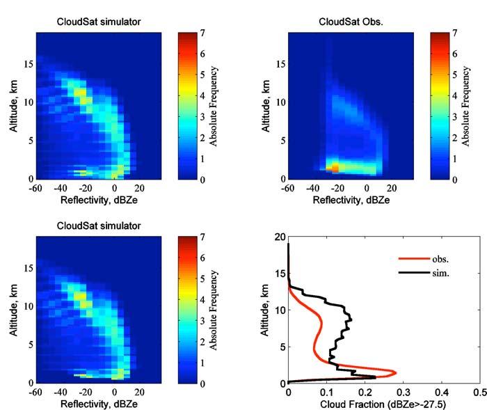
14 Marchand et al. 2008, Comparison of MMF with CloudSat Accepted JGR 05/2008 p. 14 In MAM the convergence zones over South America and Africa move northward (relative to DJF) and show lower fractional coverage than in DJF. Like the fall transition, this is reasonably well captured by the model. However by May, the model once again shows excessive hydrometeors in both the upper (7 to 20 km) and middle (3 to 7 km) troposphere over India, South East Asia, the western most tropical Pacific and the eastern tropical Pacific, as was noted earlier in the JJA data. (b) Histograms of Radar Reflectivity with Height We can gain further insight into the vertical distribution of hydrometeors by examining histograms of radar reflectivity with height. Figure 5 shows the model simulated (panels a, e) and CloudSat-observed (panels b, f) joint histogram of radar reflectivity with height above mean sea level for July and January in the tropical warm pool region (defined here as the region between 5 o S and 20 o N and between 70 o E to 150 o E following Webb at al., 2001). The model output for July (panel a) displays a characteristic curve with several modes, which are identified by red circles and which we will discuss momentarily. Here the height bins are spaced every 240 m (and simulated with 480 m resolution to emulate CloudSat observations) and reflectivity bins are 5 dbze wide. Model layers sometimes span more than 240 m or otherwise cross radar-resolution bin boundaries, which generates some discretization effects. CloudSat data display a similar structure but with almost no detections having a reflectivity less than about -30 dbze (due to the sensitivity limit of the radar). The presence of model hydrometeors with reflectivities below -30 dbze highlights the value of the radar simulator approach

15 Marchand et al. 2008, Comparison of MMF with CloudSat Accepted JGR 05/2008 p. 15 and the importance of using a reflectivity cut-off threshold when comparing model output with CloudSat observations in figures 1-4. The CloudSat observations in panel (b) also show no hydrometeor detections in a wedge near the surface (rising from the surface to about 1 km for reflectivities near -30 dbze). The wedge of missing-detections near the surface is a consequence of clutter in the radar measurements (Marchand et al. 2007). We can reproduce the effect of the surface clutter on cloud detections in the simulator output, as shown in panels (c) and (g), where detections near the surface have been removed. Panel (d) shows the profile of hydrometeor fraction for this region, where the simulated radar output from panel (c) and a dbze cut-off is used to derive the fractional coverage profile. Cloud detections near the surface were also removed in figures 1 and 4, to make comparison as objective as possible. Panel (d) shows that there is a large overestimate in hydrometeor fraction by the model at all altitudes for this region, as inferred earlier from Figures 2 through 4. Each mode identified in Figure 5 is dominated by a particular hydrometeor type. There is a low-altitude, low-reflectivity mode labeled 1 (located below 2 km and with reflectivities between roughly -40 and -20 dbze). This mode is associated with nondrizzling boundary layer clouds. We know this both because of our experience with cloud radar but also because we can turn on and off hydrometeor types in the radar simulation to see what effect they have on the resulting histograms. Because of surface clutter, CloudSat can not detect much of the non-drizzling boundary cloud predicted by the model.

16 Marchand et al. 2008, Comparison of MMF with CloudSat Accepted JGR 05/2008 p. 16 The model reflectivity-altitude histogram (panel a) shows a second mode in the altitude range between 0 and 5 km and with reflectivities above about -15 dbze. The radar reflectivity of hydrometeors in this mode is dominated by drizzle and rain. This does not mean that non-precipitating (cloud) water was not present at the same time and place as the rain or drizzle is observed; we can not determine this from reflectivity observations alone. Comparison of the model output with observations in this mode shows the model producing too much rain and drizzle. Those familiar with millimeter wavelength cloud-radar or longer wavelength radar systems maybe surprised to see reflectivity values for rain that are less than 20 dbze. The seemingly low reflectivity is the result of several factors. First, radars operating at 94 GHz (such as CloudSat) have a wavelength of about 3 millimeters. Rain and snow frequently have particle sizes comparable to or larger than this wavelength with the result that these particles do not Rayleigh scatter, but exhibit Mie-like resonances. Thus even heavy rain rates do not often generate reflectivity values much above 20 dbze at 94 GHz. Second, attenuation due to hydrometeors is higher at 94 GHz than for lower frequency radars. Attenuation rates as high as 10 db/km are not rare and CloudSat must generally penetrate thick overlying cloud structure to observe rainfall. Third, attenuation by water vapor is also higher at 94 GHz than at lower frequencies. A total attenuation due to water vapor from the top of atmosphere to the surface of 5 dbze is common in the moist tropics. Above 5 km, the model reflectivity-height histogram (figure 5, panel a) shows two additional modes. In the altitude range between about 5 and 10 km (mode 3), the reflectivity is dominated by precipitating ice and the fourth mode (primarily above 10

17 Marchand et al. 2008, Comparison of MMF with CloudSat Accepted JGR 05/2008 p. 17 km) is predominantly non-precipitating ice. Much of the non-precipitating ice predicted by the model is below the CloudSat sensitivity, particularly condensate above 15 km. Fortunately much of this condensate can be detected by lidar, such as the one on-board the NASA Calipso satellite (Winker et al. 2007). Comparison of Calipso and CloudSat observations does indeed show that there is a large amount of condensate at these altitudes that is not detected by CloudSat (Marchand et al. 2007). In future studies, we plan to apply a lidar simulator to the MMF output to further evaluate the model data. Nonetheless, restricting our comparison to the non-precipitating cloud that CloudSat can observe, we see the MMF is producing too much non-precipitating cloud. Figure 5, panels (e) and (f) show a similar comparison as panels (a) and (b), except for data averaged over January. The most noteworthy changes between the January and July CloudSat observations are a decrease in the amount of precipitating and nonprecipitating ice, a decrease in the amount of rain, and a slight increase in the amount of non-precipitating boundary layer cloud, such that in January the peak in high-level hydrometeor cover is comparable to the peak at low-levels; whereas in July the high-level coverage is much larger than the low-level hydrometeor coverage. While the total and relative amounts of observed precipitating and non precipitating hydrometeors differ in January from July, both months (actually all months throughout the year in this region) show a similar characteristic arc. (We note that while the shape of the arc is similar, the geographic location of most of the TWP hydrometeors has shifted southward over Indonesia, Figure 2). In Figure 5, the model does show a reduction in the amount of precipitating and non-precipitating ice and a decrease in the amount of rain, but also continues to have too many of these hydrometeors relative to the observations. The

18 Marchand et al. 2008, Comparison of MMF with CloudSat Accepted JGR 05/2008 p. 18 model also shows a marked increase in the amount and altitude of non-precipitating boundary layer clouds, which appear too abundant compared to the January CloudSat data. (c) Subtropics Overall, the model does a good job of reproducing the subtropical belts and their annual shift in position with respect to the mid-latitude storm tracks (Figure 1). The CloudSat observations and MMF model output both show the subtropics in the winter hemisphere having less high cloud than the subtropics in the summer hemisphere and a relative balance between the two hemispheres in the transition seasons. Perhaps the most noteworthy model shortcoming is the lack of hydrometeor fraction in the 1.2 to 3 km altitude range (Figure 4). This is true over both continental and oceanic regions and is particularly striking off the west coast of North America, South America, and southern Africa. The tendency of the model to produce too little low cloud cover (and too little precipitation) was found by Ovtchinnikov et al. (2006) for U.S. Southern Great Plains in a comparison against ground-based cloud radar observations, and more generally throughout the subtropics by Marchand et al. (2005) and Khiaroutdinov (2005) using observations from the International Cloud Climatology Project (ISCCP) and top of atmosphere fluxes (from the NASA CERES and ERBE missions). We examine the situation more closely in Figures 6 and 7, for the California stratus and Hawaiian trade cumulus zones, respectively. Following Webb et al. (2001), we define the California stratus zone as the region from 15 o to 35 o N and 110 o to 140 o W, and the Hawaiian trade cumulus zone as 15 o to 35 o N and 140 o W to 160 o E.

19 Marchand et al. 2008, Comparison of MMF with CloudSat Accepted JGR 05/2008 p. 19 Figure 6 (panel a) shows that in July, the model produces primarily non-precipitating clouds very close to the surface in the California Stratus zone. The model clouds are mostly too low for CloudSat to be able to detect (as shown in panel c), and indeed the CloudSat observations (panel b) show few low clouds. However, some fraction of the boundary layer clouds in this region are in fact high enough (or physically thick enough) for CloudSat to detect and we conclude that the model is producing clouds that are too close to the surface and not thick enough. Comparison of MMF output against ISCCP (Marchand et al. 2005) also found the MMF boundary layer clouds in this region to be to low, as have comparison of MMF cloud top heights against stereo-imaging retrievals by the NASA Multiangle Imaging Spectro-Radiometer (MISR, not shown). In January, the CloudSat observations (Figure 6) show a large increase in cloud above about 720 m (high enough for CloudSat to detect over ocean). While the model output shows that the boundary layer clouds have moved slightly higher relative to July, neither the amount nor height distribution matches the observations. In regard to high clouds, both CloudSat and the model show little high or mid-level cloud in July with a peak in occurrence above 10 km. However, the model shows virtually no hydrometeors between 2 and 5 km, whereas CloudSat detects some hydrometeors over this height interval. In January, both CloudSat and the model show a notable increase in the amount of high cloud with a peak below 10 km. The model shows more high cloud than is observed. In the Hawaiian trade cumulus zone, figure 7, the model non-precipitating boundary layer clouds are higher than in the California Stratus region, but they remain too low, particularly in January. In both July and January, the model shows more precipitation (hydrometeors with reflectivities greater than about -10 dbze) than the model, in and

20 Marchand et al. 2008, Comparison of MMF with CloudSat Accepted JGR 05/2008 p. 20 above the boundary layer. The model shows too much high cloud and precipitating ice in both seasons. This may well be related to the overly active Pacific ITCZ. The observations also indicate that the peak in radar detectable high cloud is above 10 km in July but below 10 km in January (figure 7 panel d), a trend that is at best weakly captured in the model. (d) Extratropics and Polar regions The position of the mid-latitude storm tracks and their relative strengths between the winter and summer hemisphere are well captured by the model as shown in Figure 1 (the zonally averaged hydrometeor fractional coverage with height), as well as in the broad regional distributions shown in Figures 3 and 4. Perhaps the most striking difference between the model output and observations in the extratropics and polar regions is a tendency for the model to overpredict the amount of low-level hydrometeor coverage. This is particularly noticeable in the northern hemisphere during JJA (Figure 1), because the model also underpredicts the amount of mid and high-level hydrometeor coverage poleward of 65 o N during this period. (On average the model very slightly overpredicts the mid-level and high-level hydrometeor coverage between about latitudes 50 o and 65 o during DJF). A similar pattern also occurs in the southern hemisphere during summer in that hemisphere (see DJF). The overestimate in northern hemisphere low-level JJA hydrometeors is wide spread with peaks in the northern hemisphere occurring over the North Pacific, Alaska and costal British Columbia, Newfoundland and the Labrador Sea, Baffin Island and Northern Hudson Bay, the North Atlantic, Greenland Sea, the Norwegian Sea and

21 Marchand et al. 2008, Comparison of MMF with CloudSat Accepted JGR 05/2008 p. 21 Norway, as well as parts of Russia, most notably Eastern Siberia. Most of these areas are observed to have large hydrometeor fractions, but not as high as found in the model. For the North Pacific, defined here as the region between 30 o to 60 o N and 160 o E to 140 o W following Norris and Weaver (2001), Figure 8 shows that in July the model generates too much hydrometeor coverage throughout the atmospheric column compared to the CloudSat observations. In particular, the model is producing large fractional coverage near the surface, with reflectivities near 0 dbze indicative of widespread lowlevel rain and drizzle. While much of this rain and drizzle would be too close to the surface for CloudSat to detect, the portion above about 720 m would be detected. The CloudSat observations (panel b) show relatively few hydrometeors between 720 m and 3 km, and what is detected has generally lower radar reflectivities indicative of clouds that do not contain significant drizzle. The presence of precipitating hydrometeors and an apparent lack of low-reflectivity clouds above 720 m is a common model feature of all the northern hemisphere areas listed above, where the model is observed to overpredict low-level hydrometeor coverage. Somewhat surprisingly, a comparison of MMF mean surface precipitation rates with estimates from the Global Precipitation Climatology Project (GPCP) (not shown) does not indicate that the model significantly overpredicts surface precipitation in the North Pacific (or zonally averaged in either mid-latitude storm track for that matter). This suggests that the MMF likely has too little heavy precipitation and too much drizzle and light precipitation in this region. The zonally averaged hydrometeor coverage at mid and high levels is slightly too large in the model for latitudes between 50 o and 65 o in the northern hemisphere summer (Figure 1). Much of this overprediction occurs over the North Pacific, southern Alaska

22 Marchand et al. 2008, Comparison of MMF with CloudSat Accepted JGR 05/2008 p. 22 and coastal British Columbia. Outside of the North Pacific, the total model hydrometer coverage at mid and high levels more nearly matches the observations. In September, the model hydrometeor coverage increases significantly throughout the arctic and northern hemisphere extratropics, especially above 3 km in the artic (not shown). For the most part, profiles of total hydrometeor coverage in the model compare favorably with CloudSat observations from September through April with the model tending to slightly overestimate the hydrometeor fraction, as exemplified in Figure 8 for January over the North Pacific. In the North Pacific the CloudSat observations for January show a large increase in both precipitating hydrometeors and in low-reflectivity water clouds compared to July. The profile of hydrometeor fraction between the model and observations (shown in panel h) are in fair agreement at low levels, despite the fact that the observations show much more low-reflectivity boundary layer clouds than the model. Interestingly above 3 km, the CloudSat observations in January seem to show two distinct ice modes (or characteristic curves), one mode where -25 dbze reflectivities peak near 10 km and one mode where -25 dbze reflectivities peak between 6 and 7 km. It is not clear whether these modes are real or an artifact of the limited CloudSat swath and sampling. However, we observe that the CloudSat data for December (not shown) display a single ice mode similar to the upper branch in the January data and the data for February (not shown) display a single ice mode similar to the lower branch. Poleward of about 65 o north latitude, the model dramatically underestimates the mid and high-level hydrometeor coverage during the northern hemisphere summer. CloudSat carries a near-nadir looking radar that does not scan and flies in a fixed sun-synchronous orbit and so does not collect data much closer than about 9 o to either the North or South

23 Marchand et al. 2008, Comparison of MMF with CloudSat Accepted JGR 05/2008 p. 23 Pole. However, latitudes between 65 o and 80 o are heavily sampled and the radar observations are equally good during polar day or night conditions. In Figure 9, we examine the situation in more detail over the Beaufort Sea (defined here as region between 70 o to 80 o N and 125 o to 170 o W). As found in the North Pacific during July, the model generates wide spread precipitating hydrometeors near the surface, most of which is too close to the surface for CloudSat to observe and that portion which could be observed does not match the observations which show less total coverage and lower reflectivities. However in marked contrast to the North Pacific, the model substantially underestimates the total hydrometeor coverage above about 1.5 km. While we highlight the Beaufort Sea, here, this same pattern is found throughout much of the arctic in JJA. During DJF, the model total hydrometeor coverage over much of the arctic compares favorably with the observations, as is the case for the North Pacific (and midlatitudes, generally). One region where this is not the case is over the Beaufort Sea (as well as nearby Queen Ann Islands, not shown). Figure 9 shows that in January, the model overestimates the hydrometeor coverage below 5 km in the Beaufort Sea. While the model does predict substantially more low-reflectivity boundary layer cloud, this cloud is very close to the surface and doesn t appreciably add to the total coverage profiles shown in panel h, because it would not be detected by CloudSat due to surface clutter limitations of the radar. Above 5 km, the model total hydrometeor coverage (above the dbze threshold) compares favorably with the observations. However, we note that in the Artic much of the model predicted hydrometeors have reflectivities below the dbze threshold. The low reflectivities are a result of cold atmospheric temperatures and limited water vapor generally producing small amounts of condensed ice, which in turn

24 Marchand et al. 2008, Comparison of MMF with CloudSat Accepted JGR 05/2008 p. 24 result in small effective radii in the model bulk microphysical scheme. Low condensate amounts and small particle sizes both lead to small radar reflectivities. As such, the total hydrometeor coverage comparison may prove to be quite sensitive to the model microphysical treatment. A similar effect is observed over the Antarctic (not shown). In the southern hemisphere over the southern oceans, the model total hydrometeor coverage profiles generally compare very favorably with CloudSat observations, as exemplified by the South Pacific, shown in figure 10. The model tends to overestimate the peak in low-level hydrometeors during the southern hemisphere summer (as shown for January). As in the northern hemisphere extratropics, the boundary layer reflectivites tend to be too high and the distribution of reflectivties at all altitudes tends to be narrow. In the winter months (May September), there is too much precipitating condensate at all altitudes much as is the case for the North Pacific during the northern hemisphere winter. 5. Conclusions and Future Work In this article we compare output from a Multiscale Modeling Framework Global Climate Model with radar observations from the NASA CloudSat mission using a radar simulator approach. Overall we found that the MMF model does a good job of reproducing the broad pattern of tropical convergence zones, subtropical belts, and midlatitude storm tracks, as well as, their changes in position with the annual solar cycle. Nonetheless, the comparison also reveals a number of model shortfalls including: (1) Excessive hydrometeor coverage throughout the Asian Monsoon region at all altitudes from May through November. These large fractions are associated

25 Marchand et al. 2008, Comparison of MMF with CloudSat Accepted JGR 05/2008 p. 25 with excessive cloud radiative forcing (Marchand et al. 2005) and surface precipitation (Khairoutdinov et al 2005). The monsoon appears to set up too soon (May), dissipates to late (November), and reaches a peak in August, whereas the observations show peak coverage (fractions) in June or July. (2) Excessive hydrometeor coverage at all altitudes over Indonesia and in the South Pacific Convergence Zone (SPCZ) from December through March. (3) Excessive hydrometeor coverage along the ITCZ in the central and eastern Pacific during the northern hemisphere summer. This is particularly strong at low and mid levels. (4) A thin band of low-level hydrometeors in the southern hemisphere of the central (and at times eastern and western) Pacific that is not observed by CloudSat. In some ways this band resembles a second much weaker ITCZ, however hydrometeors in this band are largely restricted to low altitudes. It occurs throughout the annual cycle but is most distinct in February through April. (5) A lack of hydrometeors in the 1.2 to 3 km altitude range over all subtropical oceanic basins. This is particularly striking off the west coast of North America, South America, and southern Africa regions well known for extensive stratocumulus. The low clouds that are predicted by the model in these regions are too low (or too shallow) and often extend into the lowest model layers. (6) Excessive low-level hydrometeor coverage in the mid-latitude storm tracks of both hemispheres during the summer season (JJA in the northern hemisphere,

26 Marchand et al. 2008, Comparison of MMF with CloudSat Accepted JGR 05/2008 p. 26 DJF in the sourthern hemisphere). These hydrometeors have reflectivities dominated by the presence of precipitating liquid water, such that the distribution of reflectivity in the model is disproportionately weighted toward larger values as compared to the CloudSat observations. (7) Excessive hydrometeor coverage at all altitudes in the North Pacific and the Southern Oceans during the winter season in each hemisphere. (8) Poleward of 65 o latitude, the model generally underestimates the mid and high level hydrometeor coverage during the summer season in each hemisphere and overestimates low-level hydrometeors (except over the Antarctic highlands) throughout the year. The overprediction of hydrometeor coverage around the Asian Monson region (and other tropical convergences zones more generally) during JJA and over the SPCZ and southern oceans during January was identified by Khairoutdinov et al. (2001, 2005) and Marchand et al. (2005) largely based on examination of surface precipitation and top of atmosphere fluxes. The CloudSat observations clearly confirm these conclusions, as well as add additional details on the vertical structure that can be used to quantitatively gauge improvements in future versions of the MMF. Likewise the model underestimate of low clouds in the subtropics, identified here was also identified by Khairoutdinov et al. (2005) and Marchand et al (2005) based largely on comparisons against ISCCP data at least for those regions dominated by stratocumulus. While surface clutter clearly limits CloudSat to detecting clouds more than about 720 m above the surface, CloudSat should still prove useful for some boundary layer cloud studies. Some of the other model

27 Marchand et al. 2008, Comparison of MMF with CloudSat Accepted JGR 05/2008 p. 27 deficiencies identified in this study, such as the excessive low-level hydrometeor coverage in the mid-latitude storm tracks and in polar regions at various times of the year, are largely possible because of the radar s ability to penetrated clouds and to work equally well during day or night. Joint histograms of reflectivity and height show that regions tend to have a characteristic curve with several modes associated with precipitating and nonprecipitating ice and liquid water. The shape of the curve varies from region to region. In most regions the model often reproduces the overall shape reasonably well, but not necessarily the intensity (fractional coverage) of the hydrometeor types. Also, the observed distribution of reflectivity at any given altitude tends to be broader than the model predicted distribution. This effect appears common in many regions, but is most noticeable during the winter months at mid and high latitudes (see Figures 8 through 10). We believe that the model distribution is too narrow primarily because of the simple nature of the model bulk microphysical scheme. The analysis involved monthly and seasonal averages using 4 years of model output. The model runs use observed sea surface temperatures from 1998 through 2002, while one year of CloudSat observations are used, starting from June The variations in the model output from year to year are small relative to the difference between the model and CloudSat observations discussed here. Nonetheless, we recognize that (weak) El Nino conditions were in place during winter of 2007 whereas the model simulations occur during La Nina years. In the future we plan to conduct model runs using sea surface temperatures from 2006 and We also note that the MMF data were not subsampled to reproduce the orbital characteristic of CloudSat, but rather includes

28 Marchand et al. 2008, Comparison of MMF with CloudSat Accepted JGR 05/2008 p. 28 observations from all times of day. In the future we also plan to output model data to support such sub-sampling, and to study quantitatively the effect such sampling may introduce in the monthly and seasonal means. Here we examine zonally averaged profiles of hydrometeor fractional coverage, the global geographic distribution in three altitude ranges and histograms of radar reflectivity with height for a few select regions. CloudSat provides much more information on the structure of cloud fields then revealed by these quantities. For example, the twodimensional transects observed by CloudSat also provide information on cloud base distributions and vertical cloud overlap, as well as vertical and horizontal covariances in cloud occurrence and reflectivity. These later quantities are somewhat sensitive to the horizontal and vertical scales used when calculating them, and we are currently researching how to use them for model evaluation. Nonetheless, even the simple observables used in this study enable us to identify a variety of model deficiencies and can clearly be used to gauge potential improvements in future versions of the MMF. It should also be mentioned that while this study compares monthly averages, these observables can be aggregated in many ways to potentially yield additional insights into how to improve the model; for example analyzing model performance as a function of the atmosphere thermodynamic state. In the future, we plan to undertake one such analysis following the approach discussed by Marchand et al (2006). The comparisons of model output with CloudSat observations in Figures 1 through 4 use a common radar reflectivity threshold of dbze. Such is necessary because the model sometimes contains hydrometeors whose reflectivity is well below the CloudSat radar sensitivity, and so one can t simply compare CloudSat observed profiles with

29 Marchand et al. 2008, Comparison of MMF with CloudSat Accepted JGR 05/2008 p. 29 profiles of all model hydrometeors. We choose dbze rather than -30 dbze to minimized the effect of false positives, which becoming increasing common as one nears radar sensitivity limit. In some situations, most notably in the upper troposphere and in polar regions, the model contains large amounts of hydrometeors with reflectivities below the dbze threshold, such that the resulting profiles of hydrometeor coverage are likely sensitive to the details of the model microphysical formulation and the reflectivity threshold. It would take a significantly more sensitive radar (~ -40 dbze) to detect the bulk of these low-reflectivity hydrometeors. Fortunately, in the near future CloudSat observations will be combined with observations from the CALIPSO lidar to retrieve estimates of the particle size and condensate amount (where both sensors are able to detect clouds). In many circumstances, this will enable use to gauge to what degree differences in model and observed hydrometeor profiles are due to differences in condensate amount and what is due to the particle size. The comparisons presented here demonstrate the diagnostic utility of CloudSat in combination with a radar simulator approach. The radar simulator can be used to estimate the reflectivity from lower frequencies radars such 14 GHz system used by the NASA Tropical Rainfall Measurement Mission (TRMM) and comparison of MMF output against TRMM observations is ongoing (Zhang et al. 2008). Finally we note that the radar simulator used here takes advantage of the high-resolution data produced by the MMF, but with appropriate cloud and precipitation overlap models the radar simulator could be applied to traditional climate models, as well.

30 Marchand et al. 2008, Comparison of MMF with CloudSat Accepted JGR 05/2008 p. 30 Acknowledgements The authors would like to express their thanks to Phil Partain, Don Reinke and the entire staff of the CloudSat Data Processing Center at CIRA/Colorado State University for gathering, processing and providing CloudSat data. Thanks also to Steve Durden, Simone Tanelli and all those at NASA Jet Propulsion Laboratory for their efforts in developing CloudSat and calibrating the radar measurements. Finally, we would like to express our thanks to the Department of Energy and Pacific Northwest National Laboratory for their support and, in particular, for providing time on the MPP2 supercomputer needed to run the MMF climate model.

31 Marchand et al. 2008, Comparison of MMF with CloudSat Accepted JGR 05/2008 p. 31 References Battaglia, A., M. O. Ajewole and C. Simmer, 2007: Evaluation of radar multiple scattering effects in Cloudsat configuration, Atmos. Chem. Phys. 7,7, Battaglia, A., and C. Simmer, 2008: How does multiple scattering affect the spaceborne W-band radar measurements at ranges close to and crossing the surface-range?, IEEE Transactions on Geoscience and Remote Sensing, 46 (6), Boville, B.A., P. J. Rasch, J. J. Hack, AND J. R. McCAA, 2006: Representation of Clouds and Precipitation Processes in the Community Atmosphere Model Version 3 (CAM3), J. Climate, vol. 19 p Collins, W. D., P. J. Rasch, B. A. Boville, J. J. Hack, J. R. McCaa, D. L. Williamson, B. P. Briegleb, C. M. Bitz, S-J. Lin, and M. Zhang, 2006: The formulation and atmospheric simulation of the Community Atmosphere Model Version 3 (CAM3). J. Climate, 19(11), Collins, W. D., P. J. Rasch, B. A. Boville, J. J. Hack, J. R. McCaa, D. L. Williamson, J. T. Kiehl, B. Briegleb, C. Bitz, *S.-J. Lin, M. Zhang, and Y. Dai, 2004: Description of the NCAR Community Atmosphere Model (CAM 3.0). NCAR Tech. Note NCAR/TN- 464+STR, 226 pp. Demott, C.A., D. A. Randal, M. Khairoutdinov, 2007: Convective Precipitation Variability as a Tool for General Circulation Model Analysis, Journal of Climate, 20, Grabowski, W. W., Coupling cloud processes with the large-scale dynamics using the cloud-resolving convection parameterization (CRCP), J. Atmos. Sci., 68, , Haynes J. M., R. T. Marchand, Z. Luo, A. Bodas-Salcedo, and G. L. Stephens, 2007 A Multipurpose Radar Simulation Package: QuickBeam. Bulletin of the American Meteorological Society, Vol. 88, Issue 11 (November 2007) pp DOI: /BAMS Khairoutdinov, M. F., and D. A. Randall, A cloud resolving model as a cloud parameterization in the NCAR Community Climate Model: Preliminary results, Geophys. Res. Letters, 28, , Khairoutdinov, M. F., and D. A. Randall, Cloud resolving modeling of the ARM Summer 1997 IOP: Model formulation, results, uncertainties, and sensitivities, J. Atmos. Sci., 60, , Khairoutdinov, M. F., D. A. Randall, and C. DeMott, Simulations of the atmospheric general circulation using a cloud-resolving model as a super-parameterization of physical processes, J. Atmos. Sci., 62, , 2005.

32 Marchand et al. 2008, Comparison of MMF with CloudSat Accepted JGR 05/2008 p. 32 Kristjansson, J. E., J. M. Edwards, and D. L. Mitchell, 2000: Impact of a new scheme for optical properties of ice crystals on climates of two GCMs. J. Geophys. Res., 105, Lemke, M. H., and M. Quante (1999), Backscatter characteristics of nonspherical ice crystals: Assessing the potential of polarimetric radar measurements, J. Geophys. Res., 104(D24), 31,739 31,752. Liebe, H.J., An updated model for millimeter wave propagation in moist air, Radio Sci., 20, , Marchand, R., G.G. Mace, T. Ackerman, and G. Stephens, 2008: Hydrometeor Detection Using Cloudsat An Earth-Orbiting 94-GHz Cloud Radar. J. Atmos. Oceanic Technol., 25, Marchand, R.T., N. Beagley, S. Thompson, T.P. Ackerman, D. M. Schultz, 2006 A Bootstrap Technique for Testing the Relationship Between Local-Scale Radar Observations of Cloud Occurrence and Large-Scale Atmospheric Fields, Journal of the Atmospheric Sciences, Vol. 63, No. 11, pages Marchand, R. T., S. J. Ghan, M. Ovtchinnikov, T. P. Ackerman, and M. Khairoutdinov, 2005 Comparison of the Multi-scale Modeling Framework and NCAR Community Atmospheric Model (CAM) with ISCCP and CERES Retrievals, 16th Conference on Climate Variability and Change, AMS Annual Meeting, San Deigo, Jan McFarlane, S. A., J. H. Mather, and T. P. Ackerman, 2007: Analysis of tropical radiative heating profiles: A comparison of models and observations, J. Geophys. Res., 112, D14218, doi: /2006jd Norris, J. and C. Weaver, 2001 Improved techniques for evaluating GCM cloudiness applied to the NCAR CCM3, J. of Climate, 14, Ovtchinnikov, Mikhail, Thomas P. Ackerman, Roger T. Marchand, and Marat Khairoutdinov, 2005 Evaluation of the Multi-Scale Modeling Framework Using Data from the Atmospheric Radiation Measurement Program, Journal of Climate, 19 (9): MAY Randall, D., M. Khairoutdinov, A. Arakawa, and W. Grabowski, 2003: Breaking the cloud parameterizations deadlock, Bull. Amer. Meteor. Soc., 84, Sato, K., and H. Okamoto, 2006: Characterization of Ze and LDR of nonspherical and inhomogeneous ice particles for 95-GHz cloud radar: Its implication to microphysical retrievals, J. Geophys. Res., 111, D22213, doi: /2005jd

33 Marchand et al. 2008, Comparison of MMF with CloudSat Accepted JGR 05/2008 p. 33 Stephens, Graeme L., Deborah G. Vane, Ronald J. Boain, Gerald G. Mace, Kenneth Sassen, Zhien Wang, Anthony J. Illingworth, Ewan J. O'Connor, William B. Rossow, Stephen L. Durden, Steven D. Miller, Richard T. Austin, Angela Benedetti, Cristian Mitrescu, and CloudSat Science Team, 2002: The CloudSat mission and the A-train: A new dimension of space-based observations of clouds and precipitation. Bull. Amer. Meteorol. Soc., 83, , doi: /bams Tanelli, Simone, Stephen L. Durden, Eastwood Im, Kyung S. Pak, Dale G. Reinke, Philip Partain, John M. Haynes, and Roger T. Marchand, 2008: CloudSat s Cloud Profiling Radar after 2 years in orbit: performance, calibration, and processing, IEEE trans. Geosci. Rem. Sens., accepted. Webb, M., C. Senior, S. Bony, J. J. Morcrette, 2001: Combining ERBE and ISCCP data to assess clouds in the Hadley Center, ECMWF and LMD atmospheric climate models, Climate Dynamics, 17, Winker, D. M., B. H. Hunt, and M. J. McGill, 2007: Initial performance assessment of CALIOP, Geophys. Res. Lett., 34, L19803, doi: /2007gl Zhang, Y., S. A. Klein, C. Liu, B. Tian, R. T. Marchand, J. M. Haynes, R. B. McCoy, Y. Zhang, and T. P. Ackerman (2008), On the diurnal cycle of deep convection, high-level cloud, and upper troposphere water vapor in the Multiscale Modeling Framework, J. Geophys. Res., 113, D16105, doi: /2008jd009905

34 Marchand et al. 2008, Comparison of MMF with CloudSat Accepted JGR 05/2008 p. 34 List of Figures Figure 1 Intensity plots of monthly zonal profiles of radar hydrometeor fraction (dbze>-27.5). (left column) CloudSat observations (right column) model simulated radar output. Vertical axis is height above mean sea level (in km) and horizontal axis is latitude. CloudSat is a near-nadir pointing instrument and so does not obtain full pole-topole coverage. The radar also suffers from ground-clutter effects and is unable to detect most cloud with in 1.2 km of the surface (Marchand et al. 2007). Missing detections near the surface due to surface clutter are accounted for in the radar simulation process. Figure 2 Intensity plots of June through March monthly peak radar hydrometeor fraction between 7 and 20 km above mean sea level (dbze>-27.5). (left column) CloudSat observations (right column) model simulated radar cloud fraction. Figure 3 As figure 2, except for 3 to 7 km above mean sea level. Figure 4 As figure 2, except for 1.2 to 3 km above mean sea level. Figure 5 Joint histograms radar reflectivity and height for the Tropical Warm Pool (defined here as the region between 40 o S and 20 o N and between 70 o E to 150 o E following Webb at al. 2001). Top panels (a-d) are for July and bottom panels (e-f) for January. Red circles indicate hydrometeor modes discussed in the text. Panels (a, c, and e) are radar simulation using MMF output and Right panels (b and f) are CloudSat observations. Panel (c) is the same as panel (a) except missing detection because of ground clutter and considered. Panel (d) shows mean occurrence profiles for observations and simulation (including the effect of lost detections due to surface clutter). Figure 6 As figure 5, except for the California Stratus region (15 o to 35 o N and 110 o to 140 o W). Figure 7 As figure 5, except for the Hawaiian trade cumulus region (15 o to 35 o N and 140 o W to 160 o E). Figure 8 As figure 5, except for the North Pacific (30 o to 60 o N and 160 o E to 140 o W). Figure 9 As figure 5, except for Beaufort Sea (70 o to 80 o N and 125 o E to 170 o W). Figure 10 As figure 5, except for the South Pacific (30 o to 60 o S and 80 o to 180 o W).

35

36

37

38

39

40

41