Methods of Computer Simulation. Molecular Dynamics and Monte Carlo

Size: px

Start display at page:

Download "Methods of Computer Simulation. Molecular Dynamics and Monte Carlo"

Gary Mosley
5 years ago
Views:

1 Molecular Dynamics Time is of the essence in biological processes therefore how do we understand time-dependent processes at the molecular level? How do we do this experimentally? How do we do this computationally? 1

2 Methods of Computer Simulation Molecular Dynamics and Monte Carlo 2

3 3

4 What Is Molecular Dynamics? Simulating the Brownian motion of proteins (and other macromolecules). Formally, solving Newton s equations of motion for every atom in the system. Connecting the trajectory with thermodynamic properties. Ultimately, understanding macromolecular properties from first principles. What is a molecular dynamics simulation? Simulation that shows how the atoms in the system move with time Typically on the nanosecond timescale Atoms are treated like hard balls, and their motions are described by Newton s laws. 4

5 5

Characteristic protein motions Type of motion Timescale Amplitude Local: bond stretching angle bending methyl rotation Medium scale loop motions SSE formation 0.01 ps 0.

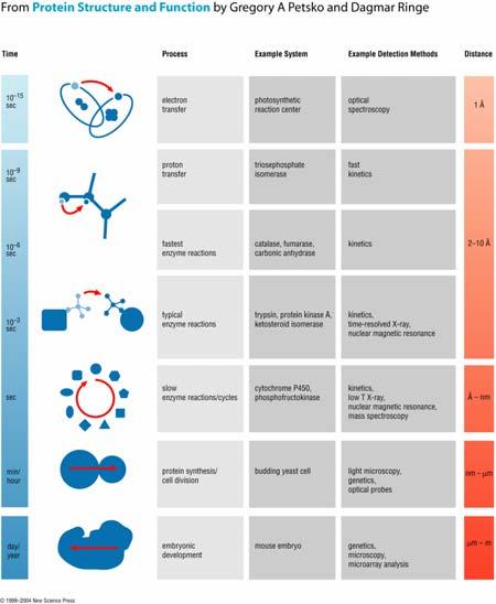
6 Characteristic protein motions Type of motion Timescale Amplitude Local: bond stretching angle bending methyl rotation Medium scale loop motions SSE formation 0.01 ps 0.1 ps 1 ps ns µs < 1 Å 1-5 Å Periodic (harmonic) Global protein tumbling (water tumbling) protein folding 20 ns (20 ps) ms hrs > 5 Å Random (stochastic) Energy Landscape 1 ms to 1s Barrier crossing time ~ exp[barrier Height] 1 µs Barrier Height Unfolded State Expanded, disordered Molten Globule Compact, disordered Native State Compact, Ordered 6

7 Why MD simulations? Link physics, chemistry and biology Model phenomena that cannot be observed experimentally Understand protein folding Access to thermodynamics quantities (free energies, binding energies, ) 7

8 Why do we do computer simulations in biophysics and biochemistry? Systems with many particles behave in qualitatively different ways than systems with a small number of particles By simulating a system in thermal equilibrium, we can see qualitativelyand quantitatively what is happening. We can calculate explicit observable quantities to confirm that our model (and our understanding of the system) is correct. If we succeed, we will be able to predict behavior that we would not expect without the simulations. The goal of computation is understanding not numbers. 8

9 How do you run a MD simulation? Get the initial configuration From x-ray crystallography or NMR spectroscopy (PDB) Assign initial velocities At thermal equilibrium, the expected value of the kinetic energy of the system at temperature T is: N Ekin = m v 2 i i = (3N ) kbt 2 i= 1 2 This can be obtained by assigning the velocity components vi from a random Gaussian distribution with mean 0 and standard deviation (k B T/m i ): v = 2 i kbt m i How do you run a MD simulation? For each time step: Compute the force on each atom: E F( X ) = E( X ) = X Solve Newton s 2 nd law of motion for each atom, to get new coordinates and velocities M X = Store coordinates F(X ) X: cartesian vector of the system M diagonal mass matrix.. means second order differentiation with respect to time Stop Newton s equation cannot be solved analytically: Use stepwise numerical integration 9

10 What the integration algorithm does Advance the system by a small time step t during which forces are considered constant Recalculate forces and velocities Repeat the process If t is small enough, solution is a reasonable approximation 10

11 Molecular dynamics (MD) simulations A deterministic method based on the solution of Newton s equation of motion F i = m i a i for the ith particle; the acceleration at each step is calculated from the negative gradient of the overall potential, using F i = - grad E i -= - E i Newton s Laws r r F= ma 2r dr r r m = UE 2 ( ) dt r In general, is a 3Ndimensional vector 11

12 E i = Σ k (energies of interactions between i and all other residues k located within a cutoff distance of R c from i) E i = Gradient of potential? Derivative of E with respect to the position vector r i = (x i, y i, z i ) T at each step a xi ~ - E/ x i a yi ~ - E/ y i a zi ~ E/ z i Interaction potentials include; Non-Bonded Interaction Potentials Electrostatic interactions of the form E ik (es) = q i q k /r ik Van de Waals interactions E ij (vdw) = - a ik /r ik 6 + b ik /r ik 12 Bonded Interaction Potentials Bond stretching E i (bs) = (k bs /2) (l i l i0 ) 2 Bond angle distortion E i (bad) = (k θ /2) (θ i θ i0 ) 2 Bond torsional rotation E i (tor) = (k φ /2) f(cosφ i ) 12

13 A Potential Energy Function 1 1 V = Kb b b + K 2 2 bonds ( ) ( θ θ ) 1 + Kφ 1+ cos 2 dihedral angles θ 0 bond angles ( nφ δ) 1 A C qq nonbonded pairs r 6 r εr 13

14 14

15 Statistical Mechanics Ensemble very many copies of the system of interest evolving independently. Calculate averages of important quantities over the ensemble. Thermodynamic quantities can be derived from the appropriate averages. The Ergodic Hypothesis Averages taken over a single system for a sufficiently long time will yield the same values as ensemble averages. Molecular dynamics generates the values to be averaged. Practical issues: How long is long enough? Is the force field U(r) good enough? 15

16 16

17 17

18 Without the out-of-plane term, the bonded structures would behave differently To achieve the desired geometry (known from experiments) additional terms should be added in the force field (these help a benzene ring to be planar!) E(w)= k(1-cos2w) is one way... Cross-terms: 1, 2 and 3 force fields The presece of cross terms in a force field reflects couplings between the internal coordinates. As a bond angle is decreased, it is found that the adjacent bonds stretch to reduce the interaction between the 1,3 atoms. 18

19 Types of cross-terms Stretch-stretch Stretch-torsion Stretch-bend Bend-torsion Bend-bend 19

20 Example 1: gradient of vdw interaction with k, with respect to r i E ik (vdw) = - a ik /r ik 6 + b ik /r ik 12 r ik = r k r i x ik = x k x i y ik = y k y i z ik = z k z i r ik = [ (x k x i ) 2 + (y k y i ) 2 + (z k z i ) 2 ] 1/2 E/ x i = [- a ik /r ik 6 + b ik /r ik 12 ] / x i where r ik6 = [ (x k x i ) 2 + (y k y i ) 2 + (z k z i ) 2 ] 3 20

21 Example 2: gradient of bond stretching potential with respect to r i E i (bs) = (k bs /2) (l i l i0 ) 2 l i = r i+1 r i l ix = x i+1 x i l iy = y i+1 y i l iz = z i+1 z i l i = [ (x i+1 x i ) 2 + (y i+1 y i ) 2 + (z i+1 z i ) 2 ] 1/2 Ei(bs) = (k bs /2) (l i l i0 ) 2 E i (bs) / x i = - m i a ix (bs) (induced by deforming bond l i ) = (k bs /2) {[ (x i+1 x i ) 2 + (y i+1 y i ) 2 + (z i+1 z i ) 2 ] 1/2 l i0 } 2 / x i = k bs (l i l i0 ) {[ (x i+1 x i ) 2 + (y i+1 y i ) 2 + (z i+1 z i ) 2 ] 1/2 l i0 }/ x i = k bs (l i l i0 ) (1/2) (l i -1 ) (x i+1 x i ) 2 / x i = - k bs (1 l i0 / l i ) (x i+1 x i ) 21

22 The Verlet algorithm Perhaps the most widely used method of integrating the equations of motion is that initially adopted by Verlet [1967].The method is based on positions r(t), accelerations a (t), and the positions r(t -dt) from the previous step. The equation for advancing the positions reads as r(t+dt) = 2r(t)-r(t-dt)+ dt 2 a(t) There are several points to note about this equation. It will be seen that the velocities do not appear at all. They have been eliminated by addition of the equations obtained by Taylor expansion about r(t): You need r(t) and r(t-dt) r(t+dt) = r(t) + dt v(t) + (1/2) dt 2 a(t)+... to find r r(t+dt) r(t-dt) = r(t) - dt v(t) + (1/2) dt 2 a(t)- The velocities are not needed to compute the trajectories, but they are useful for estimating the kinetic energy (and hence the total energy). They may be obtained from the formula v(t)= [r(t+dt)-r(t-dt)]/2dt i F i Time=t+dt Time=t 22

23 Initial velocities (v i ) using the Boltzmann distribution at the given temperature v i = (m i /2πkT) 1/2 exp (- m i v i2 /2kT) How to generate MD trajectories? Known initial conformation, i.e. r i (0) for all atom i Assign v i (0), based on Boltzmann distribution at given T Calculate r i (δt) = r i (0) + δt v i (0) Using new r i (δt) evaluate the total potential V i on atom i Calculate negative gradient of V i to find a i (δt) = - V i /m i Start Verlet algorithm using r i (0), r i (δt) and a i (δt) Repeat for all atoms (including solvent, if any) Repeat the last three steps for ~ 10 6 successive times (MD steps) 23

24 A widely-used algorithm: Leap-frog Verlet Using accelerations of the current time step, compute the velocities at half-time step: v(t+ t/2) = v(t t/2) + a(t) t Then determine positions at the next time step: X(t+ t) = X(t) + v(t + t/2) t v X v t- t/2 t t+ t/2 t+ t t+3 t/2 t+2 t Choosing a time step t Not too short so that conformations are efficiently sampled Not too long to prevent wild fluctuations or system blow-up An order of magnitude less than the fastest motion is ideal Usually bond stretching is the fastest motion: C-H is ~10fs so use time step of 1fs Not interested in these motions? Constrain these bonds and double the time step 24

25 Minimization Energy minimization is very widely used in molecular modelling and is an integral part of techniques such as conformational search procedures. Min is also used to prepare a system for MD in order to relieve any unfavorable interactions in the initial configuration of the system. Especially important in complex systems such as proteins. Energy Minimization Local minima: A conformation X is a local minimum if there exists a domain D in the neighborhood of X such that for all Y X in D: U(X) <U(Y) Global minimum: A conformation X is a global minimum if U(X) <U(Y) for all conformations Y X 25

26 The minimizers Some definitions: Gradient: The gradient of a smooth function f with continuous first and second derivatives is defined as: Hessian f f f ( X ) =... f... x1 x The n x n symmetric matrix of second derivatives, H(x), is called the Hessian: 2 f 2 x f H ( x) = xi x f xn x f x1 x j... 2 f xi x j... 2 f x x N i x N j f x1 x... 2 f xi x... 2 f 2 x N N N The minimizers Minimization of a multi-variable function is usually an iterative process, in which updates of the state variable x are computed using the gradient, and in some (favorable) cases the Hessian. Iterations are stopped either when the maximum number of steps (user s input) is reached, or when the gradient norm is below a given threshold. Steepest descent (SD): The simplest iteration scheme consists of following the steepest descent direction: (α sets the minimum along the line defined xk+ 1 = xk α f ( xk ) by the gradient) Usually, SD methods leads to improvement quickly, but then exhibit slow progress toward a solution. They are commonly recommended for initial minimization iterations, when the starting function and gradient-norm values are very large. 26

27 Minimization Minimization follows gradient of potential to identify stable points on energy surface Let U(x) = a/2(x-x0)2 Begin at x, how do we find x0 if we don t know U(x) in detail? How can we move from x to x0? Steepest descent based algorithms (SD): x x = x+δ δ = -κ U(x)/ x = -κa(x- x 0) This moves us, depending on κ, toward the minimum. On a simple harmonic surface, we will reach the minimum, x0, i.e. converge, in a certain number of steps related to κ. SD methods use first derivatives only SD methods are useful for large systems with large forces Conjugate gradients (CG): The minimizers In each step of conjugate gradient methods, a search vector p k is defined by a recursive formula: pk + 1 = f ( xk ) + βk+ 1pk The corresponding new position is found by line minimization along p k : the CG methods differ in their definition of b: - Fletcher-Reeves: - Polak-Ribiere - Hestenes-Stiefel x k +1 β β β = x k + λ p k f ( xk+ 1) f ( xk 1) f ( x ) f ( x ) FR + k+ 1 = k k PR f ( xk + 1) f ( xk+ 1 k+ 1 = f ( xk ) f HS k+ 1 f ( xk+ 1 = p k k [ ) f ( x )] ( x ) ) [ f ( xk+ 1) f ( xk )] [ f ( x ) f ( x )] k + 1 k k k 27

28 Newton s methods: The minimizers Newton s method is a popular iterative method for finding the 0 of a one-dimensional function: x k+ 1 = xk g g ( xk ) '( x ) k It can be adapted to the minimization of a one dimensional function, in which case the iteration formula is: g' ( xk ) xk+ 1 = xk g' '( x ) The equivalent iterative scheme for multivariate functions is based on: x k+ 1 = x k H 1 k x 3 ( x ) f ( x ) k Several implementations of Newton s method exist, that avoid computing the full Hessian matrix: quasi-newton, truncated Newton, adopted-basis Newton-Raphson (ABNR), k k x 2 x 1 x 0 28

29 29

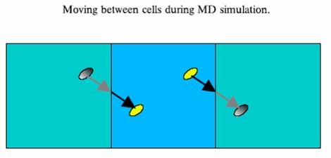
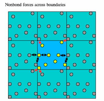
30 Periodic boundary conditions 30

31 31

32 32

33 33

34 34

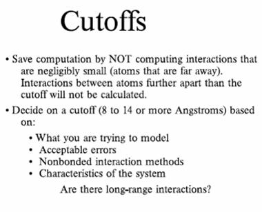
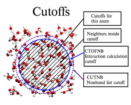
35 Notes on computing the energy Bonded interactions are local, and therefore their computation has a linear computational complexity (O(N), where N is the number of atoms in the molecule considered. The direct computation of the non bonded interactions involve all pairs of atoms and has a quadratic complexity (O(N2)). This is usually prohibitive for large molecules. U NB = 12 6 R ij Rij ε ij 2 + rij rij i, j nonbonded q q i, j nonbonded 0 i j 4πε εr ij Reducing the computing time: use of cutoff in U NB Notes on computing the energy Tamar Schlick, Molecular Modeling and Simulation, Springer 35

36 36 ( ) ( ) + = j i ij j i ij ij j i ij ij ij ij ij ij ij NB r q q r S r R r R r S U, 0, ε πε ω ε ω Cutoff schemes for faster energy computation ω ij : weights (0< ω ij <1). Can be used to exclude bonded terms, or to scale some interactions (usually 1-4) S(r) : cutoff function. Three types: 1) Truncation: < = b r b r r S 0 1 ) ( b Cutoff schemes for faster energy computation 2. Switching a b [ ] > + < = b r b r a r y r y a r r S 0 3 ) ( 2 ) ( 1 1 ) ( 2 with ) ( a b a r r y = 3. Shifting b b r b r r S = ) ( b r b r r S = ) ( or

37 Shifting function is an important concept if the non bonded interactions are concerned. In a simulation using periodic boundary condition, minimal image convention should be seriously taken in to account. The cut off distance should be half of the periodic box in order to prevent system from interacting with itself. However, this truncation causes discontinuity in potential energy function, so the potential function can not be differentiated. Therefore, a cut off length rc < Lx/2 is introduced and the potential energy functions are modified as follows: For the Lennard-Jones potential it is conventionally taken as rc = 2.5σ. Notes on computing the energy Switch function alters the non-bonded energy smoothly and gradually over the buffer region [a-b]. Shift functionavoid the sudden changes in force that occur with truncation and switch functions. Various cutoff schemes, potential switch and two types of potential shift with buffer regions of 8-12A (electrostatic), and 6-10 A (vdw) Tamar Schlick, Molecular Modeling and Simulation, Springer 37

38 Stoichastic Dynamics: Governing dynamic equations include stochastic forces that mimic solvent effects, in addition to systematic force. 38

39 An ensemble is a collection of all possible systems which have different microscopic states but have an identical macroscopic or thermodynamic state. There exist different ensembles with different characteristics. Microcanonical ensemble (NVE) : The thermodynamic state characterized by a fixed number of atoms, N, a fixed volume, V, and a fixed energy, E. This corresponds to an isolated system. Canonical Ensemble (NVT): This is a collection of all systems whose thermodynamic state is characterized by a fixed number of atoms, N, a fixed volume, V, and a fixed temperature, T. Isobaric-Isothermal Ensemble (NPT): This ensemble is characterized by a fixed number of atoms, N, a fixed pressure, P, and a fixed temperature, T. Grand canonical Ensemble (µvt): The thermodynamic state for this ensemble is characterized by a fixed chemical potential, µ, a fixed volume, V, and a fixed temperature, T. MD at Constant T and P The study of molecular properties as a function of T and P, rather than V and E is of general interest Thus microcanonical ensembles that allow energy and volume to fluctuate and require constant T and/or P are inappropriate for systems. 39

40 Molecular Dynamics ensembles The method discussed above is appropriate for the micro-canonical ensemble: constant N (# of particles) V (volume) and E T (total energy = E + E kin ) In some cases, it might be more appropriate to simulate under constant Temperature (T) or constant Pressure (P): Canonical ensemble: NVT Isothermal-isobaric: NPT Constant pressure and enthalpy: NPH How do you simulate at constant temperature and pressure? Simulating at constant T: the Berendsen scheme system Heat bath Bath supplies or removes heat from the system as appropriate Exponentially scale the velocities at each time step by the factor λ: λ = t T 1 1 τ T where τ determines how strong the bath influences the system Berendsen et al. Molecular dynamics with coupling to an external bath. J. Chem. Phys. 81:3684 (1984) bath T: kinetic temperature 40

Simulating at constant P: Berendsen scheme system pressure bath Couple the system to a pressure bath Exponentially scale the volume of the simulation box at each time step by a factor λ: N t 2 λ = 1

41 Simulating at constant P: Berendsen scheme system pressure bath Couple the system to a pressure bath Exponentially scale the volume of the simulation box at each time step by a factor λ: N t 2 λ = 1 κ ( P Pbath ) where P = Ekin + xi Fi 3v i= 1 τ P where κ : isothermal compressibility τ P : coupling constant υ : volume x i : position of particle i F i : force on particle i Berendsen et al. Molecular dynamics with coupling to an external bath. J. Chem. Phys. 81:3684 (1984) Energy MD as a tool for minimization State A Molecular dynamics uses thermal energy to explore the energy surface State B Energy minimization stops at local minima position 41

Crossing energy barriers Energy A I G Position State B State A B Position time The actual transition time from A to B is very quick (a few pico seconds).

42 Crossing energy barriers Energy A I G Position State B State A B Position time The actual transition time from A to B is very quick (a few pico seconds). What takes time is waiting. The average waiting time for going from A to B can be expressed as: G τ = kt A B Ce R.H. Stote et al, Biochemistry, v.43, no.24, p (2004) 42

kı HW: ht 34<Z<1111111111111111111111111111 11111111111

43 kı HW: ht 34<Z< >>>>>>>>>>>>>>>>>>>>>>>>>>>>>>>> >>> Baaaaaaaaaaaaaaaaaaaaaaaaaaaaaq vccbvb y 43

44 Molecular Simulations Molecular Mechanics: energy minimization Molecular Dynamics: simulation of motions Monte Carlo methods: sampling techniques 44

45 Monte Carlo: random sampling A simple example: Evaluate numerically the one-dimensional integral: I f ( x) dx = b a Instead of using classical quadrature, the integral can be rewritten as I = ( b a) f ( x) <f(x)> denotes the unweighted average of f(x) over [a,b], and can be determined by evaluating f(x) at a large number of x values randomly distributed over [a,b] Monte Carlo method! 45

46 46

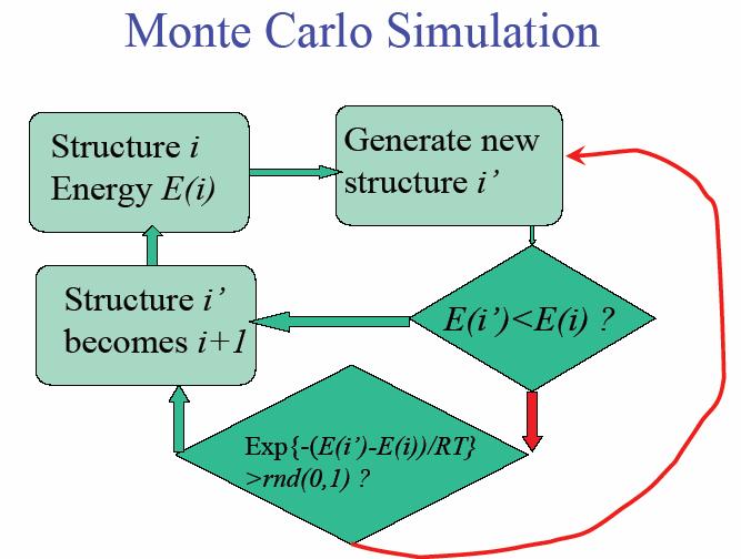
47 Brief Account of MC, MD N ~ ,000 Periodic boundaries Prescribed intermolecular potential Monte Carlo Specify N, V, T Molecular Dynamics Specify N, V, E Generate random moves Sample with P α exp(-υ /kt) Solve Newton s equations F i = m i a i Calculate r i (t), v i (t) Obtain equilibrium properties Take averages Take averages Obtain equilibrium and nonequilibrium properties Monte Carlo Simulation MC techniques applied to molecular simulation, almost always involves a Markov process move to a new configuration from an existing one according to a well-defined transition probability Simulation procedure generate a new trial configuration by making a perturbation to the present configuration accept the new configuration based on the ratio of the probabilities for the new and old configurations, according to the Metropolis algorithm if the trial is rejected, the present configuration is taken as the next one in the Markov chain repeat this many times, accumulating sums for averages taken from D. A. Kofke s lectures on Molecular Simulation, SUNY Buffalo e new βu e old βu State k State k+1 47

48 Differences Between MC and MD MD gives information about dynamical behavior, as well as equilibrium, thermodynamic properties. Thus, transport properties can be calculated. MC can only give static, equilibrium properties MC can be more easily adapted to other ensembles: - µ, V, T (grand canonical) - N, V, T (canonical) - N, P, T (isobaric-isothermic) In MC motions are artificial - in MD they are natural In MC we can use special techniques to achieve equilibrium. For example, can observe formation of micelles, slow phase transitions. 48

49 The Monte Carlo Method In MC simulations the average value is approximated by generating a large number of trial configurations x N using a random number generator, and replacing the integrals by sums over a finite number of configurations. Random sampling: Suppose we choose configurations x N randomly, so the average becomes A = j j ( ) exp U( ) A j j kt exp U ( j) kt Monte Carlo Sampling for protein structure The probability of finding a protein (biomolecule) with a total energy E(X) is: P( X ) = E( X ) exp kt E( Z) exp dz kt Partition function Estimates of any average quantity of the form: A = A( X ) P( X ) dx using uniform sampling would therefore be extremely inefficient. Metropolis and coll. developed a method for directly sampling according to the actual distribution. Metropolis et al. Equation of state calculations by fast computing machines. J. Chem. Phys. 21: (1953) 49

50 Monte Carlo for the canonical ensemble The canonical ensemble corresponds to constant NVT. The total energy (Hamiltonian) is the sum of the kinetic energy and potential energy: E=E k (p)+e p (X) If the quantity to be measured is velocity independent, it is enough to consider the potential energy: A = = E E X k ( p) p( ) A( X )exp exp dxdp kt kt E E X k ( p) p( ) exp exp dxdp kt kt E X A X p( ) ( )exp dx kt E X p( ) exp dx kt The kinetic energy depends on the momentum p; it can be factored and canceled. Monte Carlo for the canonical ensemble Let: P( X ) = E p( X ) exp kt E Z p( ) exp dz kt π ( X Y ) And let be the transition probability from state X to state Y. Let us suppose we carry out a large number of Monte Carlo simulations, such that the number of points observed in conformation X is proportional to N(X). The transition probability must satisfy one obvious condition: it should not destroy this equilibrium once it is reached. Metropolis proposed to realize this using the detailed balance condition: P( X ) π ( X Y ) = P( Y ) π ( Y X ) or π ( X Y ) P( Y ) E = = exp π ( Y X ) P( X ) ( Y ) E kt ( X p p ) 50

51 Monte Carlo for the canonical ensemble There are many choices for the transition probability that satisfy the balance condition. The choice of Metropolis is: E exp π ( X Y ) = 1 ( Y ) E ( X p kt The Metropolis Monte Carlo algorithm: p ) if if E ( Y ) > E p E ( Y ) E p p p ( X ) ( X ) 1. Select a conformation X at random. Compute its energy E(X) 2. Generate a new trial conformation Y. Compute its energy E(Y) 3. Accept the move from X to Y with probability: E p ( Y ) E p( X ) P = min(1, exp kt 4. Repeat 2 and 3. Pick a random number RN, uniform in [0,1]. If RN < P, accept the move. Monte Carlo for the canonical ensemble Notes: 1. There are many types of Metropolis Monte Carlo simulations, characterized by the generation of the trial conformation. 2. The random number generator is crucial 3. Metropolis Monte Carlo simulations are used for finding thermodynamics quantities, for optimization, 4. An extension of the Metropolis algorithm is often used for minimization: the simulated annealing technique, where the temperature is lowered as the simulation evolves, in an attempt to locate the global minimum. 51

What is Classical Molecular Dynamics?

What is Classical Molecular Dynamics? Simulation of explicit particles (atoms, ions,... ) Particles interact via relatively simple analytical potential functions Newton s equations of motion are integrated