ROBOTICS 01PEEQW. Basilio Bona DAUIN Politecnico di Torino

Transcription

1 ROBOTICS 01PEEQW Basilio Bona DAUIN Politecnico di Torino

2 Kinematic Functions

3 Kinematic functions Kinematics deals with the study of four functions(called kinematic functions or KFs) that mathematically transform joint variables into cartesian variables and vice versa 1. Direct Position KF: from joint space variables to task space pose 2. Inverse Position KF: from task space pose to joint space variables 3. Direct Velocity KF: from joint space velocities to task space velocities 4. Inverse VelocityKF: from task space velocities to joint space velocities Remember: pose is the name given to the parameters identifying the position and the orientation of a rigid body A geometrical point has no pose, but only position 3

4 Kinematic functions Direct Position KF: from joint space variables to task space pose This is the pose "vector" p = [ p p p α α α] x y z Inverse Position KF: from task space pose to joint space variables 4

5 Kinematic functions Direct Velocity KF: from joint space velocities to task space velocities Inverse Velocity KF: from task space velocities to joint space velocities 5

6 Kinematic functions Positions and velocities of what? It can be the position or velocity of any point of the robot, but, usually, is the position and velocity of the TCP RF TCP R P BASE R 0? How to compute the homogeneous transformation between these two RF 6

7 Kinematic functions: how to compute them The first step is to fix a reference frame (RF) on each robot arm In general, to move from a RF to the following RF, 6 parameters (three translations of the RF origin + three angles for the RF rotation) are required A number of conventionswere introduced to reducethe number of parameters and to find a common wayto describe the relative position of reference frames Denavit-Hartenbergconventions were introduced in 1955 and are still widely used in industry (with some minor modifications) 7

8 Denavit-Hartenberg conventions The convention defines only 4 parameters between two successive RF, instead of the usual 6, because two constraints are added Joints can be prismatic (P) or revolute (R); the convention is valid in both cases 2 parameters are associated with a translation, 2 parameters are associated with a rotation Three of these parameters depend on the robot geometry only, and therefore are constant in time One parameter depends on the relative motion between two successive links, and therefore is a function of time We call this parameter the i-thjoint variable 8

9 DH convention Assume a connected multibody system with n rigid links The links may not be necessarily symmetric Each link is connected to two joints, one toward the base (proximal), one toward the TCP (distal) RF 1 Base RF 9

10 DH convention Joint 5 Joint 4 Link 3 Joint 6 Joint 3 Link 2 Wrist Link 1 Joint 2 Shoulder Joint 1 Link 0 = base 10

11 DH convention g i + 1 b i + 1 g i + 2 g i bi 1 b i 11

12 DH convention d 1 θ() t q() t

13 DH conventions Rotation of joint 1 only 13

14 DH conventions Rotation of joint 2 only 14

15 DH conventions Rotation of both joints 15

16 DH convention We use the term motion axis to include both revolute and prismatic axes Motion axis Motion axis g i + 1 Motion axis bi gi b i + 1 g i + 2 Base bi 1 symbols b = i g = i arm/link joint We have this sequence b i + 2 TCP 16

17 DH convention 17

18 DH convention Motion axis Motion axis g i +1 g g i + 2 i Motion axis 18

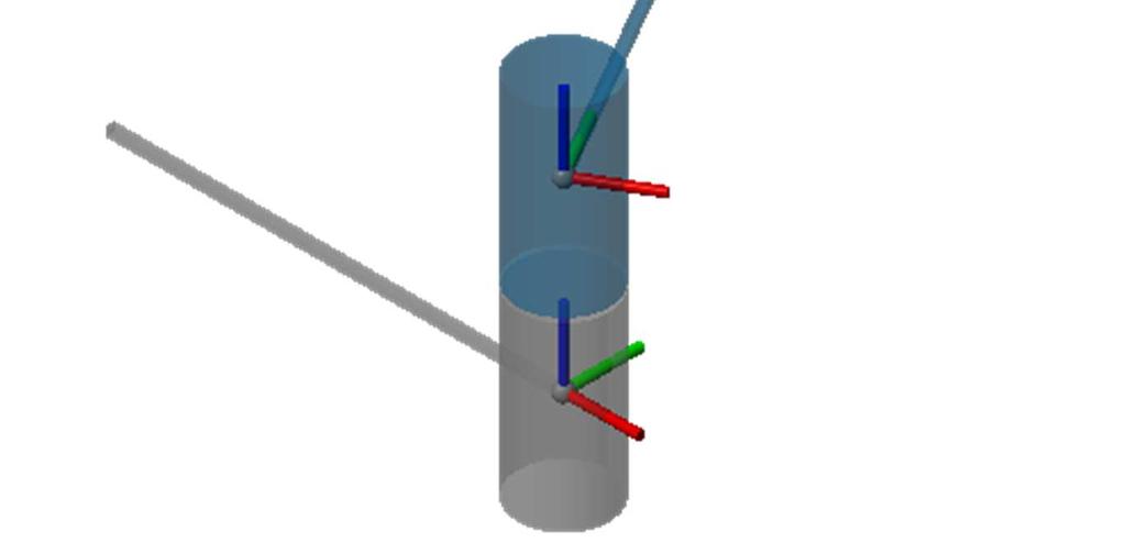
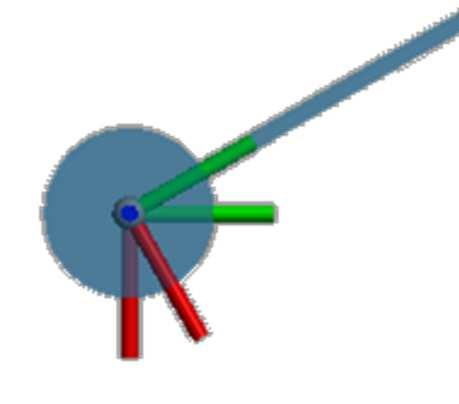
19 DH convention Motion axis g i Motion axis g i +1 Motion axis g i +2 π / 2 π / 2 19

20 DH convention Motion axis g i Motion axis g i +1 Motion axis g i +2 20

21 DH convention Motion axis g i Motion axis g i +1 Motion axis g i +2 21

22 DH convention Motion axis g i Motion axis g i +1 Motion axis g i +2 22

23 DH convention Motion axis g i Motion axis g i +1 Motion axis g i +2 Notice that the origin is not ON g i+1 23

24 DH rules 24

25 DH rules 25

26 DH rules 26

27 Video

28 Video

29 DH parameters DH parameters define the transformation R i 1 R i Depending on the joint type g i Prismatic joint Rotation joint () q () t d t i θ, a, α =fixed i i i i Joint variables Geometrical parameters obtained by calibration () q () t θ t i d, a, α =fixed i i i i 29

30 DH homogeneous roto-translation matrix T TRt R t 0 1 = (,) = T From one reference frame to the next we apply the "pre-post" rule T Trasl(, k )Rot(, k )Trasl(, i )Rot(, iα) i 1 = d θ a i T i 1 i cosθ sinθcosα sinθsinα acosθ i i i i i i i sinθ cosθcosα cosθsinα a sinθ i i i i i i i = 0 sinα cosα d i i i

31 Alternatives to the DH parameters The DH approach is the most common approach to forward kinematics, but it is only one among other conventions. Indeed DH does not handle parallel z-axes very well, and present other drawback when estimating the associated parameters There are various alternatives, including Screw Theory Hayati-Roberts Dual quaternions Although these may (or may not) be better approaches, most of the kinematic libraries accept the DH parameters, and for that reason it is the approach to be considered as first choice. 31

32 Example PUMA robot 32

33 Example PUMA robot 33

34 34

35 Example PUMA robot d = D θ a = q() t = 0 α = 90 k 1 R 1 g 2 g 1 i 1 D 1 k 0 R 0 i 0 35

36 Example PUMA robot D 2 g 2 A 2 g 3 d = D θ a = A α = q() t = 0 k 1 g 1 R 1 i 1 k 2 R 2 i 2 36

37 Example PUMA robot g 3 d = D θ a α 3 = q() t = 0 = 90 R 3 k 2 R 2 i 2 k 3 D 3 R 3 g 4 i 3 37

38 Example PUMA robot From above Lateral view 1 Lateral view 2 38

39 Step-by-step procedure to compute the KF 1 1. Select and numbers joints and links from the base to the TCP 2. Define and place the RF using DH conventions 3. Define the constant DH parameters 4. Define the variable DH parameters generalized coordinate 5. Compute each homogeneous transformation 6. Compute the total 0 T TCP 7. Extract the direct position KF from 8. Compute the inverse position KF 9. Take care of the following problems i 1 i Inverse velocity KF: analytical or geometrical approach Inverse velocity KF: kinematic singularity problem T 39

40 Step-by-step procedure to compute the KF 2 1. Select and identify links and joints 2. Set all RFs using DH conventions 3. Define constant geometrical parameters q 4() t q() t 2 q() t 5 q() t 6 q() t 1 R P TCP BASE R 0 0 T P () () q () q T q = R t P P P T

41 Joint and cartesian variables Joint variables Task/cartesian variables/pose q() t q1() t q2() t q3() t q4() t q5() t q6() t = p() t x1() t x2() t x3() t α1() t α2() t α3() t = position orientation Direct KF ( t ) p() t = f q() Inverse KF q f p ( t ) 1 () t = () 41

42 Direct position KF 1 position q1() t p1() t q2() t p2() t q (()) 3() t p3() t t x q q() t = (()) t q4() t pq = p4() t = q (()) 5() t p5() t t α q q6() t p6() t orientation P P P 1 ( q1) 2( q2) 3( q3) 4( q4) 5 ( q5) 6( q6) R t T = T T T T T T T P = 1 0 T orientation position R = R ( q ()) t = t ( q() ) P P t P P t 42

43 Direct position KF 2 T 0 P 0 0 RP tp = 1 0 T Direct cartesian position KF: easy x x x x t t tp t2 3 3 Direct cartesian orientation KF: not so easy to compute, but not difficult We will solve the problem in the following slides 43

44 Direct position KF 3 (() t) α( q() t) Rq We want to compute angles from the rotation matrix. But it is important to decide the representation to use α ( q() t ) What is? Euler angles RPY angles Quaternions Axis-angle representation 44

45 q (t ) 1 q (t ) 2 x q (t ) ) ( q (t ) p (t ) = f (q (t )) = q (t ) = 3 q 4 (t ) α (q (t )) q 5 (t ) q 6 (t ) The inverse KF is important, since control actions are applied to the joint motors, Inverse position KF 1 while the task to be done is defined in Cartesian space q 3 (t ) Trajectory in space q2 (t ) x q (t ) ) ( α (q (t )) q1(t ) 45

46 Inverse position KF 2 1. The problem is complex and there is no clear recipe to solve it 2. If a spherical wrist is present, then a solution is guaranteed, but we must find it... how? 3. There are several possibilities Use brute force or previous known solutions found for similar chains Use inverse velocity KF (recursive approach) Use symbolic manipulation programs (computer algebra systems as Mathematica, Maple, Maxima,, Lisp) NOT SUGGESTED Iteratively compute an approximated numerical expression for the nonlinear equation (Newton method or others) () t = (() t) ( t) = { pt f( qt) } p f q p() t f q() 0 min () () 46

47 Direct velocity KF 1 Linear and angular direct velocity KF Non redundant robot with 6 DOF q() t p() t ɺ1 ɺ1 q() t p() t ɺ 2 ɺ 2 x q q q() t p() t ɺ ɺ ɺ ɺ q() t p() t ɺ 4 ɺ 4 α q() t p() t ɺ ɺ5 ɺ 5 q() t p() t ɺ6 ɺ6 ((), t () t) 3 3 ɺ() t = pɺ() t = = q ( q(), t qɺ() t) Linear velocity vq q ω ((), t ɺ() t) ( q(), t qɺ() t) Derivative of the angles Angular velocity 47

48 Direct velocity KF 2 A brief review of mathematical notations General rule d pq (()) t dt d (() t) x q dt = d (() t) αq dt d d d ( q ()) = f( q(), t, q(), t, q() t) f t i i 1 j n t dt f i f i f i = j q q q 1 j n qɺ () t qɺ () t qɺ () t n 48

49 Direct velocity KF 3 qɺ () t 1 d f f f (()) i i i f t q() t T q = (() t) () t i j fi dt = q q q ɺ J q qɺ 1 j n q () t ɺn f f f q q q JACOBIAN 1 j n q() t ɺ1 d f f f (()) i i i f qt = q() t (() t) () t j dt q q q ɺ = J q qɺ 1 j n q() t n f f f ɺ m m m q q q 1 j n 49

50 Further notes on the Jacobians Velocity kinematics is characterized by Jacobians There are two types of Jacobians: Geometric Jacobian Analytical Jacobian The first one is related to Geometric Velocities J g J a v p ( ) pɺ() t = J q() t qɺ() t also called Task Jacobian xɺ = = Jqɺ g ω The second one is related to Analytical Velocities pɺ xɺ = = ɺα Jqɺ a 50

51 Geometrical and Analytical velocities What is the difference between these two angular velocities? On the contrary, linear velocities do not have this problem: analytical and geometric velocities are the same vector, that can be integrated to give the cartesian position 51

52 Further notes on the Jacobians Moreover it is important to remember that in general no vector u() t exists that is the integral of ωt ()? u() t ω() t The exact relation between the two quantities is: ( ) ( ) ω() t = θɺ() tu() t + sin θ() tuɺ() t + 1 cos θ() t S u() t uɺ() t While it is possible to integrate when is considered ɺ( τ) () t pɺ( τ)dτ= dτ = ( τ) () t ɺα α x x 52

53 Further notes on the Jacobians The geometric Jacobian is adopted every time the physical interpretation of the rotation velocity is needed The analytical Jacobian is adopted every time it is necessary to treat differential quantities in the task space Then, if one wants to implement recursive formula for the joint position q( t ) = q( t) + qɺ( t) t k+ 1 k k he can use or q 1 ( ) = q( ) + J (( q )) v( ) k+ 1 k g k p k t t t t t q 1 ( ) = ( ) + (( )) ( ) k+ 1 k a k k t qt J qt pɺ t t 53

54 Further notes on the Jacobians Reference 54

55 Geometric Jacobian 1 The geometric Jacobian can be constructed taking into account the following steps a) Every link has a reference frame defined according to DH conventions R i R i b) The position of the origin of is given by: g i g i + 1 R i 1 b i i 1 ri 1, i R i x i 1 x i This is known R 0 x = x + R r = x + r 0 i 1 i i 1 i 1 i 1, i i 1 i 1, i 55

56 Geometric Jacobian 2 Derivation with respect to time gives xɺ = xɺ + R rɺ + ω R r 0 i 1 0 i 1 i i 1 i 1 i 1, i i 1 i 1 i 1, i = xɺ + v + ω r i 1 i 1, i i 1 i 1, i Linear velocity of R wrt R Angular velocity of R i i 1 i 1 Remember: Rɺ = S( ω) R= ω R 56

57 Geometric Jacobian 3 If we derive the composition of two rotations, we have: R = R R Rɺ Rɺ R R R 0 0 i 1 i i 1 i 0 0 i 1 0 i 1 = + ɺ i i 1 i i 1 i 0 i 1 0 i 1 = S( ω ) R R + R S( ω ) R i 1 i 1 i i 1 i 1, i i 0 i i 1 = S( ω ) R R + SR ( ω ) R R i 1 i 1 i i 1 i 1, i i 1 i = ( ω ) ( ω ) S + SR R S( ω) R i 1 i 1 i 1, i i i i Hence: 0 ω = ω +R i i 1 i 1 i 1, i angular velocity of RF i in RF 0 angular velocity of RF i wrt RF i-1 in RF i-1 ω angular velocity of RF i-1 in RF 0 57

58 Geometric Jacobian 4 To compute the Geometric Jacobian, one can decompose the Jacobian matrix as: q LINEAR JACOBIAN ɺ 1 q xɺ L,1 L,2 Ln, 2 3 ( ) J J J ɺ v= = J qqɺ =, g J J R Li, Ai, ω J J J A,1 A,2 An, ANGULAR JACOBIAN q ɺ n J indicates how qɺ contributes to the linear velocity of the TCP Li, i n n dx xɺ = qɺ = J qɺ dq i i= 1 i i= 1 Li, i J A,1 indicates how qɺ contributes to the angular velocity of the TCP i n ω= ω = i 1, i Ai, i i= 1 i= 1 n J qɺ 58

59 Structure of the Jacobian LINEAR JACOBIAN ANGULAR JACOBIAN 59

60 Geometric Jacobian 5 If the joint is prismatic J qɺ = k dɺ ω Li, i i 1 i i 1, i = 0 J = k Li, i 1 J = 0 Ai, R i 1 x i 1 r i 1,TCP R TCP If the joint is revolute J qɺ = ω r = ( k r ) θɺ Li, i i 1, i i 1, TCP i 1 i 1, TCP i ω = k θɺ i 1, i i 1 i J = k r Li, i 1 i 1,TCP J = k Ai, i 1 R 0 x TCP All vectors are expresses in r R ( x x ) is the vector that represents in i 1, TCP TCP i R 60

61 Geometric Jacobian 5 In conclusions, the elements of the geometric Jacobian can be computed as follows: Prismatic Revolute J Li, Ai, i 1 J k 0 k r k i 1 i 1, TCP i 1 61

62 Analytical Jacobian 1 Analytical Jacobian is computed deriving the expression of the TCP pose p(()) t p(()) t q q 1 1 p d (()) t q 1 q q ɺ xq 1 n ɺ 1 dt pɺ = = = d (()) t αq pɺ (()) (()) 6 dt p qt p qt q 6 6 ɺ n q q 1 n J(()) qt a 62

63 Analytical Jacobian 2 The first three lines of the analytical Jacobian are equal to the same lines of the geometric Jacobian The last three lines are usually different from the same lines of the geometric Jacobian These can be computed only when the angle representation has been chosen: here we consider only Euler and RPY angles A transformation matrix relates the analytical and geometric velocities, and the two Jacobians ω=t( ααɺ ) () I 0 J q = () g a ( ) J q 0 Tα 63

64 Relations between Jacobians Euler angles α= { φθψ,, } RPYangles α= { θ, θ, θ} x y z 0 cosφ sinφsinθ T( α) = 0 sinφ cosφsinθ E 1 0 cosθ cosθ cosθ sinθ 0 y z z T ( α) = cosθ sinθ cosθ 0 RPY y z z sinθ 0 1 y The values of α that zeros the matrix T(α) determinant correspond to a orientation representation singularity This means that there are geometric angular velocities that cannot be expressed by joint velocities 64

65 Structure of the Jacobian If the robot is non-redundant, the Jacobian matrix is square If the robot is redundant, the Jacobian matrix is rectangular 65

66 Inverse velocity KF 1 When the Jacobian is a square full-rank matrix, the inverse velocity kinematic function is simply obtained as: ( ) qɺ J q pɺ 1 () t = () t () t When the Jacobian is a rectangular full-rank matrix (i.e., when the robotic arm is redundant, but not singular), the inverse velocity kinematic function has infinite solutions, but the (right) pseudo-inversecan be usedto compute one of them ( ) + qɺ() t = J q() t pɺ() t def + T T 1 J = J ( JJ ) 66

67 Inverse velocity KF 2 If the initial joint vector q(0) is known, inverse velocity can be used to solve the inverse position kinematics as an integral t = + ɺ τ τ + ɺ 0 k + 1 k k q () t q (0) q ( )d q ( t ) q ( t ) q ( t ) t Continuous time Discrete time Assuming that t is small 67

68 Inverse velocity KF 3 If the Jacobian (square or rectangular) is NOT full rank, it is not possible to invert or pseudo invert the matrix using the rule J = J ( JJ ) + T T 1 The solution is given using the Singular Value Decomposition of the Jacobian J= UΣV T and computing the pseudo inverse as + + J = VΣ U T Where + is formed by replacing the non-zero diagonal elements of by its reciprocal 68

69 Singularity 1 A square matrix is invertible if ( ) det J q() t 0 When det J ( q () t ) = 0 S a singularity exists at q () t S This is called a singular/singularity configuration 69

70 Singularity 2 For an articulated/anthropomorphic robot threesingularity conditions exist A. completely extended or folded arm B. wrist center on the vertical C. wrist singularity When joint coordinates approach singularity the joint velocities become very large for small cartesian velocities qɺ = J ( qp ) ɺ= Jpɺ Jpɺ detj ε 70

71 Singularity 3 A. Extended arm The velocities span a dim-2 space (the plane) The velocities span a dim-1 space (the tangent line) i.e., singularity 71

72 Singularity 4 B. Wrist center on the vertical these velocities cannot be obtained with infinitesimal joint rotations 72

73 Singularity 5 C. Wrist singularity Euler wrist RPY wrist Singularity=two axes are aligned Singularity=two axes are aligned 73

74 Euler wrist singularity 3 angles Let us start from the symbolic matrix cc scs cs scc ss φ ψ φ θ ψ φ ψ φ θ ψ φ θ sc + ccs ss + ccc cs φ ψ φ θ ψ φ ψ φ θ ψ φ θ ss cs c ψ θ ψ θ θ cos( φ+ ψ) sin( φ+ ψ) Observe that if = 1 θ= 0 c θ we have cc ss cs sc 0 φ ψ φ ψ φ ψ φ ψ sc cs cc ss 0 + φ ψ φ ψ φ ψ φ ψ angle only 74

75 RPY wrist singularity (from MSMS course) 75

76 Singularity In practice, when the joints are neara singular configuration, to follow a finite cartesian velocity the joint velocities become excessively large Near singularity conditions it is not possible to follow a geometric path and at the same time a given velocity profile; it is necessary to reduce the cartesian velocity and follow the path, or to follow the velocity profile, but follow an approximated path In exact singularity conditions, nothing can be done. So Avoid singularity 76

77 Conclusions Kinematic functions can be computed once the DH conventions are applied Inverse position KF is complex Difference between analytical and geometric Jacobians Inverse velocity can be computed except from singularity points Avoid singularities 77

78 From Robohub web site How to calculate forward kinematics in 5 easy steps 78