MODELING FLUID MECHANICS IN INDIVIDUAL HUMAN CAROTID ARTERIES

Transcription

1 MODELING FLUID MECHANICS IN INDIVIDUAL HUMAN CAROTID ARTERIES A Dissertation Presented to The Academic Faculty by Amanda Kathleen Wake In Partial Fulfillment of the Requirements for the Degree Doctor of Philosophy in the School of Biomedical Engineering Georgia Institute of Technology December 2005

2 Modeling Fluid Mechanics in Individual Human Carotid Arteries Approved by: Dr. Don P. Giddens, Advisor Department of Biomedical Engineering Georgia Institute of Technology Dr. Raymond Vito Department of Mechanical Engineering Georgia Institute of Technology Dr. Marilyn Smith Department of Aerospace Engineering Georgia Institute of Technology Dr. John Oshinski Department of Biomedical Engineering Georgia Institute of Technology Dr. David Ku Department of Mechanical Engineering Georgia Institute of Technology Date Approved: November 28, 2005

3 To William Paul Wake and John Byford

4 ACKNOWLEDGEMENTS First, I owe many thanks to my advisor, Dr. Don Giddens, an inspiring researcher and a patient and kind man. I will always be grateful for the opportunity to learn from someone I respect so greatly. I would like to thank my committee members: Dr. Ku, Dr. Oshinski, Dr. Smith, and Dr. Vito. I truly appreciate their advice, suggestions, time, and encouragement. In particular, Dr. Oshinski has cheerfully scanned and rescanned data for me. I would like to acknowledge the National Science Foundation and the Medtronic Foundation for funding I received while working on my degree. In addition, I would like to give respek to Dr. Allen Tannenbaum, who has been infinitely more kind than was necessary. He has generously lent his programs, his lab space, and his ear to aid in my project. While at Georgia Tech I have had the great fortune to have been surrounded by many wonderful people, some of whom deserve special thanks for the entertainment and guidance which they have provided: Dr. Cecilia Curry, Dr. Jimmy Costello, Dr. Eli Hershkovits, Dr. Patricio Vela, Dr. Dan Karolyi, Dr. Tim Healy, Dr. Dave Frakes, and Dr. Kerem Pekkan. The IBB and BME support staffs have been phenomenal; I would like to thank Joanne Wheatley, Chris Ruffin, Pat Thomas, Gail Jefferson, Shauna Durham, Rachel Arnold, Jonathan Glass, and Steven Marzec. I am grateful for Delphine Nain, Dr. Marc Niethammer (without whose help I would still be connecting dots), and Dr. Eric Pichon, who have been such fun and helpful cubicle mates. I owe special thanks to the Tannenbaum lab for their help and iv

5 camaraderie, especially Dr. Lei Zhu, Yan Yang, and Jimi Malcolm who provided additional technical assistance. I owe many thanks to Rina, Allen, Sarah, and Manny Tannenbaum and Jackie, Leo, and Little Leo White for their help, hospitality, and friendship. I would also like to thank Tirza Kramer, Leslie and Mark Henderson, and Lee Sugg for being friends who have transcended time and space. Finally, I am most grateful for the support of my dear family: Sandra Wake, Matthew Wake, Nathan Wake, and Mary Byford. I wish to thank my mother for the patience and understanding she displayed, the encouragements she offered, and the sacrifices she made during the years of study leading to this thesis, (Wake, 1972). My mother has been a tireless cheerleader throughout this entire process and a patient editor to the end. Since childhood my brothers have been wonderfully fun, and they have let me tag along with them; Matt has blazed trails for me, and Nath has given me wise counsel. My grandmother, Mary Byford, has been incredibly generous with her time and resources. I am fortunate to call them my family, and I am proud to call them my friends. v

6 TABLE OF CONTENTS Page ACKNOWLEDGEMENTS LIST OF TABLES LIST OF FIGURES LIST OF SYMBOLS SUMMARY iv ix x xiii xv CHAPTER 1. Introduction Plaque etiology Fluid dynamics and vessel response Investigating the flow field in arteries 9 2. Methods Model construction Data acquisition Segmentation and surface reconstruction Computational volume Discretization Solution Validation Steady flow Grid sensitivity Subject-specific models Application of boundary conditions 35 vi

7 Comparison with Womersley boundary conditions Results Subject-specific models Comparison with PCMR data Velocity profiles Negative axial velocity regions Wall shear stress Womersley model Comparison with PCMR data Velocity profiles Negative axial velocity regions Discussion and Conclusions Inlet velocity distributions affect negative axial flow patterns Inlet velocity distributions affect negative axial flow location Location of lowest axial wall shear stress is subject-specific Limitations MRI Registration of PCMR to MR data Flow split estimation Velocity measurement Modeling assumptions Conclusions 81 APPENDIX A: Phantom Model Details 83 APPENDIX B: Grid Sensitivity 86 vii

8 REFERENCES 89 VITA 98 viii

9 LIST OF TABLES Table 1: Geometry scan parameters 20 Table 2: Flow parameters for steady state simulations 32 Table 3: Outflow ratios of the internal carotid artery to the external carotid artery (IC:EC) for steady state simulations 32 Table 4: Comparison of diameters at key positions of the phantom 34 Table 5: PCMR scan data 36 Table 6: Data acquisition times (s) for Model A at each PCMR plane 43 Table 7: Data acquisition times (s) for Model B at all PCMR planes 43 Table 8: Average axial velocity differences between PCMR measurements and CFD calculations for Model A 48 Table 9: Average axial velocity differences between PCMR measurements and CFD calculations for Model B 48 Page ix

10 LIST OF FIGURES Figure 1: Sylgard phantom based on the model developed by Balasubramanian 21 Figure 2: Reconstruction of the phantom model 27 Figure 3: Computational volumes of Model A and Model B 28 Figure 4: Meshing the bifurcation region 29 Figure 5: At RE=400, the CC-IC recirculation grows as flow through the external carotid branch increases 34 Figure 6: Velocity profiles in the plane of bifurcation for RE=400, IC:EC=70:30 34 Figure 7: Verification that PCMR data is aligned with finite element nodes 37 Figure 8: Common carotid inlet of Model A and a circle of radius, R= m 39 Figure 9: Computational geometry of Model A with the axial locations of the PCMR data planes 42 Figure 10: Computational geometry of Model B with the axial locations of the PCMR data planes 42 Figure 11: Volumetric waveform (m 3 /s) for Model A 44 Figure 12: The proportion of flow through the internal carotid outlet for Model A 44 Figure 13: Volumetric waveform (m 3 /s) for Model B 44 Figure 14: The proportion of flow through the internal carotid outlet for Model B 45 Figure 15: Comparison of axial velocity (m/s) for Model B at CC 1 at t 6 46 Figure 16: Comparison of axial velocity (m/s) for Model A at CC 2 at t 2 49 Figure 17: Comparison of axial velocity (m/s) for Model A at CC 2 at t 5 49 Figure 18: Comparison of axial velocity (m/s) for Model A at CC 2 49 Figure 19: Comparison of axial velocity (m/s) for Model B at CC 2 at t 3 50 Figure 20: Comparison of axial velocity (m/s) for Model B at CC 2 at t 6 50 Figure 21: Comparison of axial velocity (m/s) for Model B at CC 2 at t Page x

11 Figure 22: Comparison of axial velocity (m/s) for Model B at CC 2 at t 9 51 Figure 23: Comparison of axial velocity (m/s) for Model B at BI 2 at t Figure 24: PCMR data from Subject B at BI 1 and at BI 2 52 Figure 25: Skewing of the Model A velocity profile towards the internal carotid 53 Figure 26: Skewing of the Model B velocity profile towards the external carotid 53 Figure 27: Axial velocity contours of the Model A inlet plane at t 1 -t Figure 28: Axial velocity contours of the Model B inlet plane at t 1 -t Figure 29: Regions of negative axial flow of Model A at t 1 -t Figure 30: Extent of negative axial flow subregion through the external carotid in Model A at t 1 -t Figure 31: Regions of negative axial flow of Model B at t 1 -t Figure 32: Average axial wall shear stress for Model A 61 Figure 33: Average axial wall shear stress for Model B 62 Figure 34: Axial velocity distributions at CC 1 at t 1 -t 5 for Model A and for Model W 63 Figure 35: Negative axial velocity regions at t 1 -t 5 for Model A and for Model W 66 Figure 36: Extent of NAVR at t 2 and t 5 of Model A 66 Figure 37: Extent of NAVR at t 2 and t 5 of Model W 66 Figure 38: At t 2 inlet axial velocity profiles and negative axial flow regions in Model A and Model W 67 Figure 39: At t 3 inlet axial velocity profiles and negative axial flow regions in Model A and Model W 67 Figure 40: At t 4 inlet axial velocity profiles and negative axial flow regions in Model A and Model W 68 Figure 41: At t 5 inlet axial velocity profiles and negative axial flow regions in Model A and Model W 68 Figure A.1: Location of comparison planes of the phantom model 84 Figure A.2: For a constant flow ration, IC:EC=70:30, the recirculation region grows as the Reynolds number increases 85 xi

12 Figure A.3: Velocity profiles in the plane perpendicular to the plane of bifurcation for RE=400, IC:EC=70:30 85 Figure B.1: The axial velocities at the common carotid measurement planes for the standard mesh and for the finer mesh at RE=400, IC:EC=70:30 87 Figure B.2: The axial velocities at the internal carotid measurement planes for the standard mesh and for the finer mesh at RE=400, IC:EC=70:30 88 Figure B.3: The axial velocities at measurement plane CCA4 88 xii

13 LIST OF SYMBOLS f dv f i J 0 (xi 3/2 ) Euclidean arc length of active contour Frequency Body force per unit volume Bessel function, order zero L φ (t) Length functional of active contour N p Q R r RE t U u i w x i α δ ij κ Unit inward normal Pressure Volumetric flowrate Maximum radius Radius Reynolds number Time Average axial velocity Velocity Axial velocity Position Womersley parameter Kronecker delta function; δ ij = 1 if i=j and δ ij = 0 if i j Curvature term µ Viscosity coefficient ν ρ Dynamic viscosity Density xiii

14 σ ij φ Stress tensor Conformal term xiv

15 SUMMARY In the interest of furthering the understanding of hemodynamics, this study has developed a method for modeling fluid mechanics behavior in individual human carotid arteries. A computational model was constructed from magnetic resonance (MR) data of a phantom carotid bifurcation model, and relevant flow conditions were simulated. Results were verified by comparison with previous in vitro experiments. The methodology was extended to create subject-specific carotid artery models from geometry data and fluid flow boundary conditions which were determined from MR and phase contrast MR (PCMR) scans of human subjects. The influence of subject-specific boundary conditions on the flow field was investigated by comparing a model based on measured velocity boundary conditions to a model based on the assumption of idealized velocity boundary conditions. It is shown that subject-specific velocity boundary conditions in combination with a subject-specific geometry and flow waveform influence fluid flow phenomena associated with plaque development. Comparing a model with idealized Womersley flow boundary conditions to a model with subject-specific velocity boundary conditions demonstrated the importance of employing inlet and flow division data obtained from individual subjects in order to predict accurate, clinically relevant, fluid flow phenomena such as low wall shear stress areas and negative axial velocity regions. This study also illustrates the influence of the bifurcation geometry, especially the flow divider position, with respect to the velocity distribution of the common carotid artery on the development of flow characteristics. Overall it is concluded that accurate geometry and velocity xv

16 measurements are essential for modeling fluid mechanics in individual human carotid arteries for the purpose of understanding atherosclerosis in the carotid artery bifurcation. xvi

17 1. Introduction Worldwide, more than 16 million people die each year due to cardiovascular disease, more than 5.5 million of which were attributed to strokes in 2002 (World Health Organization, 2004). In 2001 more than 20 million people suffered strokes, 5.5 million of which were fatal (World Health Organization, 2002). In the United States 60.8 million people have at least one type of cardiovascular disease, the leading cause of death. Of these, 4.5 million people have suffered strokes, with approximately 600,000 strokes occurring each year (American Heart Association, 2001). Both stroke and transient ischemic attack can result from thrombolytic and embolytic complications of arteriosclerosis in the common carotid or the internal carotid arteries. Atherosclerotic plaques, a manifestation of arteriosclerosis, include fatty streaks (lipids and foam cells); gelatinous plaques (collagen fibers around small lipid droplets); and fibrous plaques (fibrous caps containing smooth muscle cells over a core of cholesterol esters). Numerous in vivo, in vitro, and numerical experiments have been conducted to understand the development of atherosclerosis, and these efforts have produced many theories on atherogenesis and atherosclerosis development including a cellular response to lipids, a thrombogenic response to molecules in blood, an unchecked healing response to endothelial layer injury, a cancer-like proliferation of smooth muscle cells, chronic inflammation, and a hemodynamic effect on the arterial cells (DePalma, 1997). By understanding the mechanisms by which a plaque will initiate, grow to 1

18 occlude the lumen, rupture, or remain stable, clinicians will be better able to predict how a plaque might develop or react to treatment. Insight will provide a better basis from which patients and clinicians can select options for treatment of plaques, whether by arterial bypass, by angioplasty, by stenting, or by other therapy. The involvement of hemodynamics, the basis for the approach of this work, is supported by the characteristic location of atheroma in particular vasculature (e.g., carotid arteries, coronary arteries, popliteal arteries), and, specifically, the location of plaques at preferential positions within those arteries. Typically, the localized plaques occur at geometric structures (e.g., branch points, bifurcations, and curves), which produce fluid dynamics patterns (e.g., low wall shear stress, recirculation regions, and secondary flows) that colocalize with atherosclerosis development (Tropea, et al., 1997) Plaque etiology Since the artery is a responsive tissue, not an inert conduit, it is useful to examine the structure and behavior of the vessel, at least cursorily. For the artery of concern, the carotid artery, there are three distinct strata: intima, media, and adventitia. The outermost layer, the adventitia, consists of collagen fibers, fibroblasts, macrophages, nerves, and blood vessels, and it tethers vessels to the surrounding tissue. The next layer inward is the media, which is composed of smooth muscle cells, elastin, collagen, and proteoglycans. The adventitia and especially the media are the layers which contribute to the mechanical behavior of the vessel. Finally, the innermost layer, the intima, is on the lumen side of the vessel and contains the endothelial layer and a basal lamina. The intima, especially the endothelial layer, provides control over the wall permeability to 2

19 substances in the blood (i.e., proteins, fats, leukocytes) and resistance to thrombosis (Fung, 1993). Bulk flow environments affect the genesis and development of atherosclerosis through various mechanisms via interaction with the endothelial layer as transducer and as barrier. In this section a brief description of select plaque development mechanisms is offered. Except where specifically noted in this section, plaque etiology is summarized from a review article (Lusis, 2002), which describes the process in great detail. Briefly: 1. Lipoproteins breach the endothelium. 2. Once in the intima low density lipoprotein (LDL) is modified, whereupon it induces local endothelial cells to attract monocytes to the vessel wall. 3. Modified LDL interrupts normal vascular compensatory mechanisms. 4. Leukocytes infiltrate the vessel, proliferate, and differentiate, finally ingesting lipoproteins to result in foam cells. 5. Smooth muscle cells (SMC)s migrate into the intima, proliferate, and produce extracellular matrix. In addition to being a transducer of stress and strain (induced by blood flow) into biochemical signals, the endothelial layer functions as the artery s barrier to blood borne particles. LDL, among other lipoproteins, diffuses across the endothelium into the intimal layer. As systemic levels of LDL increase, the level of accumulation of LDL in the intima increases. The review by Dejana et al., (1997), concludes it is possible the permeability of the layer is affected by inflammatory agents bound to receptors. Once 3

20 bound, the receptors signal for cytoskeletal reorganization and the opening of endothelial cell-cell gaps. Once in the intima LDL is modified in several ways. When LDL undergoes oxidation by reactive oxygen species (ROS), it induces local endothelial cells to produce molecules (e.g., growth factors, adhesion molecules), which facilitate the binding of circulating monocytes to the vessel wall. Monocyte adhesion has been modeled in vitro to test the influence of varying flow fields. For steady flow in an in vitro study, cell adhesion varied inversely with shear stress in areas where cells were close to the model wall; however, under pulsatile flow conditions cell adhesion was not localized in areas of low wall shear stress (Hinds et al., 2001). Furthermore, oxidized LDL interrupts normal vessel regulatory mechanisms by inhibiting nitric oxide (NO) production. NO, involved in vasodilation, helps to guard against atherosclerosis development. After monocytes infiltrate the wall, growth factors such as macrophage colonystimulating factor (M-CSF) are produced by endothelial cells via inducement by oxidized LDL. These growth factors encourage macrophages to proliferate and to differentiate. After substantial modification by several enzymes and ROS, LDL is altered such that when ingested by macrophages, foam cells are formed. As these foam cells die their contents accumulate to form pools of extracellular lipids and debris, which can eventually contribute to the necrotic core of advanced lesions. High density lipoproteins (HDL) interrupt the formation of foam-cells as well as transport cholesterol from the tissue into the bloodstream. As the necrotic core grows it is covered by a fibrous cap formed from the accumulation of SMCs and their extracellular matrix. Smooth muscle cells migrate from 4

21 the media into the intima, proliferate, and produce extracellular matrix in response to cytokines and growth factors expressed by endothelial cells, macrophages, and T-cells in the intima. Platelet-derived growth factor (PDGF), the endothelial cell concentration of which increases with low shear stress, encourages SMC migration into the intima, and it is a vascular SMC growth factor contributing to intimal thickening (Mondy et al., 1997; Owens, 1995). Arteries experience nonlinear, large deformations, and early and late stage plaques influence the stress distributions in the wall. Areas of significant thickening, especially areas with plaque, correlate with a nonlinear increase in carotid artery wall stiffness (Labropoulos et al., 2000). Salzar et al., (1995), reported mechanical stress varies over a model of the carotid bifurcation, with the highest stress concentrations at the bifurcation and across the sinus bulb. Finite element models (FEM)s of histological arterial cross sections showed that incidence of plaque rupture corresponded with segments experiencing high circumferential stress, and a compliant model indicated areas of high tensile stress coincided with areas of low wall shear stress (Zhao et al., 2000). In FEMs of focal plaques with nonlinear mechanical properties, tensile stress maximums were reported near the plaque edge (Hayashi and Imai, 1997). However, site rupture did not always correspond with the location of maximum stress, thus indicating the influence of the ever-changing biomechanical environment and the three-dimensional nature of plaque in situ (Cheng, 1993). Plaques can continue to grow and develop, become quiescent, or rupture; the composition of a plaque influences its behavior; its vulnerability is affected by calcification and vascularization, and its thrombogenicity is affected by its protein 5

22 constituents. Modeling heterogeneities within atherosclerotic arterial wall components (e.g., disease-free artery, fibrous plaque, lipid pool, and calcified regions) indicates that stress distribution and magnitude are influenced by the shape and the composition of the fibrous plaque (Beattie et al., 1998). Further, it has been reported that the material property differences within the arterial wall caused by plaque development have more influence on wall stress than the geometry changes of the plaque (Vito et al., 1990; Beattie et al., 1999). Vulnerable plaques become more susceptible to rupture as the fibrous cap thins due to the growth/remodeling of the extracellular matrix by substances secreted by leukocytes within the intima. Monocytes, macrophages, and lymphocytes generate metalloproteinases, which degrade collagen, a structural component of fibrous plaques (Welgus et al., 1990; Galis et al., 1994). Rupture of the plaque often occurs at the shoulders of the plaque where there is an accumulation of foam-cells. Plaque shoulder and core areas demonstrated increased matrix metalloproteinase (MMP) expression, and elevated amounts of matrix metalloproteinase-1 (MMP-1) were found at locations of finite element modeled high circumferential stress (Lee et al., 1996) Fluid dynamics and vessel response Atherosclerotic lesions occur characteristically at particular locations of the arterial tree. These sites have recurring geometrical themes including branching vessels, bifurcations, and curves. These structures generate flow phenomena implicated in atherosclerotic development: low or varying wall shear stress, secondary flows, and separated flows (e.g., Tropea et al., 1997). 6

23 Endothelial cells, which line the wetted surface of the artery wall, are mechanotransducers, transferring fluid dynamics stresses imposed by the blood into biochemical signals of the vascular cells. One theory of signal transduction is that the stiffness of the membrane itself serves as a sensor of wall shear (Knudsen and Frangos, 1997). The range of mean wall shear stress is dynes/cm 2 for many mammalian arteries under normal flow conditions (Giddens et al., 1990). Arteries respond to transient or long term deviations from normal flow conditions through vasodilation/vasoconstriction or by vessel remodeling, respectively (Kamiya and Togawa, 1980; Zarins et al., 1987; Tropea et al., 1997). Chronic changes in blood flow trigger a compensatory mechanism in arteries. Increases in flow result in remodeling of the arterial wall to increase lumen diameter and thus to maintain wall shear stress levels within the normal wall shear stress range, suggesting a coupling between blood flow and artery wall behavior (Zarins et al., 1987). Local fluid mechanics directly affect atherosclerosis initiation and progression. Low and oscillatory wall shear stress regions were found to correspond to atheroma locations (Zarins et al., 1983; Ku et al., 1985; He and Ku, 1996). In the carotid bifurcation minimal intimal thickness was found at the flow divider, an area of high wall shear stress, and the maximum thickness was found on the outer wall of the carotid sinus where complex flow patterns and separation regions were seen (Zarins et al., 1983). In the common carotid artery and distal portions of the internal carotid artery intimal thickening was uniform and minimal; however, at the level of the bifurcation the internal carotid artery tends to exhibit atherosclerosis (Zarins et al., 1983; Ku, 1983), although plaques can also occur in the external carotid artery, as well. Numerical modeling of the 7

24 progression of intimal thickening in low shear regions produced a remodeled geometry with a more even distribution of wall shear stress (Lee and Chiu, 1996). Plaques continue to grow radially outward, the arteries expanding to maintain a lumen diameter, until a critical point is reached, whereupon, the plaque begins to obstruct the lumen (Bond et al., 1981). Patients with carotid artery occlusion have an increased risk of stroke when the occlusion advances more rapidly than the compensatory mechanism of arteriole vasodilation (Grubb et al., 1998). In the common carotid artery, increases in intimal-medial thickness (IMT) are related to the presence and severity of atherosclerotic plaques (Bonithon-Kopp et al., 1996; Hallerstam et al., 2000). Above the threshold value of IMT=0.75 mm, the risk of stroke increases with IMT (Aminbakhsh and Mancini, 1999). Plaques themselves can be asymptomatic until there is significant area reduction, but catastrophe can occur earlier as a thrombolytic or an embolytic event triggered by plaque rupture. Since blood is a multiphase fluid and the vessel wall is selectively permeable, mass transfer can be altered by near wall flow patterns. The permeability of the endothelial layer and mass transport in the endothelial layer vicinity are associated with the early stages of atherosclerosis. The endothelial layer is more permeable in regions of branches and curves, where the endothelial cell shape is more polygonal, than in areas of laminar, unidirectional flow, where the endothelial cells are aligned with the flow (Gimbrone, 1999). Recirculation regions increase particle residence time in proximity to a wall; the carotid sinus is an expansion area, which under pulsatile flow potentially becomes a separation region, allowing blood borne cells and molecules a longer time for mass transport into the vessel wall (Giddens and Ku, 1987). Ma et al., (1997) suggest 8

25 that regions with low mass transfer of small particles may correlate with areas of low intimal thickening. Further, Rappitsch and Perktold (1996) found that wall flux in a shear-dependent permeable model showed flux minima at flow separation and at the reattachment point; however, wall flux in a constantly permeable model was relatively constant spatially Investigating the flow field in arteries Fluid mechanics modeling can be approached experimentally, theoretically, or numerically. Fluids experiments are restricted by physical limitations (e.g., equipment, measurements) and instrumentation; however, in flow experiments complex geometries can be modeled, and complex physics phenomena (e.g., turbulence) potentially have better representation in in vitro experiments than in the other two approaches. In theoretical models equations governing the system are defined. Simplifying assumptions on the physical nature of the situation are made to construct a solvable problem, often limiting this approach to simple systems (geometrically and physically); however, broad understanding is conveyed in a concise, mathematical form. Computational fluid dynamics (CFD) modeling often entails assumptions on the nature of the problem in order to solve the equations defining the problem, but complicated geometries can be accommodated. Numerical models are primarily limited by computational resources and by the understanding of the physical nature of the problem (Tannehill et al., 1997). In numerical modeling decisions on the modeling parameters (e.g., fluid properties, boundary conditions) potentially impact the simulation quality. Reducing the model complexity can result in reduced solution time; however, the speed increase must 9

26 be balanced against the cost to the quality of solution. Two long disputed simplifications in artery models (both in vitro and numerical) are discussed here: the Newtonian fluid assumption and the use of compliant walls. Blood is a multiphase fluid, with the primary particle constituent being red blood cells. A shear-thinning fluid, blood becomes decidedly non-newtonian when flowing through small vessels where the size of red blood cells is on scale with the vessel (Ku, 1997). However, in large arteries shear rates are sufficiently high and the length scale is large enough to approximate blood as a Newtonian fluid (Caro et al., 1978; Strony et al., 1993). In both an experimental and a numerical model of low Reynolds number flow in an averaged carotid bifurcation, Gijsen et al., (1999), found differences in axial velocity profiles and in the prevalence of secondary flow for different viscosity models. Further, they found that slight differences in shear rate control the effect of Newtonian flow on the velocity distribution, accounting for discrepancy between findings of the influence of the Newtonian fluid assumption. Using the classification system proposed by Tang et al., (2004), implementing the assumption that flow in arteries is Newtonian in nature is on the lowest order, Level III, of impact of the simplification on computational results. Differing opinions also exist on the importance of modeling arterial flow with compliant or rigid walls. Real arteries are tethered in situ; hence, there are small axial deformations, but there are appreciable circumferential changes with pressure. Comparisons between geometrically identical, compliant and rigid models of a largescale averaged human carotid bifurcation with the same flow waveform illuminate differences of wall motion, mean wall shear stress, peak wall shear stress, and separation points (Anayiotos et al., 1994; Anayiotos, 1990), but the authors suggest that these 10

27 differences are not major. Although Perktold et al., (1994), concluded that compliance was not as important hemodynamically as differences in individual geometries, they reported flow recirculation regions and peak wall shear stress values were altered by the consideration of compliance in the model. A geometric approximation of the Balasubramanian model (Balasubramanian, 1980) was reproduced and modeled under both rigid and compliant boundary conditions (Reuderink, 1991). Reuderink reported that wall deformation correlated with cross-sectional lumen area and that the compliant model demonstrated smaller recirculation regions and lower wall shear stresses near peak systole than the rigid model. Further, the numerically simulated reverse flow region developed at the deceleration of the flow waveform, contrary to the reports that describe the development of the recirculation region as forming just prior to peak systole (e.g., Perktold et al., 1994; Reuderink, 1991). The explanation of Reuderink for the time of reversed flow development is given as a pseudo-capacitance of the compliant model. As the flow accelerates the model distends and higher velocities are seen in the distal internal carotid. As the flow decelerates flow separation occurs at the sinus (Reuderink, 1991). Using a geometry based on the reports of Ku et al., (1985) but employing an alternative pressure wave form, Perktold and Rappitsch (1995) reported differences between compliant and rigid wall models. The bulk flow patterns were consistent between the two models, but quantitatively they showed differences. Along the internal carotid during the acceleration phase of systole, the compliant model showed lower axial flow velocity than the rigid model (when the vessel expands); however, during the deceleration phase, the compliant model showed higher axial velocity than the rigid model (when the compliant vessel contracts). The compliant model has smaller 11

28 recirculation regions, a lower magnitude of negative axial velocity, and smaller secondary velocities. At the side wall flow separation is greater in the distensible model, with a longer reversed flow region length, but at the outer sinus wall the separation region is smaller in the compliant model than in the rigid model. For some periods of the pulsatile cycle, reversed flow is only seen in the rigid model. Further, the compliant model showed lower wall shear stress values than the rigid model, especially at the divider wall of the internal carotid artery near the bifurcation region. Maximum displacement occurs in the bifurcation region at the side wall, which happens to be a zone of low principal stress at the inner surface of the wall, and normal displacements are much greater than tangential displacements. Again referring to the classification by Tang et al., (2004), the effect of solid mechanics inclusion with fluid mechanics models is a Level II factor, indicating much greater influence on the result than considering non- Newtonian behavior. For the purposes of the current study, the fluid is considered an incompressible, single phase, non-reacting, Newtonian fluid, which flows in a rigid artery in the laminar flow regime. Although blood is not strictly Newtonian and arteries are not rigid, these assumptions are made for model simplicity and must be considered when analyzing results. A method for modeling the fluid mechanics in individual human carotid arteries was developed which involves obtaining data from normal subjects and producing subject-specific numerical models of the flow field in the carotid bifurcation. A series of experiments performed on a large-scale carotid bifurcation geometry was selected for a validation case. Finally, two models were developed from normal subjects using 12

29 measured geometry and spatially and temporally variant velocity boundary conditions. One of those models was used to investigate the influence of subject-specific boundary conditions by also applying an idealized form of velocity boundary conditions and comparing the flow field results with those obtained by using the actual measured values. 13

30 2. Methods In order to investigate the importance of subject-specific boundary conditions of the carotid artery bifurcation, finite element models were developed from clinical imaging modalities. To conduct a finite element analysis the computational geometry of the flow field under investigation is defined; the boundary conditions are assigned; and the equations describing the system are solved numerically. Computational geometry development consists of five stages: data acquisition, segmentation, surface reconstruction, computational volume construction, and discretization. In this study the geometry data for all models are obtained via magnetic resonance imaging (MRI); the images are segmented to determine the shape of the lumen; and a computational grid of the fluid domain is constructed. For the phantom model the velocity boundary conditions are assigned to be consistent with in vitro experiments, and for the human models phase contrast MR (PCMR) data are obtained for the velocity conditions. Fluid dynamics simulations of these models were conducted using a commercially available finite element code, FIDAP (Fluent, Inc., Lebanon, NH), and post-processing was done in Tecplot (Tecplot, Inc., Bellevue, WA) Model construction In a human artery model, obtained by averaging over a number of subjects, areas of interest can be smoothed, consequently eliminating differences of local geometry 14

31 between patients and affecting wall shear stress and secondary flow (Moore et al., 1998; Milner et al., 1998; Perktold et al., 1994). Rigid models of an individual human bifurcation demonstrated variability of secondary flows with geometry, and differences in vessel geometry were shown to impact bifurcation model results more than the inclusion of vessel compliance in a model (Zhao et al., 2000; Perktold et al., 1994). Therefore, obtaining accurate geometry information is vital for individual model construction Data acquisition Several methods including optically digitizing casts from cadavers, ultrasound (US), x-ray angiography, computed tomography (CT) scans, and MRI have been used to determine carotid geometries and boundary conditions from patients (Botnar et al., 2000; Balasubramanian, 1980; Oyre et al., 1998; Moore et al., 1999a; Moore et al., 1999b; Moore et al., 1998; Chandran et al., 1996; Long et al., 2000; Fessler and Macovski, 1991). Geometries for numerical models of carotid bifurcations have been developed from casts of vessels and from fixed vessels (e.g., Botnar et al., 2000, Moore et al., 1999b). The process by which the vessels are cast or fixed can introduce inaccuracies of vessel measurements and of the three-dimensional configuration of the model (Moore et al., 1999b). Ultimately, since we are dealing with normal human volunteers, using casts of excised vessels is not an option. In ultrasound measurements acoustic signals are used, the returning signals of which vary with the mechanical properties (e.g. density, elasticity) of tissues. Resolution in-plane (0.3-3mm) depends on signal frequency and depth of measurement. The range 15

32 of measurement depth depends on the frequency of the signal, but can vary from 3-25 cm. These resolution limits can be improved by using transducers inside the body (e.g., transesophageal transducer). US is a cheap, portable, and, unless an internal transducer is used, non-invasive imaging modality. The acoustic waves used are safe, having been studied and adapted extensively enough to avoid the possible damaging mechanisms of cavitation and heating (Szabo, 2004). X-rays are light waves with wavelength less than 1Å. The x-rays go through the body, and different tissues absorb the energy at different rates. The sensor (film) detects the sum total of energy which has been attenuated in the body and projects in two dimensions the tissue which the rays have passed through in the direction normal to the sensor. Resolution (approximately 1mm) is a function of which tissues the x-rays have traversed (i.e., how much energy has been lost) and the width of the x-ray beam. Although widely used to image bone and air pockets, the standard x-ray method of imaging cannot distinguish between different soft tissues; it can be used for vessel imaging if radioactive contrast agents are used. Even for these angiograms at least two orthogonal images need to be obtained in order to extrapolate any three-dimensional information. The biggest concern with x-ray use is the exposure to radiation (Szabo, 2004). Computed tomography uses multiple x-ray measurements which are taken from different orientations (e.g. planar or helical trajectory of measurement) with respect to the subject via an x-ray source which produces more than a point-source of energy. The x- rays pass through the body and are collected by an array of sensors; then the source and sensor configuration move. As discussed in the previous paragraph, in standard x-ray 16

33 images the differences between soft tissue types are not observed; however, with CT, there is a sufficiently large data set to allow the detection of the signal variance among tissues. Mathematically reconstructing the attenuation of the x-ray data sets provides a representation of the tissues within a cross-section of the subject. Although the large number of measurements allows differentiation between tissues, it also increases the subject s exposure to radiation. Resolution is sub-millimeter, and the system is significantly more expensive than standard x-rays (Szabo, 2004). Relevant to fluid mechanics modeling there is no method for obtaining blood flow measurements with CT, requiring a second mode of imaging to acquire data necessary for constructing subjectspecific models. Magnetic resonance imaging is the most expensive of the imaging modalities discussed here. There are different scan protocols, but the most basic description follows. MR aligns spinning nucleic protons (most commonly hydrogen) with a magnetic field. The hydrogen protons in each tissue rotate at an intrinsic frequency. A radio frequency pulse in a plane orthogonal to the magnetic field is applied at a frequency identical to that of the spinning protons. This excites the protons. After the duration of the pulse, the spinning of the protons are coordinated, thus creating a rotating magnetic pulse, which generates a signal. As the excited protons return to their pre-pulse state the emitted signal is sensed by coils, and properties (typically, longitudinal magnetization and transversal magnetization) are sensed over time to determine time constants (T 1 and T 2, respectively). T 1 and T 2 identify the tissue type and are used for constructing the image. The result is a three-dimensional description of the internal structures of the subject. Often this data set is represented as a series of two dimensional slices along an axis 17

34 (similar to a sliced hotdog). The characteristics of the magnetic field (e.g., magnet strength and coil type) dictate the resolution of the images, but in-plane resolution is less than 1mm (Schild, 1990; Szabo, 2004). Contrast agents can be used to increase the signal of substances, but good quality images can be obtained without them. Although the imaging modality is safe, there are a few limitations such as patients should not be claustrophobic, nor have metal in their bodies (e.g., plates, screws, pacemakers). Another advantage of MR is that both geometry and velocity data can be accrued at the same time and in the same scanner with magnetic resonance scans. In regions of simple flow in vitro MR measurements had very high precision and in vivo measurements demonstrated very high repeatability (Chatzimavroudis et al., 2001). One method of measuring velocity is PCMR. Botnar et al., (2000) found that peak axial velocities vary less than 10% between in vitro PCMR measurements and CFD calculations for pulsatile flow in a planar, compliant carotid bifurcation model, but for secondary flows the difference is greater. Secondary velocity errors were found to vary inversely with vessel diameters from 5% (10mm) to 25% (4mm) (Botnar et al., 2000). One of the main flow phenomena of interest in hemodynamics, wall shear stress (WSS), can be calculated directly from MR data. Although MR provides information adequate to describe geometry and velocity at a given plane, errors in WSS, a factor repeatedly associated with atherosclerosis, calculated by MR have been approximated at 15% for flow in a straight tube (60% without smoothing), and as much as a 40% discrepancy is found between CFD and MR values of WSS in bifurcating geometries (Moore et al., 1999a; Moore et al., 1998, Moore et al., 1999b; Köhler et al., 2001). Another method for automatic calculation of wall shear stress and flow from MR scans, 18

35 the three-dimensional paraboloid method, produces axial wall shear stress values only (Oyre et al., 1998). The use of this method assumes a symmetrical flow profile, but, under physiologic flow conditions, peak systolic flow is often not fully developed in the carotid bifurcation area; therefore, symmetric, paraboloid waveforms are not representative. Further, it has been shown that a time-dependent flow rate, such as in physiologic flow conditions, affects wall shear stress, underscoring the importance of using a physiologically representative flow rate and consequently appropriate assumptions of inlet velocity profiles (Giddens and Ku, 1987). Katz et al., (1995), demonstrated that wall shear stress patterns have significant differences with geometry resolution, but the bulk flow characteristics are still simulated well with CFD calculations. Glor et al., (2000) found that the qualitative reproducibility of WSS associated terms (e.g., oscillating shear index, WSS angle deviation) was high in CFD carotid bifurcation models created from MR data. The three-dimensional models were generated from two-dimensional contours, and most errors were associated with geometrical reproducibility of models generated from two scans of the same patient. Due to the errors inherent to MR calculations of wall shear stress, CFD simulations will be used to evaluate the flow field in the carotid bifurcation model. Choosing imaging modalities is dependent upon 1) data requirements and 2) object or subject requirements. CT, US, and MR imaging methods are all non-invasive, but the image clarity of CT and MR images is generally superior to the quality of US images. Furthermore, MR is used in preference to CT to avoid patient exposure to x- rays (Prince et al., 1996). Although MR reportedly under-predicts lumen diameters, it is believed to provide a good representation of vessel geometry, particularly bifurcation 19

36 angles (Moore et al., 1999a; Moore et al., 1999b). MR angiography (MRA) or bright blood images have better lumen-vessel contrast, thus increasing the reproducibility of automatic image segmentations (Berr et al., 1995). Since CFD models will be constructed from this data, MR and PCMR are selected as the methods to acquire geometry data and boundary condition data of sufficient resolution in a non-invasive manner. For the phantom and the human models data were acquired from a 1.5T clinical scanner (Philips Medical Systems, Best, Netherlands). Velocity measurements were taken immediately after geometry measurements in the same session. Scan parameters are listed for each model in Table 1. Table 1. Geometry scan parameters Phantom Subject A Subject B Number of slices Pixel dimensions 256x x x256 FOV 256mmx256mm 160mmx160mm 128mmx128mm Slice thickness 2 mm 1.2 mm 2mm Slice distance 2 mm 0.6 mm 1mm Pulse sequence Spin echo Field echo Field echo Spatial encoding T 1 weighted Time of flight Time of flight Details 2D transverse 3D transverse 3D transverse Image bits Image max Coil type Head coil Head coil Neck coil The Sylgard (Dow-Corning) phantom (Figure 1) is based on a large-scale, averaged model of the human carotid artery bifurcation developed by Balasubramanian (1980). This geometry has been studied extensively (as both Plexiglas and Sylgard 20

37 models) in a series of in vitro flow studies investigating steady flow (Balasubramanian, 1980), pulsatile flow (Ku, 1983), and pulsatile flow with compliant walls (Anayiotos, 1990). The Sylgard phantom was placed in a pan and submerged in distilled water, to provide contrast in the MR scanner. Figure 1. Sylgard phantom based on the model developed by Balasubramanian (1980). The human subjects (female, 26-years old; male, 24-years old) are normal, healthy subjects exhibiting no signs of plaque. This study was approved by the Emory internal review board (protocol # ). The image acquisition parameters varied between the models, but the total scan time took approximately one to one and a half hours for several scout scans, at least one geometry scan, and at least four velocity scans Segmentation and surface reconstruction With the wealth of information provided by today s imaging techniques (e.g., geometry, tissue type, velocity) comes the challenge of interpreting the data and extracting the object/quality of interest from the data set. Computer vision and the 21

38 associated methods are invaluable for converting vast quantities of image data into forms useful for applications such as computational biomechanics models. Edge detection methods define boundaries, and segmentation algorithms isolate an object of interest in the data field. In some cases these tasks are elementary and can be performed upon visual inspection. More often, in biomedical applications objects of interest are threedimensional, irregularly shaped (or the shape is not known a priori), the boundaries are ambiguously defined, or motion artifacts (caused by something as simple as patient breathing) can obscure or distort local boundaries. These complicated segmentation situations are often best handled by mathematical algorithms. A proven method is segmentation using active contours (a.k.a., snakes), which can handle topology changes (merging and pinching off) in contours, making it a desirable approach for use in the carotid bifurcation. For a thorough review, see Tannenbaum (1996) and the suggested references, therein. In a two-dimensional image, a parametrically defined line (snake) moves in response to image-derived forces in accordance with rules of deformation. The force can be based on (among other things) the local gradient of image intensity such that the snake will grow along the local edge, outlining the object of interest. Implementing snakes in combination with other mathematical techniques results in more robust segmentation algorithms, and the efficiency (computational) and the accuracy of the active contour model can be enhanced (Tannenbaum, 1996). The model can be made more accurate by using a stopping term altered to account for regional information or to incorporate statistical methods. Knowledge-based segmentation can direct segmentation in areas which are difficult to 22

39 discern, by calculating the posterior probabilities before smoothing with curve evolution (Haker et al., 2000) For C=C(p,t) defining a smooth family of embedded closed curves, with p defining the curve parameterization, and t defining the family of curves, the equation C (1) = ( φκ φ N) N t describes the gradient flow by which the curve flows toward the object edge. Here κ denotes the local curvature, and N denotes the inward unit normal. Equation (1) is developed from the length functional (2) Lφ ( t) = φ dv L 0 where the ordinary Euclidean arc-length, dv, is multiplied by the stopping (conformal) term 1 (3) φ = m 1 + Φ which is based on a property specific to the desired direction of snake movement, where m=1, or 2. For the purpose of segmenting vessels in MR data, Φ can be chosen to represent intensity, such that as the term Φ increases (effectively approaching an intensity based edge) the stopping term goes to zero. The segmentation of the lumen and the luminal surface reconstruction were done using a program from the Biomedical Imaging Laboratory of the Wallace H. Coulter Biomedical Engineering Department (Tannenbaum, 2001). The three-dimensional data set is segmented according to equations which evolve a three-dimensional surface (or a two-dimensional curve for planar images) according to conformal curvature flow 23

40 (Kichenassamy et al., 1996), and the equations are implemented using level set methods. The evolution of the surface is controlled by both local curvature and intensity gradient. This can mitigate contour leakage, which can happen in purely intensity gradient based methods. The approach accommodates the topological problem of bifurcating geometries, and the program reconstructs a triangulated surface with a saddle point at the bifurcation. This natural bifurcation apex is conducive to finite element analysis as opposed to the discontinuous intersection produced by a Boolean-type addition of the arteries to form a bifurcation, described by Moore (1998) as unnatural and requiring extensive and intricate smoothing. This semi-automated segmentation allows user interaction to define the relative importance of curvature versus image intensity gradient, to mask out small branches, and to fine-tune the segmentation in areas of low contrast. The three-dimensional data were segmented as a whole, not as a series of twodimensional slices. There were a few variations in the segmentation process due to the differences between phantoms and real carotids. In the phantom the image contrast was very distinct, and edge-detection was rather simple. With in vivo data, the vessel cross-sectional area is much smaller, and the contrast is much less dramatic between the lumen and its surroundings. During segmentation small arteries branching from the external carotid artery were masked to produce a single bifurcation within the model; however, it must be noted that there is some volume of flow which is lost through these vessels. Along with these branches there is a small dilation proximal to the branching, which was minimized. All these require greater attention from the user of the software. 24

41 The triangulated surface (Figure 2A) was imported into Visualization Toolkit (VTK) v (Kitware, Inc., Clifton, NJ) for further processing. Although the triangulated surface is representative of the pixel resolution available, it has been shown that with Reynolds numbers greater than 350 a stenosis with a smooth surface presents less resistance than an irregular surface (Andersson et al., 2000). Balasubramanian (1980) reported the average Reynolds number is 380 and instantaneous Reynolds numbers can increase to 1250 in the common carotid, thus flow conditions in the present simulation are well in the range where a smoothly varying geometry is important to accurately represent arterial flow. In VTK the surface was decimated (triangles were removed under angle-preserving criteria). Laplacian smoothing was performed on the surface to produce a surface which is amenable to finite element modeling (Figure 2b). Edges at the bounds of the surface (the perimeters of the common carotid inlet, internal carotid outlet, and external carotid outlet) were constrained in order to monitor any shrinking of the surface due to smoothing. For the phantom model the smoothed surface was clipped to remove the ragged appearance of the edges of the surface. For the human models the surface was clipped at the common carotid artery to align with the most proximal PCMR plane, which describes the inlet boundary conditions; the external carotid artery was truncated to align with the most distal PCMR plane, which describes the outlet boundary condition; and the internal carotid artery was trimmed to remove the discontinuities at the exit plane (Figure 3). The resulting surface was divided into portions (Figure 2c), which are meshable by the cooper meshing scheme similar to the decomposition in Antiga et al., (2002). Here the bifurcation region is separated from the common carotid artery, the external 25

42 carotid artery, and the internal carotid artery branches. The bifurcation region is further divided into four regions: the external carotid bifurcation, the internal carotid bifurcation, the external prism, and the internal prism. The internal bifurcation, external bifurcation, common carotid branch, internal carotid branch, and external carotid branch regions are further subdivided into a total of eight to ten sections (the number varies due to geometry differences between surfaces) to facilitate gridding. The smooth surface was converted to stereolithography (STL) format for ease of use in the grid generation software Computational volume Finally the surfaces are imported into the preprocessing software GAMBIT (Fluent, Inc., Lebanon, NH) for gridding. The surfaces are closed by creating faces across the open edges, and computational volumes are created from the surfaces. Two triangular prism volumes are created in the common bifurcation region, and the other volumes are topological cylinders aligned in the direction of axial flow (Figure 2c). For the phantom model only, straight tube extensions were added to all three arteries in order for the inlet velocity profile and exit velocity profiles to fully develop, since these were the conditions of the actual in vitro experiments. 26

43 External Carotid Internal Carotid Common Carotid a) b) External carotid branch Internal carotid branch External carotid bifurcation Internal carotid bifurcation External prism c) Common carotid branch Internal prism Figure 2. Reconstruction of the phantom model: a) the triangulated surface, b) the decimated/smoothed surface, c) the decomposed surface. 27

44 a) b) Figure 3. Computational volumes of a) Model A and b) Model B Discretization Hexahedral elements are used throughout the model. First, the triangular prisms are discretized using a tetrahedral mesh on a triangular face, which is propagated through the prismatic volume (Figure 4a and Figure 4b). Next, the faces separating the common carotid branch and the bifurcation sections and the face separating the internal and external bifurcation regions are meshed using a map scheme (Figure 4c). Finally, the cooper meshing scheme is used to grid the other portions, working from the prism sections outwards (distally for the internal and external carotid portions, proximally for the common carotid portions) (Figure 4d and Figure 4e). In the cooper meshing scheme face meshes are extruded through a volume, which is a topological cylinder (Blacker, 28

45 1996). The process creates a discretized volume in which the node distribution along the faces of the volume controls the inside mesh connectivity. a) b) c) d) e) Figure 4. Meshing the bifurcation region: a) tetrahedral mesh applied to caps of the triangular prism, b) triangular prism meshed with cooper algorithm, c) surfaces meshed with map scheme, d) and e) mesh extruded with cooper meshing scheme through the volumes Solution Computational models are based upon equations describing the physical system. The models under consideration are subject to three-dimensional viscous flow, and the partial differential equations can be represented algebraically using finite-element methods (Tannehill et al., 1997). The simulations were conducted using a commercially available finite element code, FIDAP (Fluent Inc., Lebanon, NH), which is based on the Navier-Stokes equations (FIDAP 8 Theory Manual, 1998) (4) u u i i ρ ( + u j ) t xi σ ij = ρf i + x j For the purposes of this model, the fluid is considered incompressible and Newtonian, thus, 29

46 u u i j (5) σ ij = pδ ij + µ ( + ) x x j i Finally, the simplified form of the Navier-Stokes equations for an incompressible fluid with constant viscosity becomes: 2 ui ui p ui (6) ρ ( + u j ) = ρfi + µ ( ) t x x x x j i k k The simplified Navier-Stokes equations are discretized according to the Galerkin finite element method. The segregated approach with pressure projection enhancement was used for simulations. In order to decrease storage and computational demands for three-dimensional, time-dependent flow simulations, a second order accurate, implicit time integration scheme is used with the conjugate gradient squared (CGS) iterative method for solving non-symmetric linear equation systems, with the conjugate residual (CR) iterative method for solving symmetric linear equation systems, and (for all models other than the phantom) with a hybrid relaxation scheme for all three components of velocity and for pressure (FIDAP 8 Theory Manual, 1998). Visualization of the results was done using Tecplot (Tecplot, Inc.) Validation Balasubramanian (1980) developed a large-scale model of an averaged human carotid bifurcation from pairs of perpendicular angiograms of patients. The common carotid artery diameter ratio of the model to average human measurements is roughly 4:1, 30

47 allowing for better resolution in both the flow experiments and in MR scans. The fluid dynamics behavior of this physiologically based geometry has been well-characterized in previous studies by in vitro investigation using laser Doppler anemometry (LDA), dyeinjection flow visualization, and hydrogen bubble flow visualization [e.g., Balasubramanian, 1980 (steady flow); Ku, 1983 (pulsatile flow); Anayiotos, 1993 (compliant walls)]. Validation of the methods developed in the current study was done by comparing computational results against previous in vitro results for steady flow in this geometry Steady flow Steady state simulations for comparison with the set of experiments by Balasubramanian (1980) were performed with various Reynolds numbers and with various flow splits between the external and internal carotid arteries. The Reynolds number, RE, is based on the common carotid inlet diameter, D, such that (7) RE = DU ν where U is the average axial velocity at the inlet and with dynamic viscosity defined as (8) ν = µ ρ These flow conditions were chosen for consistency with the in vitro experiments (Table 2 and Table 3). The average velocity was imposed in the form of bulk flow at the beginning of the entrance region. A flow split was imposed on the outlets of the internal carotid artery and the external carotid artery by applying a flux (artificial pressure) on one of the outlets and by designating the other outlet traction-free. The no-slip boundary 31

48 condition was applied at the wall. The finite element model demonstrated trends reported in Balasubramanian (1980), but quantitatively, the simulations did not attain the desired accuracy; therefore, a second geometry was generated with a significantly longer entrance region to verify the axial velocity profiles. This model was only used for the RE=400 flow splits. The results from both models were deemed sufficient for demonstrating the ability of this method to create accurate computational models from MR images. Table 2. Flow parameters for steady state simulations. RE=400 RE=800 RE=1200 Velocity m/s m/s m/s Viscosity kg/m-s kg/m-s kg/m-s Density kg/m kg/m kg/m 3 Table 3. Outflow ratios of the internal carotid artery to the external carotid artery (IC:EC) for steady state simulations. RE=400 RE=800 RE= :20 80:20 80:20 70:30 70:30 70:30 60:40 60:40 60:40 Comparisons were made with Balasubramanian (1980) for 1) vessel diameters (Table 4), 2) velocity profiles in the plane of symmetry, 3) velocity profiles in the plane normal to the plane of symmetry, 4) lengths of near-wall negative axial flow regions, and 5) wall shear stress. Additional information is included in Appendix A. Some major points of agreement [exceptions noted] are 32

49 For all flow conditions there exists a recirculation region at the junction of the internal carotid/common carotid (IC-CC) junction. o For constant flow division the length of the IC-CC recirculation region increases with increasing Reynolds number. o For constant Reynolds number the length of the IC-CC recirculation region increases with increasing percentage of flow through the external carotid (Figure 5). o For the IC-CC recirculation region the separation point in the plane of bifurcation moves proximally with increasing Reynolds number (at constant flow division). o For the IC-CC recirculation region the separation point (in the plane of bifurcation) moves proximally with increasing flow through the external carotid for RE=800. [Balasubramanian found this trend (some changes of separation point location were small) for all three Reynolds numbers measured; however, the trend was not seen in the numerical experiments for RE=1200.] Secondary flows are present in the external and internal branches. In the internal carotid sinus region the axial profiles in the bifurcation plane are skewed towards the flow divider wall (Figure 6). In the internal carotid sinus axial WSS is much higher on the flow divider wall than on the outer wall. There exists a recirculation region at the external carotid-internal carotid junction for an IC:EC flow ratio of 80:20 (Figure 5a). 33

50 Table 4. Comparison of diameters (mm) at key positions of the phantom as defined in Balasubramanian (1980) and of the model as reconstructed for steady state simulations. Please see Appendix A for measurement locations. CCA ICA1 ICA3 ICA6 Phantom CFD Model a) c) b) Figure 5. At RE=400, the CC-IC recirculation region (blue) grows as flow through the external carotid branch increases: a) IC:EC=80:20, b) IC:EC=70:30, c) IC:EC=60:40. a) b) Figure 6. Velocity profiles in the plane of bifurcation for RE=400, IC:EC=70:30 a) from computational results b) from Balasubramanian, Please see Appendix A for measurement locations Grid sensitivity Grid sensitivity studies were performed for the model of the phantom at RE=400 and a flow split of 70:30. This is representative of average flow conditions in the carotid 34

51 artery bifurcation (Balasubramanian, 1980). Velocity profiles were deemed converged for mesh sufficiency. Details are in Appendix B. It is important to note that, although a mesh might be sufficiently refined for axial velocities, the same mesh might yield larger errors for wall shear stress and for wall shear stress gradients (Prakash and Ethier, 2001) Subject-specific models The same model construction methodology was applied to data obtained under clinical conditions. For this purpose two models were developed from MR scans of healthy volunteers as mentioned in 2.1. For creating subject-specific models, not only was the geometry developed from volunteer anatomy, but axial velocity data were measured for each of the normal volunteers. The velocity data are used to determine inlet and outlet boundary conditions. Additional PCMR data were acquired for comparison purposes at planes within the bounds of the model Application of boundary conditions Cardiac-gated PCMR data (Table 5), for use as boundary conditions, were acquired immediately after the geometry scan, and, as presented in Wake et al., (2005), these velocity data were used to define boundary conditions at the common carotid inlet and external carotid outlet of the model. Because the velocity encoded component of the PCMR data frame has significant noise, alignment of node locations of the inlet and outlet faces was verified in MATLAB using the geometry data frames (Figure 7). Extraction of the velocity data was done in MATLAB using a program by Costello (2004), which was altered to meet the requirements of the present models. At each 35

52 PCMR data time-point the velocity component image of the PCMR data was overlaid with the node locations, and velocities were extracted for each node using bilinear interpolation between pixels. For each node the velocity encoded data were linearly interpolated over time to yield the velocity waveforms. These node-by-node velocity waveforms were used as boundary conditions of the simulation for the common carotid inlet and for the external carotid outlet. The velocities normal to the common carotid inlet and to the external carotid outlet planes were defined, as discussed above. The in-plane velocity components were defined to be zero at the inlet and at the external carotid outlet. The internal carotid outlet was designated traction-free, and the no-slip condition was assigned to the wall of the vessel. The flow properties were chosen to be consistent with blood properties (density=1053 kg/m 3, viscosity= kg/m-s). Steady state simulations were conducted using the velocity distributions at the final PCMR data time point. These converged, steady state simulations were used as the initial conditions for the timevarying simulations. Table 5. PCMR scan data. Model A Model B Velocity encoding (cm/s) Inlet phases Outlet phases Field of view (mm) 160x160x4 128x128x4 Image size (pixels) 256x x256 36

53 Figure 7. Verification that PCMR data is aligned with the finite element nodes across the common carotid inlet face of Model A Comparison with Womersley boundary conditions The Womersley solution is often applied as a velocity boundary condition in models of human carotid bifurcations either 1) by decomposing the volumetric flow rate given from US measurements (e.g., Glor et al., 2003; Younis et al., 2004) or 2) by integrating PCMR data to yield a flow rate, and then decomposing the integrated flow rate into the Womersley velocity profile over time (e.g., Steinman et al., 2002). In this work a third simulation, Model W, was based on the geometry and the volumetric flow rates of Model A. Model W was conducted to assess the validity of using Womersley flow for the entrance and exit velocity conditions of numerical experiments describing flow in the carotid bifurcation. The Womersley calculations describe pulsatile flow in a circular, rigid, straight tube; although the common carotid entrance and external carotid outlet of the Model 37

54 A/Model W geometry are not perfectly symmetrical, this is a reasonable approximation when comparing the surface to a circle (Figure 8). Hence, the equations put forth by Womersley for a pulsatile, pressure-driven flow can be used at both the common carotid inlet and the external carotid outlet. For a given pressure gradient (9) p p l 1 2 int = Ae periodic in time, such that (10) f = n 2π the Womersley equation for flow rate is (11) Q πr A 2 ( αi ) 4 3 / 2 = 2 µα i 1 int 1 e 3 / 2 3 / 2 i α J 0 ( i ) J Where the maximum radii, R, were determined by fitting a circle against both the common carotid artery inlet (R= m) and the external carotid artery outlet (R= m), and the Womersley parameter is given by (12) πf α = R 2 ν Solving for each A i, the velocity, w, for each location across the surface gives (13) w J ( αyi 2 3 / 2 R A = / 2 µα i J 0 ( α i ) ) e int to yield velocity profiles analogous to those in Hale et al., (1955), where y=r/r, with r representing the radius at each node. Velocity profiles over time were calculated in MATLAB (Mathworks, Inc.) from the common carotid artery and external carotid artery flow rates of Model A, as described 38

55 by Womersley (1955), similar to the method employed by Costello (2004). The nodeby-node velocity waveforms were used as the boundary conditions for the common carotid inlet and for the external carotid outlet, hence imposing time-varying and spatially-varying boundary conditions. The in-plane velocities were prescribed as zero for both the common carotid inlet and the external carotid outlet. The internal carotid artery outlet was left traction-free, and the no-slip condition was applied at the wall. Fluid properties were chosen for consistency with the Model A simulation. Figure 8. Common carotid inlet of Model A and a circle of radius, R= m. 39

56 3. Results Individual human carotid bifurcation models, Model A and Model B, were developed from clinical imaging modalities, and they are discussed in terms of comparison with PCMR data, axial flow profiles, negative axial velocity regions (NAVR), and average WSS. The latter two flow field characteristics have been reported to be related to atherogenesis in human carotid arteries. The WSS has been shown to correlate inversely with intimal thickness in the carotid bifurcation, and NAVR is an indicator of regions of transient flow separation and reversal. Results from Model A are compared with results from Model W to explore the impact of idealized velocity boundary conditions in a simulation conducted in a subject-specific geometry Subject-specific models Two subject-specific geometries were constructed and finite element simulations were performed using boundary conditions derived from measurements of their respective time-varying velocity profiles. These models demonstrate inter-subject variability of geometry and arterial flow and the importance of this variability when creating subject-specific fluid mechanics models. For Model A, the simulation results were compared with PCMR data at three locations (Figure 9): the common carotid inlet plane (CC 1 ), a validation plane approximately one centimeter proximal of the carotid bifurcation (CC 2 ), and the external 40

57 carotid outlet plane (BI 2 ). The Model B simulation results were compared at four planes (Figure 10): the common carotid inlet plane (CC 1 ), a validation plane approximately one centimeter proximal of the carotid bifurcation (CC 2 ), a validation plane approximately one centimeter distal of the carotid bifurcation (BI 1 ), and the external carotid outlet plane (BI 2 ). In figures of the simulation results the X-axis corresponds to the left direction, the Y-axis corresponds to the posterior direction, and the Z-axis corresponds to the superior direction of the subject. In Model A there are three different sets of times at which PCMR data are taken (Table 6) at the three axial locations. Unless otherwise noted, information pertaining to Model A is compared at the recorded simulation time step nearest to the BI 2 PCMR data time point. In Model B there is one set of PCMR acquisition times (Table 7) for all axial locations. Unless otherwise noted, information for Model B is compared at the recorded simulation time step nearest to these time points. The volumetric flow waveforms for Model A and the proportion of flow through the internal carotid outlet are shown in Figure 11 and Figure 12, respectively. The volumetric flow waveforms for Model B and the proportion of flow through the internal carotid outlet are shown in Figure 13 and Figure 14, respectively. The percentage of flow through the internal carotid outlet roughly varies between 75-95% in Model A (Figure 12) and between 80-95% in Model B (Figure 14). In both models this outflow ratio is higher than the average values reported by Ku (1983) and others. The time-varying outlet boundary conditions were determined from PCMR data for the external carotid artery and thus are representative of flow conditions in those specific subjects. However, experimental errors in acquiring the PCMR data are present, which could lead to errors in 41

58 estimating the flow split: 1) the resolution of the PCMR data across the small external carotid artery cross-section and 2) the flow through small arteries branching from the external carotid proximal of the PCMR plane BI 2. Assuming continuity, whatever flow was unaccounted for by those two limitations would have been attributed to the internal carotid flow in the simulations. BI 2 CC 2 a) b) c) CC 1 Figure 9. Computational geometry of Model A with the axial locations of the PCMR data planes. BI 2 BI 1 CC 2 a) b) c) CC 1 Figure 10. Computational geometry of Model B, with the axial locations of the PCMR data planes. 42

59 Table 6. Data acquisition times (s) for Model A at each PCMR plane and the time at the simulation time step nearest to the BI 2 time point. CC 1 plane CC 2 plane BI 2 plane Simulation t t t t t t t t t t t t t t t t N/A N/A Table 7. Data acquisition times (s) for Model B at all PCMR planes and the time at the nearest simulation time step. PCMR Simulation t t t t t t t t t t t t t t t t t t t

60 Figure 11. Volumetric waveform (m 3 /s) for Model A. Figure 12. The proportion of flow through the internal carotid outlet for Model A. Figure 13. Volumetric waveform (m 3 /s) for Model B. 44

61 Figure 14. The proportion of flow through the internal carotid outlet for Model B Comparison with PCMR data Comparison of numerical simulation results to PCMR data is complicated by the resolution discrepancy (spatial and temporal) between the two data sets, by the registration difficulties, and by the arterial movement and expansion in situ. Although there are slight differences between the axial velocities at the simulation common carotid inlet/external carotid outlet and the PCMR data at CC 1 /BI 2 due to the way in which the common carotid inlet conditions and the external carotid outlet conditions were defined, in both patient-specific models the qualitative comparison of the simulation data to the PCMR data at these locations demonstrates the fidelity of the boundary condition application (Figure 15). Both the no-slip boundary condition at the wall and the spatial interpolation of node velocity introduce some error. In the simulation nodes at the wall were constrained to the no-slip boundary condition; however, PCMR data has sufficient noise that wall locations do not necessarily have a velocity value of zero. By definition of the inlet boundary conditions, the velocity values at each node location are bi-linearly interpolated; therefore, unless a node is located at the centroid of the PCMR pixel, the velocity value at that nodal location in the PCMR data will not be equal to the velocity value of the same nodal location in the simulation data. At the validation planes (CC 2 45

62 and BI 1 ) and in the internal carotid at the outlet plane (BI 2 ) there is greater discrepancy between the axial velocity values. Both registration discrepancies and the rigid wall assumption contribute to these differences. a) b) Figure 15. Comparison of axial velocity (m/s) for Model B at CC 1 at t 6 between a) the CFD calculations and b) the PCMR measurements. For both the PCMR data and the simulation results, maximum axial velocities were determined at each time point. The difference between the measured and the calculated maximum axial velocities were normalized by the measured maximum value at each time point. The normalized values for all time points were averaged to determine the average maximum axial velocity difference at each slice location of Model A and of Model B (Table 8 and Table 9). The axial velocity contours are compared between the PCMR measurements and the simulation results at three time points at the CC 2 plane for each subject-specific model. The time points correspond to systolic acceleration, systolic deceleration, and diastole. In Model A the time points are t 2 (Figure 16), t 5 (Figure 17), and t 15 (Figure 18) of the PCMR data time points at the CC 2 plane; however, they correspond to the 46

63 simulation time points t 2, t 5, and t 14, respectively. In Model B the time points for comparison are t 3 (Figure 19), t 6 (Figure 20), and t 16 (Figure 21). In the common carotid PCMR data locations of Model A, the discrepancy between the PCMR measured maximum velocity values and the calculated maximum velocity values was not investigated because the simulation times considered do not coincide with the data time points for CC 1 and CC 2 (Table 6). Due to the steep acceleration and deceleration of flow (Figure 11), especially in systole, the differences are expected to be quite high if the PCMR velocity data are not compared with simulation data at the corresponding time points. Comparing measured and calculated maximum velocity values at the BI 2 data location for Model A: the average difference was 63%, and at individual time points differences were as high as 120%. In Model B the measured and calculated maximum velocities compare more favorably. At CC 1 the average difference was 3%. This difference can be attributed to the discrepancy between measured and simulated time points and to the interpolation between pixels and the no-slip condition imposition. At CC 2 the average difference was 13%, with the largest difference (46%) occurring at t 5, in systolic deceleration, which agrees with the location of peak errors reported in Zhao et al., (2002). This overestimation of the calculated maximum velocity is likely due to the NAVR predicted in the simulation (Figure 22). At the post-bifurcation measurements, BI 1 and BI 2, the average differences are 26% and 27%, respectively. At individual time points, the qualitative comparisons are surprisingly good at capturing unusual flow distributions (Figure 23), agreeing with the findings of Steinman et al. (2002). The largest errors at BI 2 occur at peak systole and during early systolic deceleration and may be partially a 47

64 consequence of slight differences in registration of PCMR data to model geometry and because of artery movement. The measurements are in agreement with Perktold and Rappitsch (1995), who report that during systolic acceleration axial velocities are lower in compliant models than in rigid models. In the PCMR measurements of Subject B, there is observable expansion and translation of the artery over time; particularly at locations BI 1 and BI 2 the artery movement is seen in concert with lumen distortion of the neighboring vein (Figure 24). However, for the creation of the model geometry, the MR data were obtained during diastole and the model was assumed rigid. Consequently, comparing PCMR data to rigid numerical models is analogous to comparing compliant and rigid models. Table 8. Average axial velocity differences between PCMR measurements and CFD calculations for Model A. Average difference (m/s) Average difference, percent CC 1 CC 2 BI % 13.8% 63.4% Table 9. Average axial velocity differences between PCMR measurements and CFD calculations for Model B. Average difference (m/s) Average difference, percent CC 1 CC 2 BI 1 BI % 12.6% 26% 27% 48

65 a) b) Figure 16. Comparison of axial velocity (m/s) for Model A at CC 2 at t 2 between a) the CFD calculations and b) the PCMR measurements. a) b) Figure 17. Comparison of axial velocity (m/s) for Model A at CC 2 at t 5 between a) the CFD calculations and b) the PCMR measurements. a) b) Figure 18. Comparison of axial velocity (m/s) for Model A at CC 2 between a) the CFD calculations at t 14, and b) the PCMR measurements at t

66 a) b) Figure 19. Comparison of axial velocity (m/s) for Model B at CC 2 at t 3 between a) the CFD calculations and b) the PCMR measurements. a) b) Figure 20. Comparison of axial velocity (m/s) for Model B at CC 2 at t 6 between a) the CFD calculations and b) the PCMR measurements. a) b) Figure 21. Comparison of axial velocity (m/s) for Model B at CC 2 at t 16 between a) the CFD calculations and b) the PCMR measurements. 50

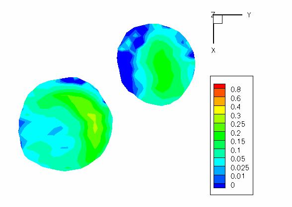
67 a) b) Figure 22. Comparison of axial velocity (m/s) for Model B at CC 2 at t 9 between a) the CFD calculations and b) the PCMR measurements. a) b) Figure 23. Comparison of axial velocity (m/s) for Model B at BI 1 at t 16 between a) the CFD calculations and b) the PCMR measurements. 51

68 a) b) c) d) Figure 24. PCMR data from Subject B at BI 1 for a) t 1 and b) t 5 and at BI 2 for c) t 1 and d) t Velocity profiles A survey of axial velocity distributions is made at the CC 1 slice location to better elucidate the importance of spatially variant velocity profiles. In Model A the axial velocity profiles at the common carotid inlet plane are skewed, and the location of the velocity peak shifts during the pulse cycle. At t 1 and t 2, the axial velocity profiles skew towards the position denoted by, roughly the rightanterior corner (Figure 25, Figure 27). At t 3 -t 6 the skewed velocity profile shifts clockwise towards the outer internal carotid with maximum axial velocities greater than m/s. The velocity profile begins to migrate more centrally through t 7 -t 10. In t 11 -t 15 the profiles again skew towards the outer internal carotid, but the peak velocities (>.646 m/s) are smaller than those in t 3 -t 6. 52

69 In Model B the axial velocity profiles migrate (right-anterior) over t 2 -t 4, until a band of high velocities are formed along the right side of the common carotid inlet from t 5 -t 7 (Figure 26, Figure 28). During that same time period, negative axial velocities are seen along the left side. The band of high velocities shifts centrally and posteriorly during t 8 and t 9, to be followed by a strong right-side skew at t 10. Throughout the rest of the cycle, the velocity profiles, although not perfectly symmetric, are relatively centered. Figure 25. Skewing of the Model A velocity profile towards the internal carotid artery at t 1. Figure 26. Skewing of the Model B velocity profile towards the external carotid artery at t 3. 53

70 t 1 t 2 t 3 t 4 t 5 t 6 t 7 t 8 t 9 t 10 t 11 t 12 t 13 t 14 t 15 Figure 27. Axial velocity contours of the Model A inlet plane at t 1 -t 15. At each time point there are 25 contours scaled to the minimum and maximum velocity values at each time point. 54

71 t 1 t 2 t 3 t 4 t 5 t 6 t 7 t 8 t 9 t 10 t 11 t 12 t 13 t 14 t 15 t 16 t 17 t 18 t 19 Figure 28. Axial velocity contours of the Model B inlet plane at t 1 -t 19. At each time point there are 25 contours scaled to the minimum and maximum velocity values at each time point. 55

72 Negative axial velocity regions Negative axial velocity regions (where U z 0) are illustrated over time for both human-based models. For an understanding of the flow field, it is useful to look at the inlet axial flow profiles in conjunction with the vessel geometry for interpretation of NAVR. As reported in Wake et al., (2005), at all BI 1 time points for Model A, there exists a dynamic NAVR along the outer wall of the external carotid at the external carotidcommon carotid (EC-CC) junction (Figure 29). During the pulse cycle the NAVR extends across the sides of the common carotid and into the proximal carotid sinus and the bifurcation region of the internal carotid artery. In the more distal regions of the internal carotid the flow becomes primarily axial; therefore, negative axial velocities are not seen. The sides of the common carotid and the internal carotid experience transient negative axial velocities, indicating these are locations of oscillatory axial wall shear stress. The NAVR changes over time; thus, along its perimeter, axial velocities change direction over time (i.e., the area experiences oscillatory axial wall shear stress). The smallest NAVRs are observed at t 1 and t 2, both of which are during the systolic acceleration period. In 10 of 15 time points, the NAVR stretches from the external carotid artery across the right side wall of the bifurcation [i.e., where the internal carotid branches away from the common carotid axis (Figure 9a)]. One striking feature in Model A is that during the t 3 -t 15 time interval, there exists a consistent subregion of negative axial velocity extending into the external carotid from the EC-CC junction (Figure 30). Although the cross-sectional shape of the region 56

73 changes and the entire bulbous region has some movement axially and circumferentially, it is a predominant feature in the negative axial velocity plots. In Model B regions of negative axial velocity are present throughout most of the cardiac cycle (Figure 31). At all but four time points (t 1, t 5, t 10, t 17 ) there exist negative axial velocities in the carotid sinus. This internal carotid NAVR is primarily in the carotid sinus at the IC-CC junction and across the left side of the carotid bulb [i.e., where the internal carotid branches out from the angle of the common carotid (Figure 10b)]. There exists significant negative axial flow in the external carotid artery in all but five time points (t 1, t 5, t 8, t 10, t 17 ). Primarily the region resides in the EC-CC junction; however, in two time points (t 4 and t 9 ) the region extends through the external carotid artery. Dramatic NAVRs are seen at t 4 during systolic deceleration, but the largest occurs at t 9, at one of the lowest flow rates and the time point at which the peak axial inlet velocity is directly opposite of the external carotid (Figure 28). At t 6 and t 9, the zone of negative axial velocity encircles the bifurcation region and extends the length of the modeled common carotid. These two points are the time points which have the lowest flow rates for any time points with skewed inlet velocity profiles, thus indicating the synergistic influence of the velocity distribution and the flow rate on formation of transient recirculation regions. 57

74 t 1 t 2 t 3 t 4 t 5 t 6 t 7 t 8 t 9 t 10 t 11 t 12 t 13 t 14 t 15 Figure 29. Regions of negative axial flow (blue) of Model A at t 1 -t

75 Figure 30. Extent of negative axial flow subregion through the external carotid in Model A at t 1 -t 15 and the location of the contours in reference to the bifurcation. 59

76 Figure 31. Regions of negative axial flow (blue) of Model B at t 1 -t

77 Wall shear stress Axial wall shear stress (WSS) values were averaged over all times at which PCMR data were taken for Model A and Model B. In both models a large region of negative axial WSS extends from the EC-CC junction into the external carotid artery (Figure 32, Figure 33). In these figures, the negative WSS is plotted as a positive value. In Model A the low WSS region swaths across the sides of the bifurcation region, with a finger of the region crossing the right-side wall to the IC-CC junction (Figure 32a, Figure 32b). For Model B the low axial WSS region extends across the left-side wall (Figure 33d) to the IC-CC junction/base of the carotid sinus region (Figure 33c). In both models the saddle point of the bifurcation is an area of locally high WSS, and the internal carotid artery has a higher average WSS than the external carotid artery. In both models a low average WSS region is present on the side of the bifurcation from which the internal carotid bifurcates from the common carotid axis (Figure 32a, Figure 33d). a) b) c) d) Figure 32. Average axial wall shear stress for Model A. 61

78 a) b) c) d) Figure 33. Average axial wall shear stress for Model B. Irrespective of the details of WSS distribution, however, is the fact that in both subjects the region of the bifurcation itself is one of relatively low mean WSS, thus implying that this area is likely to be much more susceptible to atherosclerosis than is the proximal common carotid or the distal segments of the daughter branches Womersley model Using the systolic flow rate and the geometry of Model A, a Model W was produced with Womersley velocity distributions as boundary conditions. Comparing the simulations of Model A and Model W isolates the influence of boundary velocity distributions on the computational results. Since diastole (the majority of the pulse cycle) is not included in the simulation of Model W, average wall shear stress comparisons will not be made. 62

79 Comparison with PCMR data Qualitative comparison with PCMR data is only cursory, since by the nature of the Womersley velocity profiles they are symmetric. The average maximum axial velocity difference based on the PCMR data was 69% for BI 2. As mentioned in the PCMR time points at CC 1 and CC 2 do not correspond to the simulation time points discussed here, but the axial velocities for Model W are compared with the values from the subject-specific Model A. The average maximum axial velocity differences normalized by the Model A velocity values were 7% for CC 1, 26% for CC 2, and 10% for BI 2. The difference in maximum axial velocities between Model A and Model W at CC 2 is no doubt related to the vast differences in NAVRs reported in Velocity profiles By definition, the velocity profiles of Model W are symmetrical, but since the common carotid inlet plane of the simulation is not precisely circular the profiles are slightly offset (Figure 34). It is obvious that there are significant differences in the axial velocity distributions at the inlet. The consequences of these differences on the development of negative axial flow regions are discussed in t 1 t 2 t 3 t 4 t 5 Figure 34. Axial velocity distributions at CC 1 at t 1 -t 5 for Model A (top) and for Model W (bottom). 63

80 Negative axial velocity regions In the subject-specific Model A, the region of negative axial velocity is small during systolic acceleration (t 1 and t 2 ) (Figure 35). This region grows axially and extends across to the IC-CC junction outer wall through systolic deceleration (t 3 and t 4 ) until a second acceleration (t 5 ), which leaves limited negative axial velocity in the internal carotid. During the second acceleration (t 5 ) the NAVR encroaches on the center of the artery more so than the NAVR developed during the systolic acceleration (t 2 ) (Figure 36) however, the larger region appears during an acceleration phase of lower slope than the initial systolic acceleration (Figure 11), so the NAVR at t 5 is expected to be larger than the one in t 2. During systolic acceleration Model W shows a significant zone of negative axial velocities across the side wall of the internal carotid sinus (t 2 ), but during systolic deceleration (t 3 and t 4 ) the NAVR clears from the bifurcation to the proximal common carotid region (Figure 35). During the second acceleration (t 5 ), a more extensive recirculation region appears than that at t 2 (Figure 37). As mentioned for Model A, the rate of acceleration likely influences the relative amount of reverse axial velocity. The development of an NAVR in Model W during systolic acceleration (t 2 ), then disappearance of the region during systolic deceleration (t 3 and t 4 ) is surprising and counterintuitive to the fluid dynamics concept of adverse pressure gradients in flow deceleration and warrants consideration of the geometry. In Model W at t 2 the axial profile is centered and sharply parabolic (Figure 38c), thus the high momentum fluid is in the center of the common carotid, and it consequently impinges upon the left side of the apex creating a recirculation region in the IC-CC junction (Figure 38d). Conversely, the 64

81 inlet axial velocity profile of Model A at t 2 is skewed towards the internal carotid artery (Figure 38a), and the concentration of high velocities along that wall may decrease any locally negative flow (Figure 38b) that would be prone to appear due to the sudden expansion at the bifurcation region and due in particular to the angle at which the internal carotid departs from the common carotid. At t 3 and t 4, the velocity profile in Model W flattens as compared to systolic distributions (Figure 39c, Figure 40c); therefore, the high momentum axial flow is more evenly distributed as it impinges upon the bifurcation point possibly inhibiting the development of an NAVR (Figure 39d, Figure 40d). At time points t 1 and t 5 the maximum axial velocity at CC 1 is greater in Model A than in Model W; however, at time points t 2 -t 4 the maximum axial velocity is greater in Model W. This may contribute to the differences in the NAVRs during the t 2 -t 4 time points. At t 5 the recirculation region in Model W extends across the side of the bifurcation into the IC-CC junction, whereas in Model A, the recirculation region is predominantly in the external carotid artery and the EC-CC junction of the bifurcation region (Figure 35). Most likely, the root of this discrepancy lies in the velocity distributions across the common carotid inlet. In Model A, the high velocities are skewed towards the internal carotid side (Figure 41a), minimizing the recirculation region (Figure 41b). As discussed for t 2, during the secondary flow acceleration (t 5 ), the Womersley velocity profiles become more sharply parabolic (Figure 41c) and impinge on the left side of the bifurcation apex, resulting in a recirculation region along the bifurcation side-wall from which the internal carotid branches (Figure 41d). 65

82 t 1 t 2 t 3 t 4 t 5 Figure 35. Negative axial velocity regions t 1 -t 5, for Model A (top), and for Model W (bottom). a) b) Figure 36. Extent of NAVR at a) t 2 and b) t 5 of Model A. a) b) Figure 37. Extent of recirculation region at a) t 2 and b) t 5 of Model W. 66

83 a) b) c) Figure 38. At t 2 a) subject-specific inlet axial velocity profile b) areas of negative axial flow in Model A, c) Womersley inlet axial velocity profile, d) areas of negative axial flow Model W. d) a) b) c) d) Figure 39. At t 3 a) subject-specific inlet axial velocity profile b) areas of negative axial flow in Model A, c) Womersley inlet axial velocity profile, d) areas of negative axial flow in Model W. 67

84 a) b) c) d) Figure 40. At t 4 a) subject-specific inlet axial velocity profile b) areas of negative axial flow in Model A, c) Womersley inlet axial velocity profile, d) areas of negative axial flow in Model W. a) b) c) d) Figure 41. At t 5 a) subject-specific inlet axial velocity profile b) areas of negative axial flow in Model A, c) Womersley inlet axial velocity profile, d) areas of negative axial flow in Model W. 68

85 4. Discussion and Conclusions Plaque location in the carotid artery bifurcation has been correlated with local fluid flow phenomena: flow separation, secondary flow, low wall shear stress, and oscillatory wall shear stress (Zarins et al., 1983, Ku et al., 1985). Subsequent experimental and numerical studies have attempted to refine or to refute this correlation by manipulating various parameters (e.g., fluid properties, wall properties, boundary conditions). Researchers have even qualified this correlation by asserting that although there might be neighborhoods (e.g., the carotid sinus and the internal carotid artery) in which the relationship between low and oscillating wall shear stress and plaque location hold, there is a possibility that no such simple relationship between local hemodynamics and wall thickness exists (Steinman et al., 2002). The results presented in this study seek to emphasize the importance of using patient-specific information--geometry and velocity distributions--when modeling the carotid artery and when analyzing hemodynamics in the context of atherogenesis and atherosclerotic development. As described earlier, discussion of the results of this study focuses on two flow field characteristics that have been reported to be related to atherosclerosis in human carotid arteries: wall shear stress (WSS) and negative axial velocity regions (NAVR). The latter is an indication of regions of transient flow separation and reversal and hence is related to changes in direction of WSS and to particle residence time. At first glance Model A and Model B demonstrate inter-patient variability in geometry, flow waveform, 69

86 and time-varying velocity profiles; however, certain trends associated with velocity profile skewing (e.g., average axial WSS and NAVR) are similar between the models. Therefore, as well as emphasizing the differences between models, it is useful to highlight any trends which transcend these differences. In this study both subjectspecific models exhibit NAVR, low average WSS, and secondary flow in the external carotid and along the side walls of the bifurcation. Comparing NAVR in Model A and Model W isolates the effects of inlet velocity boundary conditions on this flow phenomenon in individual human carotid models. This study demonstrates the influence of inlet velocity profiles on NAVR throughout the bifurcation regions, highlights the influence of the skewed velocity profiles on near wall negative axial flow in the daughter branches, and emphasizes the importance of patient-specific modeling in WSS calculations Findings There are many studies implicating hemodynamics and local flow patterns on the formation and progression of atherosclerotic plaques; particularly, carotid bifurcation studies have correlated maximum intimal thickness with separation regions and low WSS at the outer wall of the carotid sinus (Zarins et al., 1983). This study focuses on NAVR and low time-averaged WSS regions because of their relevance to atherogenesis. Transient separation regions are implicated in atherosclerosis development 1) by creating a flow environment which allows particles in the flow a longer time for local mass transport into the vessel wall (Giddens and Ku, 1987), and 2) by creating flow conditions which affect endothelial layer permeability (Rappitsch and Perktold, 1996). Many 70

87 studies connect low and oscillatory wall shear stress zones to atherosclerotic lesion locations (e.g., Zarins et al., 1983; Ku et al., 1985; He and Ku, 1996), whereas high wall shear stress regions, especially the bifurcation apex, show minimal thickening (Zarins et al., 1983). It is demonstrated in this work that subject-specific velocity profiles in the common carotid artery proximal to the bifurcation are major factors influencing local flow environments that have been shown to favor atherogenesis Inlet velocity distributions affect negative axial flow patterns By in large, previous numerical studies of subject-specific time-varying flow through a subject-specific carotid artery bifurcation impose an idealized Womersley velocity distribution at the inlet of the bifurcation, and do so in one of two ways: 1) decomposing a measured flow waveform, from US data or from integrating MR velocity data, into the corresponding Womersley velocity profiles (e.g., Younis et al., 2004; Glor et al., 2003, Steinman et al., 2002), or 2) imposing the measured flow waveform as bulk flow at the inlet of a long entrance region to the carotid bifurcation, allowing the development of fully-developed velocity profiles before the bifurcation is reached. One study sought to quantify WSS and oscillatory shear index (OSI) differences between models with Womersley inlet conditions and with asymmetric inlet conditions introduced by a helical entrance region (Moyle et al., 2005). Using a patch test comparison (where parameter values were averaged over small surface regions to facilitate comparison) of WSS and OSI for different entrance length geometries and for different measurements/reconstructions of the same subject, Moyle et al., (2005) concluded that differences in these time-averaged parameters due to the degree of asymmetry of the inlet 71

88 velocity profiles were less than the differences arising from intra-patient variability due to geometry reconstruction reported in Thomas et al., (2003). Thomas et al., (2003) attribute the majority of the intra-patient variability in the wall shear stress and wall shear stress derived parameters to the lumen segmentation and reconstruction steps (and, implicitly, data resolution), emphasizing the importance of a reliable, consistent method of constructing the model. Comparison of the regions where the axial velocity is negative between Model A and Model W demonstrates that with identical geometry and flow waveforms, the imposed velocity profiles at the inlet strongly influence the location, and even existence of, the NAVR (Figure 35). Subject geometry, flow waveform, and inlet velocity profiles synergistically affect the locations of negative axial velocity in the carotid bifurcation. The NAVR in subject-specific Model A develops over systolic deceleration, and a significant transient separation region remains at the accelerating time step, t 5. In time steps t 1 -t 4 the separation region develops as would be expected due to the adverse pressure gradient created by decelerating flow: the NAVR is small during acceleration and grows during systolic deceleration. At time point t 5 there is a secondary inlet flow acceleration which would not be expected to produce an adverse pressure gradient and, consequently, negative velocities near the wall; however, the inlet velocity profile of Model A is strongly skewed towards the internal carotid artery (Figure 34), encouraging the formation of an NAVR in the external carotid artery, and inhibiting development of such a zone in the internal carotid artery. In contrast a large NAVR develops in Model W across the side wall of the internal carotid sinus during systolic acceleration, and this region all but disappears during systolic deceleration (Figure 35). During the second 72

89 acceleration at time point t 5, a more extensive separation region appears. In Model W the parabolic profiles impinge on the left side of the bifurcation apex, causing reversal of velocities along the side wall from which the internal carotid branches. This suggests that this velocity distribution in combination with the geometry influences the negative axial velocity region development more than the flow waveform. The slower acceleration rate at t 5 than at t 2 (Figure 11) likely contributes to creating a larger zone of negative axial velocity. Thus, there are significant temporal and spatial differences in negative axial flow region development, and hence in near-wall flow behavior, between models with idealized (Model W) and subject-specific (Model A) velocity boundary conditions. Further, Figure 27 and Figure 28 demonstrate the inter-patient variability of the timevarying inlet velocity profile. It is therefore likely that the asymmetry imposed by helical entrance flow regions (Moyle et al., 2005) does not adequately represent the time-varying inlet velocity distributions in humans; and their conclusion that inlet velocity profiles have little effect on the bifurcation flow field may not be generally applicable Inlet velocity distributions affect negative axial flow location It is widely reported that local geometry differences between subjects impact flow patterns in models (Moore et al., 1998; Milner et al., 1998; Perktold et al., 1994). Moore et al., (1999b) reported that numerical models with geometric or flow rate differences predicted similar gross trends (e.g., low WSS region location), and both geometry and flow rate were found to quantitatively affect the amount of flow reversal and the 73

90 existence of flow reversal. The findings in confirm that the velocity boundary conditions also affect the NAVR location. In this study it was found that the daughter artery towards which the inlet axial velocity profiles are skewed has less extensive NAVR (spatially and temporally) than the other daughter. In Model A the inlet velocity profile is predominantly skewed towards the internal carotid (Figure 27), and the negative axial flow region lies primarily in the external carotid artery with some negative axial flow along the side wall of the bifurcation from whence the internal carotid artery bifurcates (Figure 29). In Model B, the velocity profile is skewed towards the right side (Figure 28), but not strongly skewed towards one or the other daughter artery. The negative axial flow region in Model B varies over the pulse cycle (Figure 31), but there is not substantially greater negative axial flow region in either daughter artery. The largest NAVR in the external carotid of Model B exists at time point t 9, the time point at which the inlet velocity profile is most strongly skewed away from the external carotid artery. Further, as discussed in the comparison of negative axial flow regions between Model A and Model W reinforces the connection between inlet axial velocity profiles and negative axial flow regions. Typically, negative axial flow regions are reported in the internal carotid (e.g. Balasubramanian, 1980); however, a few studies mention some secondary recirculation regions in the external carotid (e.g. Perktold and Rappitsch, 1995; Steinman et al., 2002). Both of the subject-specific models considered in this study have negative axial velocity regions in the external carotid, apparently as a consequence of the geometry and the inlet velocity boundary conditions. 74

91 Location of lowest axial wall shear stress is subject-specific Typically, the area of lowest WSS is found in the IC-CC junction or the internal carotid bulb, both in studies of the averaged human carotid bifurcation model (e.g., Balasubramanian, 1980) and of individual human carotid bifurcations (e.g., Younis et al., 2004). Milner et al., (1998), reported that the carotid bulb had the lowest average WSS in all models studied, but the pattern of the low WSS region was found to vary with flow rate, implicating a synergistic effect of geometry and flow waveform. Moore et al. (1999b) also found that flow rate and geometry changes quantitatively affect the magnitude of WSS. Previous studies in models of the carotid bifurcation identify the outer walls of the carotid sinus as the region with the lowest mean WSS. For both subject-specific Model A and Model B in this study the lowest average WSS region extends from the external carotid artery along the side of the bifurcation region (Figure 32 and Figure 33). Specifically, there is a finger of low average WSS extending to the internal carotid along the side from which the internal carotid bifurcates from the common carotid. Not surprisingly, there exists an area of high average WSS at the apex of the bifurcation of both models. However, there is generally lower WSS in the bifurcation itself than in the proximal common carotid or in the distal daughter branches, consistent with clinical observations that the bifurcation is a preferred site for atherogenesis. These results point to the need for caution in generalizing results from an average, planar model of the carotid artery to predictions in individual subjects. Admittedly, n=2 is a small sample size. However, the current study suggests not only might patient-specific geometry and flow rate affect the patterns of low WSS (Milner et al., 1998), but the inlet 75

92 velocity distribution also influences the position and extent of low WSS regions. It should be noted that the velocity boundary conditions of Model A and Model B are subject-specific, whereas earlier studies reporting lowest average WSS in the internal carotid imposed developed flow as inlet conditions Limitations Two of the greatest limitations of this study are due to data acquisition and to model simplifications. The hesitancy to declare CFD simulation as the long-sought gold-standard in hemodynamics is rooted in the knowledge that the integrity of a model is limited by its boundary conditions (both geometry and time-varying inlet/outlet conditions). Additionally, the rigid wall assumption is thought to influence the current study to a degree MRI A simulation is only as good as its boundary conditions. Sources of error introduction via data acquisition considered here are registration challenges, flow split imposition, and velocity measurement Registration of PCMR to MR data As mentioned before, some error is introduced through registration of the PCMR data to the corresponding location in the computational model. In these models, the axis of the geometry scan was defined as normal to the PCMR data planes. In Model A, the geometry scan, the CC 1 PCMR scan, and the CC 2 PCMR scan were conducted with near- 76

93 identical rotation matrices (i.e., the orientation of the scans relative to the magnet were essentially the same), but the PCMR scan at BI 2 was not in the same orientation. The non-alignment of the BI 2 scan with the two proximal PCMR measurements and the geometry scan likely contributes to the average maximum axial velocity differences seen at BI 2 (Table 8). In Model B all PCMR data slices were obtained in the same orientation, but the geometry was not aligned in the same axial direction. This influences the average maximum axial velocity difference at the two PCMR locations distal of the bifurcation (Table 9). It is important to note the CC 1 PCMR plane is not normal to the Model B common carotid axis (Figure 10a). The boundary conditions at the inlet plane were not applied in the same direction relative to the common carotid axis as they were measured (the common carotid axis is approximately normal to the PCMR measurement plane at the inlet); therefore, the direction of the total velocity in the real vessel is probably more aligned in the axial direction of the common carotid artery than is reflected in the simulation. With this orientation of the flow with the common carotid artery, less secondary flow is expected in the real artery than is demonstrated in the model. Further, if a single velocity component is measured at a single PCMR slice location distal of the bifurcation, there is a distinct probability that the axial direction of at least one daughter branch will be oblique to the measurement plane. Hence, the outflow magnitude will be under predicted for at least one daughter branch, possibly affecting flow splits between daughter branches and comparisons of axial velocity. 77

94 Flow split estimation The importance of accurate flow division is reaffirmed in both experimental and numerical studies. In steady flow for a given geometry, fluid flow phenomena are influenced more by the outlet flow rate ratio than by the Reynolds number (Zarins et al., 1983). Interpreting pulsatile flow results, Younis et al., (2002) suggest that WSS values in the external carotid artery were erroneously large because there was overestimated flow through the external carotid artery; coincidentally, they saw flow separation primarily at the IC-CC junction. As discussed in 3.1.1, the determination of velocities from PCMR data may have resulted in an estimate of a higher proportion of flow through the internal carotid of the models than actually existed in the subjects. In both Model A and Model B, regions of negative axial velocity are seen in the external carotid artery over a majority of the pulse cycle. This could be due to the low percentage of flow through the external carotid artery as compared to other studies (e.g., Ku, 1983). Intuitively, increased flow division to the internal carotid artery could create or exacerbate separation regions in the external carotid artery and could inhibit or decrease separation regions in the internal carotid artery. This phenomenon was reported by Balasubramanian (1980) and is demonstrated by the simulations in 2.3.1, namely, that for a constant Reynolds number in a steady flow, the size of the separation region in the internal carotid artery grows as the percentage of flow through the external carotid artery increases. Applying this principle to the other daughter artery, as flow through the internal carotid artery increases, separation regions along the EC-CC junction outer wall would be expected to increase. 78

95 Velocity measurement Botnar et al., (2000), found that peak axial velocities vary less than 10% between in vitro PCMR measurements and CFD calculations for pulsatile flow in a planar, compliant carotid bifurcation model, but for secondary flows, the difference is greater and is inversely related to vessel diameter. Zhao et al., (2002), also note the axial velocity uncertainty is on the order of 5% of the velocity encoded value, which in Model B corresponds to roughly 6.25 cm/s, with high velocity gradients generating more measurement inaccuracies. The differences between average maximum axial velocities as measured by PCMR and calculated by CFD at the BI 1 (26%) and BI 2 (27%) planes are both greater than the uncertainty reported by Zhao et al., (2002), implicating other sources of error, possibly registration as mentioned in Maximum axial velocity differences calculated for post-bifurcation PCMR measurement planes Models A and B are significantly larger than those reported in Botnar et al., (2002). It must be emphasized that those simulations were conducted for an in vitro, planar, compliant bifurcation model, thus representing the lower bound of error; Model A and Model B are non-planar, rigid geometries developed from in vivo measurements Modeling assumptions The results in this study are based on using only the measured axial component of velocity for the velocity boundary conditions. Although inclusion of accurate secondary velocities would create more physiologically faithful boundary conditions, Zhao et al., (2002), contend that the MR measured secondary velocity errors are high (30% in ICA 79

96 and 50% total at peak systole), and the secondary velocities are sufficiently smaller than the axial velocity that they do little to affect the total velocity. However, Zhao et al., (2002), examined a systolic-like waveform, and in Steinman et al., (2002) secondary velocities increased in diastole. Perktold and Rappitsch (1995) found that secondary velocities decrease in the compliant model. Thus, increased measurement time and the computational expense required to include all three components of velocities at the boundary locations might not be worthwhile at this stage, but should be considered in future modeling endeavors. The flow simulations reported here were conducted in rigid models, but real arteries are compliant; therefore, when interpreting simulation data an understanding of compliance effects is useful. Comparing compliant and rigid models demonstrated that differences in average wall shear stress and separation points in planar, averaged human carotid bifurcation models were not large (Anayiotos et al., 1994; Anayiotos, 1990), and differences in individual geometries were reported to influence recirculation regions and peak wall shear stress more than the inclusion of compliant wall modeling (Perktold et al., 1994); however, quantitative differences in flow phenomena are seen between compliant and rigid wall models (Perktold and Rappitsch, 1995). In the PCMR measurements of Subject B, there is observable expansion and translation of the artery over time; particularly at locations BI 1 and BI 2, the artery movement is seen in concert with lumen distortion of the neighboring vein (Figure 24). However, for the creation of the model, the MR data were obtained during diastole and the model was assumed rigid. In both subject-specific models the largest errors at BI 2 occur at peak systole and during early systolic deceleration. These measurements are consistent with the 80

97 observations of Perktold and Rappitsch (1995), who report that during systolic acceleration axial velocities are lower in compliant models than in rigid models. The greatest differences between PCMR and calculated maximum axial velocity occurred during systolic acceleration for both models at measurement plane BI 2. Based on experiments by Perktold and Rappitsch (1995) because of expansion during systolic acceleration, PCMR measured axial velocities are expected to be lower than those calculated in the rigid Model A and Model B; however, during deceleration, they should have closer agreement, since the geometries were constructed from images taken during diastole. It is expected that a compliant bifurcation would have larger side wall NAVR and less extensive negative flow regions at the IC-CC and EC-CC junctions than the simulation results (Perktold and Rappitsch, 1995). Inclusion of compliant walls would also be expected to increase the size of the low average WSS region along the side of the bifurcation from which the internal carotid artery splits from the common carotid. However, the NAVR in the external carotid arteries are substantial; and while they might recede in a compliant model, they are not expected to disappear. Reuderink (1991) reported smaller recirculation regions in a compliant model than in a rigid model and demonstrated smaller recirculation regions and lower WSS near peak systole in the compliant model than in the rigid model Conclusions In conclusion, this study has demonstrated several significant findings. The research underscores the difficulties and errors inherent in employing MR and PCMR 81

98 data to obtain accurate information from which to construct CFD models, even when using sophisticated segmentation techniques. Despite these limitations in methodology, the importance of imposing subject-specific inlet velocity boundary conditions when developing models for use in understanding clinically relevant flow parameters is clearly demonstrated. In the subject investigated here, imposing a Womersley flow as inlet boundary conditions does not give the same results for important flow variables such as WSS and NAVR. Additionally, the significant effects of non-planarity are demonstrated by comparison of the two subjects with previous simulations of a planar geometry. The study highlights the importance of the local geometry in the bifurcation itself, especially the location of the flow divider with respect to the branches and significantly with respect to the velocities impinging from the common carotid artery. Finally, at least under the assumptions and limitations of the simulations, the finding that there is significant NAVR in the external carotid branch in these two subjects was striking. It is known that plaques do develop in the external branch in some individuals, and the generalization that atherogenesis first occurs at the outer wall of the internal branch may not hold for all subjects. There are three natural extensions of this work: 1) to include vessel compliance in the flow model, 2) to measure and to incorporate all three velocity components as boundary conditions, 3) to increase the sample size of normal subjects, and 4) to extend this technique to modeling carotid arteries of patients with carotid plaque. 82

99 Appendix A: Phantom model details Comparison of in vitro experimental results of Balasubramanian (1980) to the computational results in this study is qualitatively favorable as discussed in It is important to note there is a significant difference in measurement resolution between the flow visualization and Laser Doppler Anemometer (LDA) data (Balasubramanian 1980) and the finite element results presented here. Figure A.1 shows the location of planes used for comparison of velocities between the in vitro results and the computational model results. For the computational model the ICA6 location was beyond the extent of the Sylgard model; rather, that location was in the exit length added to the computational model (Figure A.1.b). There is a discontinuity at the junction of the exit length and the computational model of the phantom. This discontinuity contributes to the differences between the in vitro results and the numerical results of the measured axial velocities at ICA6 (Figure 6). As demonstrated in Balasubramanian (1980), for a constant flow division the recirculation region in the IC-CC junction grows with increasing Reynolds number (Figure A.2). The velocity profiles at the internal carotid measurement planes agree well between the in vitro flow experiments and the CFD calculations both in the plane of bifurcation (Figure 6) and in the plane perpendicular to the plane of bifurcation (Figure A.3). For the computational results, the velocities in both figures are normalized by the average inlet axial velocity, and the distance is normalized by the local diameter. 83

100 ICA6 ICA5 ICA4 ICA3 ICA2 ICA1 CCA4 CCA3 CCA2 CCA1 a) b) Figure A.1. Location of comparison planes of a) the large-scale model of the averaged human carotid bifurcation (Balasubramanian, 1980) and b) the computational model of the Sylgard phantom. Along the common carotid, CC1 corresponds with CCA1, CC2 corresponds with CCA2, CC3 corresponds with CCA3, and CC4 corresponds with CCA4. Along the internal carotid x i =0.90 corresponds with ICA1, x i =1.35 corresponds with ICA2, x i =1.81 corresponds with ICA3, x i =2.26 corresponds with ICA4, x i =2.73 corresponds with ICA5, and x i =3.2 corresponds with ICA6. 84

101 a) b) c) Figure A.2. For a constant flow ratio, IC:EC=70:30, the CC-IC recirculation region (blue) grows as the Reynolds number increases: a) RE=400, b) RE=800, c) RE=1200. a) b) Figure A.3. Velocity profiles in the plane perpendicular to the plane of bifurcation for RE=400, IC:EC=70:30 a) from Balasubramanian (1980), b) from computational results. 85