Modeling and Characterization of Neural Gain Control. Odelia Schwartz. A dissertation submitted in partial fulfillment

Transcription

1 Modeling and Characterization of Neural Gain Control by Odelia Schwartz A dissertation submitted in partial fulfillment of the requirements for the degree of Doctor of Philosophy Center for Neural Science New York University September 22 Eero P. Simoncelli

2 c Odelia Schwartz All Rights Reserved, 22

3 ACKNOWLEDGMENTS I am most grateful to my advisor, Eero Simoncelli, for all the time, support, and enthusiasm he has given throughout the course of this research; and for his many inspiring ideas and computational insights. I have learned so much from him. I am very thankful to my other committee members, Mal Semple and Tony Movshon, for discussions and advice; and to my examining committee, Carlos Brody and Dan Tranchina, for suggestions and comments about the manuscript. I thank everyone in the Simoncelli lab for their support over the years. This work has been enriched through discussions with Javier Portilla, Jonathan Pillow, Jesus Malo, and Liam Paninski. I am grateful to James Cavanaugh, Wyeth Bair, and Nicole Rust in the Movshon lab for sharing their data and for discussions. Many thanks to EJ Chichilnisky for his experimental collaboration and suggestions on the spike-triggered covariance work. Thanks also to Divya Chander for data collection. Special thanks to John Harris, my former MS advisor; he encouraged my interest in computational sensory processing, and has often given me advice throughout the years. I am very grateful to Sam Feldman and Stu Greenstein for their help and dedication during my time at the Center for Neural Science. Thanks to friends and classmates for their help, and for making my time more enjoyable. I thank my parents for their constant love and support. iii

4 And to Shlomi, my husband and best friend, thank you for going through this with me. Contributions include but are not limited to help with figures, love, encouragement, delicious meals, and sense of humor. Funding during my time at the Center was provided by the Sloan-Swartz foundation and the National Eye Institute (NEI). iv

5 ABSTRACT Sensory neurons often exhibit striking nonlinear behaviors that are not adequately described by a linear receptive field representation. In the first part of the work, we suggest that these nonlinearities arise because sensory systems are designed to efficiently represent environmental information. We describe a form of nonlinear decomposition (specifically, divisive gain control) that is well-suited for efficient encoding of natural signals. We show that this decomposition, with parameters optimized for the statistics of a generic ensemble of natural images or sounds, can account for some nonlinear response properties of typical neurons in both vision (area V1) and audition (auditory nerve). This work provides theoretical justification to neural models of gain control, and explains how one might choose the parameters of the model based on efficient coding considerations. In the second part of the work, we describe a methodology for characterizing this class of nonlinear sensory models. The characterization is based on a white noise analysis, in which a set of random stimuli are presented to a neuron and the spike-triggered ensemble (specifically, the spike-triggered covariance) is analyzed. We demonstrate the applicability of the technique to retinal ganglion cell data in monkey and salamander. The concept of gain control appears to be ubiquitous, occurring throughout the nervous system. So the computational tools we develop here may potentially have more widespread applicability. v

6 TABLE OF CONTENTS ACKNOWLEDGMENTS iii ABSTRACT v LIST OF FIGURES ix 1 INTRODUCTION Theory Driven Sensory Neural Models History and Outline Information Theory The Efficient Coding Hypothesis Biological Relevancy of Efficient Coding Alternative Coding hypothesis: Sparse Coding Testing the Statistical Hypotheses Open Questions in Theory Driven Models Physiology Driven Sensory Neural Models Physiological Nonlinearities in Sensory Neurons Nonlinear Models Stemming from Physiological Observations Open Questions in Physiology Driven Models vi

7 1.3 Spike-triggered (White Noise) Characterizations Open Questions in Spike-triggered (White Noise) Characterizations The Current Work NATURAL SIGNAL STATISTICS Methods Natural Signal Statistics Through One Linear Filter Statistical Dependency Through a Pair of Linear Filters Modeling the Statistical Dependency Reducing the Statistical Dependency: Divisive normalization Testing the Model Empirically Discussion NATURAL SIGNAL STATISTICS MODEL VS. PHYSIOLOGY Primary Visual Cortex Methods Mapping out the Receptive Field Comparison to Physiology Inside the Classical Receptive Field Mapping the Region Outside the Classical Receptive Field Comparison to Physiology Outside the Classical Receptive Field Cell and Model Variations in area V Auditory Nerve Methods vii

8 3.2.2 Comparison to Auditory Nerve Physiology Cell and Model Variations Discussion SPIKE-TRIGGERED COVARIANCE CHARACTERIZATION Characterizing a Neuron with Gain Control Estimating Excitatory Kernel with STA Estimating Suppressive Subspace with STC Estimating Suppressive Subspace in Simulation Estimating Suppressive Subspace in Retinal Ganglion Cells Fitting Specific Model Within Reduced Subspace Correcting for Bias in Kernel Estimates and Explaining Changes in the STA Extensions Discussion Proofs GENERAL DISCUSSION 173 BIBLIOGRAPHY 18 viii

9 LIST OF FIGURES 1.1 Natural image and sound vs. random white noise Restriction of decomposition of natural signals into linear components Behavior of Naka-Rushton equation Illustration of spike-triggered analysis Representative linear visual and auditory filters Responses of a linear filter to example image and sound Distribution of responses of linear filter to example image and sound Responses of pairs of linear filters to example image and sound Joint statistics of typical natural images and sounds as seen through two linear filters Joint statistics of different images and sounds through two linear filters Set of filters obtained from Bell and Sejnowski s ICA procedure Dependency for pair of filters retrieved from ICA analysis Image and sound statistics for different filter pairs Image and sound statistics for different signals and filter pairs Two dimensional joint conditional histogram of filter response versus its model prediction ix

10 2.12 Two dimensional joint conditional histogram following divisive normalization Additional examples of two dimensional joint conditional histograms following divisive normalization One dimensional marginal histograms following divisive normalization Additional examples of marginal histograms following divisive normalization Generic normalization model for vision and audition Phenomenological neural model for vision and audition Neighborhood for vision optimization Ensemble of images Mapping out the classical receptive field Cross-orientation suppression in area V Orientation masking in area V1 inside the classical receptive field Contrast invariance of orientation tuning in area V Examination of model components of orientation tuning as a function of contrast in area V Mapping out the surround annulus inner diameter Contrast response curves for parallel versus orthogonal surround masks in area V Surround suppression as a function of orientation for optimal center stimulus in area V Dependence of surround suppression on center orientation in area V1 98 x

11 3.13 Model dependence of surround suppression for different separations of center and surround with optimal center stimulus Model dependence of surround suppression for different separations of center and surround with non-optimal center stimulus Response as a function of surround inner diameter in area V Nonlinear changes in tuning curves as a function of stimulus diameter for different input levels in area V Distribution of physiological recordings from different cells, for parallel versus orthogonal surround in area V Distribution of model simulations with weights computed for different natural images, for parallel versus orthogonal surround Distribution of model simulations with weights computed for different natural images, for parallel versus orthogonal surround (part 2) Neighborhood for auditory optimization Suppression of responses to optimal stimuli by masking stimuli in auditory nerve fiber Model response for masking stimuli that exerts both excitation and suppression Nonlinear changes in frequency tuning curves as a function of sound pressure level in auditory nerve fiber Examination of model components for nonlinear changes in frequency tuning curves as a function of sound pressure level Nonlinear changes in frequency tuning curves as a function of sound pressure level for low center frequency in auditory nerve fiber xi

12 4.1 Geometric depiction of spike-triggered averaging Geometric depiction of spike-triggered covariance analysis of suppressive axes Estimation of excitatory and suppressive kernels from a simulated model Estimation of kernels for a salamander ganglion cell Nested Monte Carlo hypothesis testing of number of suppressive axes in salamander ganglion cell data Examples of estimated kernels in salamander ganglion cells Examples of estimated kernels in monkey ganglion cells Scatter plots of stimuli projected onto estimated kernels for salamander ganglion cell Scatter plots of stimuli projected onto estimated kernels for monkey ganglion cells Division versus subtraction in salamander retinal ganglion cells Division versus subtraction in monkey retinal ganglion cells Change in STA kernels for different contrasts in salamander retinal ganglion cell Demonstration of estimator bias ML retrieved model for salamander cell ML estimated model producing changes in the STA as a function of contrast for salamander retinal ganglion cell Data and ML retrieved model changes in the STA for different contrasts in salamander retinal ganglion cells xii

13 4.17 Data and ML retrieved model changes in the STA for different contrasts in monkey ganglion cells Facilitation in monkey retinal ganglion cell Estimated kernels in V1 direction selective complex cell Estimation error as a function of sample size xiii

14 CHAPTER 1 INTRODUCTION We interact with stimuli in the natural world through the senses. Locating predator or prey in the jungle, or recognizing a face in a crowded subway we are constantly making sense of a complex environment. This puts to work a plethora of neurons that process the information at various stages, resulting in perception, and ultimately, in action and storage of memory. Within this very intricate system, this thesis aims to understand: why do neurons form the particular representations that they do? And how can we characterize sensory neural representations? Specifically, we focus on neurons at relatively early stages of processing, including the retina, the primary visual cortex (area V1), and the peripheral auditory system. To answer these types of questions, we have studied neural behaviors at the signal processing, phenomenological level. This approach typically does not reveal a particular physiological mechanism; but will often initiate complementary exploration of the processes of biochemistry, spike generation, synaptic mechanisms, circuitry, and so on. Images in the world are initially represented in a rather pixelated form, by the 1

15 light intensities that impinge upon the photoreceptor array. We are interested in the types of representations that neurons form of their input stimuli along the sensory pathway. Perhaps the simplest representation we tend to think about, and which physiologists often measure, are receptive fields (or filters) over localized regions in space and time. For example, Hubel and Wiesel swept bars across the receptive spatial regions of neurons in V1, and found that neurons were selective (and responded with a higher firing rate) to particular orientations [67]. In this way, one can map out a receptive field of a neuron, which represents, roughly, what stimuli the neuron responds to best. If a neuron were truly linear, then one could make a prediction about its response to any given stimulus, just by knowing its receptive field. This would simply be the projection of the stimulus onto the receptive field (of course, in practice, even if one attempts to describe only the mean firing rate of the neuron, one must at least include a rectifying nonlinearity). However, receptive field characterizations are often not sufficient to describe the complexities of sensory neural behaviors. For example, in primary visual cortex, the response of a neuron to the optimal stimulus (e.g., that which is exactly equal to the receptive field) can be modulated by superimposing a second stimulus that by itself elicits no response at all in the neuron. This is a nonlinear behavior, suggesting that the representation is governed by other stimulus directions, and not just that given by the linear receptive field. These and other observations have suggested that a model of linear neural representation is too simplistic. In this chapter we provide a literature review, that feeds on both theoretical and experimental work in the field. We first describe neural models that have been 2

16 derived purely from theoretical principles. We show that such models have been fruitful in explaining some basic aspects of sensory representation, particularly regarding linear receptive field properties measured physiologically. But examination of physiological data reveal that sensory neurons are highly nonlinear. Indeed, physiology driven neural models have been developed that can account for some of these nonlinearities (specifically, gain control models). Finally, we describe how one can characterize individual neurons, assuming a particular form of underlying model. Specifically, spike-triggered approaches have been successful in characterizing some response properties of sensory neurons, but have not proceeded to characterize gain control models. This lays out the groundwork and motivation for the remaining chapters of the thesis. 1.1 Theory Driven Sensory Neural Models History and Outline Many factors are likely to shape sensory processing, including: the particular tasks an animal must perform; the capabilities and limitations of neurons; and the structure of the sensory stimuli that neurons receive. Here, we limit the discussion to how the structure of sensory stimuli in the world effect neural processing. This is an area that has been widely studied, and in which specific hypotheses about neural processing have been formulated. Stimuli in our sensory environment are highly structured and non random (Figure 1.1). Of all the possible could-be images and sounds, we are exposed to only a small portion in our particular environment. Since some stimuli are more likely to 3

17 Figure 1.1: Natural image and sound vs. random white noise 4

18 occur than others, it seems reasonable that our sensory systems are most suited to process those stimuli that occur most frequently. Early notions about sensory stimuli and the mind may actually be traced back to Greek philosophy. Aristotle held that the mind was a tabula rasa or clean slate; and that this slate is only filled with knowledge after sense experience. More modern versions of this idea were influenced by landmark scientific advances: with the discovery of nerve cells; with evolution emerging in the mid nineteenth century; and Shannon s information theory in the mid twentieth century. It has been widely assumed that neurons in sensory areas of the brain are adapted, through processes of evolution and development, to the signals to which they are exposed 1 [85, 16, 161, 39, 11, 16]. Information theory provided a quantitative framework for converting these ideas into a more concrete hypothesis about neural processing. Attneave and Barlow hypothesized that the brain develops in response to the statistical properties of the natural stimuli it is exposed to and does so in a manner that is efficient (henceforth, will be referred to as efficient coding hypothesis). We will define efficient shortly, from the point of view of information theory. In the past decade or so, the efficient coding hypothesis has spurred renewed interest (see also review article [14]). This is due to recent computational advances in the statistical analysis of natural images and sounds. In addition, advances in experimental techniques are beginning to pave the way towards more direct routes for testing this hypothesis. 1 Adaptation over shorter time scales to environmental signals is also assumed to effect neural processing, see [17, 165, 49]. 5

19 In the following sections, we first describe the computational building blocks of information theory, and how they relate to forming an efficient representation. We then explain how these ideas have led to the efficient coding hypothesis. Subsequently, we describe an additional hypothesis that has emerged, sparse coding. Finally, we describe computational and experimental work that have been aimed at testing these hypotheses Information Theory Information theory was developed to help engineers in the transmission of signals over communication devices [132, 133]. The theory is deeply rooted mathematically, and has been applied to numerous other areas that require efficient processing of signals. Hence, the theory may potentially be relevant to neural computation. Here we introduce only the most basic concepts necessary for our discussion (see [133, 38] for a more complete and detailed description). Consider an ensemble of signals that contain symbols, such as letters of the English alphabet, light intensity values in images, sound pressure levels in sounds, and so on. We assume that these input signals are passed through channels. The outputs are typically constrained by the architecture of the channels. A goal of information theory is that the output signals through the channels form a more efficient representation of the input. To achieve this goal, Shannon introduced (among other terms) redundancy, entropy, and mutual information. Related ideas were later developed in the framework of minimum description length, with the goal of creating a compact and efficient representation of observed signals, from which the original observed signals can be regenerated [148, 118, 17]. 6

20 Additional work has also focused on efficient coding using rate-distortion criteria (see [38]), and extraction of the most relevant information from a signal, while forming an efficient representation [151]. These directions are beyond the scope of this thesis. Redundancy Signals are considered inefficient in their representation, if they are redundant. There are two forms of redundancy that can occur in signals: some symbols occur more frequently than others (in the English language a occurs more often than q ); and, some symbols co-occur more frequently than others, i.e., they are not independent (letters sh are more likely to appear together than sd ). A more efficient representation is formed by reducing the redundancies in the signal ensemble. It is important to note that efficiency is only meaningful for a particular stimulus ensemble, and what is efficient for one ensemble is not necessarily efficient for another. Entropy and Mutual Information To quantify the notion of redundancy reduction, we define some basic terms from information theory. We denote X the set of input signals and Y the set of output signals (through one or more channels). The entropy of the output is given by: H(Y ) = y P (y) log 2 P (y) (1.1) 7

21 where P ( ) is the probability distribution. Entropy is a measure of how informative signals in the ensemble are on average. The information for each signal y is given by log 2 P (y) and multiplied by the probability of occurrence of the signal. Entropy is always positive, and equal to zero if and only if the outcome is certain; that is, P (y) is for all but one of the signals y which occurs with probability 1. The log2 indicates that information is expressed in units of bits. Stated in coding terms, entropy is the average number of bits needed to represent values drawn from a distribution. We first assume that the output is deterministically determined from the input. Then the representation is made less redundant and more efficient by maximizing the entropy of the output signals. So in the resulting representation the output is on average less predictable, and carries more information. But many systems, including neurons, are not deterministic: if a neuron is stimulated repeatedly with the same stimulus, the response is variable (we ll denote this variability by the term noise ). We d like to achieve maximal entropy of the output that s only due to the input. To do so, we need a measure for the amount of information between the output and the input. We take a small detour to achieve this goal. First, we define the Kullback-Leibler (KL) divergence (also called relative entropy), which is a measure of similarity between any two probability distributions, P and Q: D(P Q) = k P (k)log 2 P (k) Q(k) (1.2) KL is always positive and equal to zero if and only if Q and P are equal. This measure can also be interpreted as the average number of bits lost encoding samples 8

22 of P assuming Q as a model for the distribution. We define the mutual information I(X, Y ) as a special case of KL, in which: P = P (x, y) and Q = P (x) P (y): I(X, Y ) = D(P (x, y) P (x) P (y)) = x,y P (x, y) log 2 P (x, y) P (x) P (y) (1.3) The mutual information is equal to zero if and only if P (x, y) = P (x) P (y); that is, by definition, if and only if the input and output are independent. We now express the mutual information in terms of entropy. Using Bayes rule in equation 1.3 we obtain: I(X, Y ) = x,y P (x, y) log 2 P (x y) P (x) (1.4) This is equal to: I(X, Y ) = P (x, y) log 2 P (y x) P (x, y) log 2 P (y) (1.5) x,y x,y The second term in the expression summed over all x is just: y P (y) log 2 P (y), which is H(Y ). Using Bayes rule, the first term in the expression can be written as: x P (x) y P (y x) log 2 (P (y x)). But this is just the negative of the conditional entropy of the output given the input: H(Y X) = x P (x) y P (y x) log 2 (P (y x)) (1.6) The inner sum indicates the entropy of the output for each input, and the outer sum indicates that this is averaged over all possible inputs. H(Y X) should be interpreted as whatever entropy is left in the output that is not due to the input. If the output is deterministically given by the input, then H(Y X) is just. 9

23 We now have (from the first and second terms of equation 1.5) I(X, Y ) = H(Y X) + H(Y ) (1.7) Thus the mutual information is the entropy of the output that is due only to the input. An efficient representation is formed by maximizing the mutual information between the input and the output. Many studies have limited their analysis to noiseless systems, and maximizing entropy, as a simplifying assumption. In general, to maximize the entropy or the mutual information, certain constraints about the system need to be imposed. Marginal and Joint Entropies For simplicity, we limit the discussion to entropy maximization. We d like to formulate entropy maximization in terms of the two types of redundancies described earlier. Specifically, we differentiate between the joint and the marginal output entropies. We denote Y = Y 1, Y 2,..., Y n the set of output signals through n channels. It can be proven that the following inequality holds between the joint and the marginal entropies of Y i : H(Y ) = H(Y 1, Y 2,...Y n ) <= H(Y 1 ) + H(Y 2 ) H(Y n ) (1.8) with equality achieved if and only if: P (y 1,...y n ) = n P (y i ), (1.9) 1 That is, if and only if the Y i are independent. 1

24 Thus, maximal entropy is achieved when the Y i are independent, and each of the marginal entropies H(Y i ) are also maximal. In other words, different outputs are representing independent parts of the information, and the output through each channel transmits the maximal information possible. Maximizing Marginal Entropy Entropy can be increased by considering the output through a single channel (i.e., the marginal distribution). Intuitively, the output through a channel carries more information if it is as random (and unpredictable) as possible. However, the optimal distribution is also a function of the constraints on the channel, and is determined by solving a constrained optimization problem. Consider a constraint of the form E(f(x)) = c, where x is the response, f( ) is a constraint function, E( ) is the expected value, and c is a constant. Then it can be shown that the Maximum Entropy distribution is P (x) e f(x)λ(c), where λ(c) is the Lagrange multiplier [72, 38, 4] (note that solving for λ for a given c is often difficult). For example, if a channel transmits data that have a constraint on the maximal value, the Maximal Entropy distribution is uniform. If a channel has a constraint of fixed mean, the Maximal Entropy distribution is exponential. If a channel has a constraint of fixed variance, the Maximal Entropy distribution is Gaussian. Maximizing Statistical Independence Entropy can also be increased by considering the co-occurrence of outputs through multiple channels (i.e., the joint distribution): these should be statistically independent. This can be achieved by minimizing the KL divergence between the joint 11

25 distribution and the product of marginal distributions of the output. However, this is in general difficult to achieve computationally, because characterizing the joint histogram of the output grows exponentially with the number of dimensions. Therefore, independence has been typically restricted to a particular domain that is easier to work with. A large body of research has restricted the output to be a linear function of the input. In addition, one can further make restrictions on the type of statistical dependency to be eliminated. An algebraic method for eliminating second order correlations (i.e., decorrelation) is known as Principle Components Analysis (PCA). Decorrelation is defined as: E(Y i Y j ) =, i j, (1.1) where E( ) is expected value. Decorrelation is a weaker constraint than independence: statistical independence implies statistical decorrelation, but the opposite is not necessarily true. Principal component axes can be recovered using an eigenvalue analysis (see for example, [69, 14]). These axes always exists, though they need not be unique. This is partly due to repeated eigenvalues, and partly due to the fact that whitening transforms retain their properties under post-rotation. It can be shown that PCA will recover independent components if the signals are drawn from a Gaussian distribution and linearly mixed. However, in the general case, PCA does not recover independent components. Independent Components Analysis (ICA) was devised as a method for eliminating higher order statistical dependencies in a linear transformation (see for example, [75, 32, 69, 37, 2]). Comon introduced a rigorous mathematical solution 12

26 that uses up to fourth order statistics [37]. Other techniques have been developed to incorporate higher order statistics. These typically are not quadratic and so cannot be solved using linear algebra, but can be estimated with gradient ascent or other methods (e.g., [2, 69]). In general, ICA techniques must make some assumption about the probability density function(s) of the independent components, or at least use a parameterized density that is estimated during the procedure. The underlying density is not necessarily known apriori, and wrong assumptions could lead to erroneous results. An efficient way to estimate both the parameters of the linear transformation leading to independent components, and the parameters of the underlying density, is using Estimation Maximization (EM) (e.g., [8, 4]). We want to stress that even Independent Components Analysis does not guarantee the resulting components will in fact be independent. In particular, they will only be as independent as possible assuming the linearity constraint The Efficient Coding Hypothesis Attneave pointed out that if we consider perception as an information-handling process, it becomes evident that much of the information received by an organism about its environment (e.g., images and sounds) is redundant in both space and in time [11]. For example, the intensity vales of two co-occurring neighboring spatial regions (or pixels) of an image tend to be similar. To an observer with knowledge of these structures, one spatial or temporal portion of a given signal may be predicted from others. Redundancy in images can also be quantified perceptually, by asking subjects to replace missing pixels in a digital image [77]. Thus, a goal of sensory processing should be to encode information in a form less redundant and more 13

27 efficient than that in which it impinges upon the receptors [11]. Barlow suggested a neural version of this hypothesis: that a goal of sensory processing should be to increase independence between neuronal responses, when exposed to natural stimuli [16]. The responses of neurons are action potentials. But in the discussion, we will often consider only the information given by the firing rate. We will also specify several studies that have used a more detailed description of the spike train (see [115, 4] for theoretical discussion) Biological Relevancy of Efficient Coding Efficient coding has been widely used in engineering, in numerous applications that require less storage space, or achieving a smaller dynamic range during the transmission of signals. Prominent examples today are the compression of sounds, images, and movies. But to consider efficient coding and its biological relevancy, requires an understanding of what it means to be biologically efficient. Barlow in his initial work suggested that efficiency could be achieved by reducing the frequency of spikes (and therefore, reducing metabolic energy) in neurons carrying the representation. Additionally, single neurons have constraints in their representations; for example, animals encounter a wide range of stimuli in the environment, but neurons typically have a limited dynamic range, a limit to the range of inputs that they can respond to differentially. In this sense, neurons are required to be efficient in their representations. Perceptually, it has been suggested that a more independent representation may facilitate tasks such as recognition of novel patterns and associative learning (for example, it is more computationally tractable to compute a joint distribution 14

28 as the product of marginals) [6, 17]). Independent representations have also been motivated by a generative view of signal formation: if signals in the world are formed from independent sources, then ultimately, an independent representation should be able to recover these sources. A common vein of controversy regarding efficient coding and sensory neural processing concerns the number of output channels. An important goal in signal processing is often to reduce the data dimensionality, and recent techniques have been promising in their ability to do so while preserving the signal structure (e.g., local linear embedding: [121, 149]). But in the sensory system, if there are significantly more neurons available in the output than in the input, then space is abundant for representing the information, and efficiency might not be an issue at all. Indeed, forty years after stating his efficiency hypothesis, Barlow himself argued that the increase in number of neurons from retina to cortex (from retinal ganglion cells to 1 9 V1 cells) is counter to the notion of efficiency [15]. However, since different neurons might serve different purposes and project to different areas of the brain, it would be difficult to quantify efficiency purely based on a neural count. Finally, redundancy reduction need not imply that the redundant information is lost and cannot be re-created; it only implies that the system uses a more efficient representation to work with. The concept of efficient coding in the nervous system is appealing, yet controversial. Ultimately, the hypothesis needs to be tested. Approaches for doing so are described in subsequent sections. 15

29 1.1.5 Alternative Coding hypothesis: Sparse Coding An alternative coding hypothesis that has been suggested is sparse coding: that a goal of sensory processing should be to produce a sparse representation of natural scenes [51, 52, 171]. Field interpreted this to mean that each neuron has an equal response probability across the class of images, but a low response probability for any one input signal in the ensemble. This idea was motivated by the observation that natural images are sparse: they contain regions without very much information, interspersed with regions of occasional prominent information, such as edges. Unlike statistical independence, there is no formal mathematical definition for sparseness. But one of the most common measures used is kurtosis, in which higher kurtosis is associated with a sparser distribution. Kurtosis of Y i (uncorrelated and variance 1) is defined as E(Y 4 i ) 3. The kurtosis of a Gaussian is 3; a supergaussian will have kurtosis larger than 3, resulting in long tails and a large peak at. Field observed that natural images through typical visual filters are highly kurtotic [52], and Attias obtained similar results for natural sounds through typical auditory filters [9] (but see Baddeley, who has argued that high kurtosis in and of itself does not necessarily imply anything interesting about the input stimuli [12]). Sparseness and redundancy reduction are sometimes used synonymously. However, it s important to keep in mind that a sparse (or highly kurtotic) representation is a description of the marginal distribution, corresponding to responses of a single neuron. Information theoretic considerations of the optimal distribution through a single channel would not necessarily lead to a sparse distribution and would depend on the particular constraint (for example, for a fixed variance, the Gaussian is preferable to a supergaussian distribution). Taken to its extreme, sparseness 16

30 could be accomplished by so-called grandmother cells, that respond only to one stimulus. But from the point of view of a single neuron, the entropy is extremely low. A sparse distribution does not (on its own) imply anything about the joint distribution of the population of neurons. It might seem that if every neuron has a low probability for being active to a given stimulus, then neurons will on average act independently; but this is not guaranteed. In particular, observing sparseness in neurons experimentally, is not an indication of whether the neural responses are independent. Nevertheless, in the linear domain, maximizing independence and maximizing sparseness in images (while minimizing the error between the original image and its reconstruction from the components) have led to similar results [22, 13]. The distinction is subtle, because ICA on natural images works best when assuming a sparse prior for the marginal distributions; subgaussian priors do not work well (for example, the estimated independent components do not match the probability distributions of the prior). It turns out that Bell and Sejnowski s formulation (maximizing independence) and Olshausen and Field s formulation (maximizing sparseness) are very similar under a maximum likelihood framework [12]. Therefore, for a linear transform and natural images, the most independent possible components are sparse Testing the Statistical Hypotheses Testing the Hypotheses Through Experiments Experimentally, the efficient coding hypothesis can be tested by examining the statistical properties of neural responses under natural stimulation conditions. 17

31 A number of studies have examined the firing rates of single neurons. One of the earlier studies, by Laughlin, demonstrated an interesting link between experimental evidence and the contrasts of natural scenes in the fly environment [8]. He measured experimentally the function relating contrast to membrane potential, and showed that this function approximately transforms the distribution of contrasts in natural scenes to a uniform distribution. This is consistent with entropy maximization with a constraint on the maximal firing rate. Baddeley et al [13] demonstrated that the firing rates of spiking neurons in primary visual cortex are exponentially distributed when stimulated with natural scenes. This is consistent with entropy maximization with a constraint on the mean firing rate Additionally, this may be viewed as a sparse distribution. Vinje and Gallant claimed that the responses of primary visual cortex neurons to natural scenes are sparse. They used a non-parametric statistic of the neural activity fraction to a natural movie for each individual neuron they recorded from [159]. They did not express a particular form of marginal distribution, such as Gaussian or exponential. Few studies have also looked at information maximization of spike trains (as opposed to firing rates) through single neurons. Rieke et al. showed that the rate of information transmission of spike trains in bullfrog primary auditory afferents is higher for naturalistic sounds than for broadband Gaussian white noise [114]; and similarly, Attias showed that the rate of information transmission of spike trains in cat auditory midbrain neurons is higher for naturalistic than for non-naturalistic stimuli [1]. Gawne et al. tried to measure the mutual information between responses of neurons in inferior temporal cortex and primary visual cortex [57, 56]. They re- 18

32 ported around 2 percent mutual information for complex cells in V1, and less in inferior temporal cortex. But the stimuli were artificial and not constructed to resemble natural images. Therefore, they do not provide a test of the efficient coding hypothesis. Chechik et al. examined redundancy reduction in the auditory system between groups of neurons using criteria of mutual information [55]. They recorded from cat using bird vocalizations and demonstrated that redundancy is reduced when proceeding from peripheral to more central areas. The analysis in these studies was performed on multiple neurons, but the recordings were done non-simultaneously (single neurons) using a fixed set of stimuli. Ultimately, one would like to test for statistical independence to naturalistic stimuli by recording simultaneously from pairs (or groups) of neural responses. Since such multi-cellular experiments are now possible, it is our hope that future experimental work will offer more concrete answers to the efficient coding hypothesis. Testing the Hypotheses Through Modeling The ideas of efficient representation have led many researchers to look for a means of deriving a model of sensory processing purely from a statistical characterization of natural signals. The properties of the resulting model are then compared to properties of biological sensory neurons. A wealth of studies have focused on redundancy reduction via reducing statistical dependencies or optimizing for sparseness. In these studies, the decomposition of natural signals have typically been restricted to the linear domain. The goal then is to decompose natural signals into linear components, that are optimal under some 19

33 statistical criteria: decorrelation, independence, or sparseness (Figure 1.2). The resulting linear projection functions are then compared qualitatively to receptive fields or filters in vision and audition. Interestingly, these directions have been fruitful in explaining basic properties of early sensory neurons. A number of researchers have attempted to use PCA concepts to derive linear receptive fields similar to those determined from physiological measurements [11, 127]. The principal components decomposition is, however, not unique. Therefore, these early attempts required additional constraints, such as spatial locality and/or symmetry, in order to achieve functions approximating cortical receptive fields. More recently, ICA and sparseness optimization techniques have yielded linear receptive fields localized in orientation, spatial frequency and spatial position [12, 22]. These are matched to qualities of receptive fields of simple cells in primary visual cortex [156], first discovered in the pioneering studies of Hubel and Wiesel [67]. ICA has been applied to numerous other findings in vision. ICA produces complex cell properties, by extending the procedure to operate on subspaces [68]. Additionally, ICA on a temporal sequences of image patches has yielded spatiotemporal receptive fields similar to primary visual cortex direction selective cells [156]. ICA on natural sounds has typically yielded localized bandpass filters qualitatively similar to the peripheral auditory system [21, 82]. Other approaches have applied linear techniques, assuming a linear system with additive Gaussian white noise. Atick and colleagues have shown that eliminating second order statistics (decorrelation) in natural scenes using this model, results in receptive fields with spatial frequency tuning similar to the retina [7, 6]. Specifically, for high intensities, the linear kernel is bandpass; but for low intensities, in which 2

34 Xi Xj?? Yi Yj Figure 1.2. Restriction of decomposition of natural signals into linear components. Find projection functions (question marks) that maximize some statistical criteria: decorrelation, independence, or sparseness. These projection functions are often compared to linear filters or receptive fields of neurons. For simplicity, we have only drawn two such projection functions. X 1 and X 2 are input samples from a signal. For natural images, many patches of image are taken as input samples. Here we have drawn just one patch in an image. Here the number of pixels in a patch determines the number of input signals, the number of projection functions, the number of pixels in each projection function, and the number of output signals. More generally, the number of outputs may differ from the number of inputs. For natural sounds, patches are replaced by portions of the one dimensional signal. 21

35 the noise dominates, the linear kernel is low-pass. Similar approaches have been applied to explain temporal processing in the LGN [48]. Linear models provide an important starting point for linking between statistical regularities in natural signals and neuronal processing. However, we suspect that the statistical properties of natural signals are too complex to expect a linear transformation to result in an independent set of components. For example, even if one assumes that the objects that constitute a visual scene are drawn independently, the most common combination rule for image formation is occlusion, which is nonlinear. In addition, sensory neurons exhibit highly nonlinear behaviors (see section below). Some studies have addressed nonlinear processing at the level of the retina. Ruderman and Bialek [122] discussed division by local contrast as a means of achieving maximal information transmission (optimizing for a marginal Gaussian distribution). This is optimal under the assumption that the neural response has a fixed variance. This methodology does not introduce criteria of statistical independence. Balboa et al. have explained nonlinearities in the retina using a different type of statistical criteria: probability of presence of an occlusion border as a function of contrast [14]. Their statistical hypothesis is not based on redundancy reduction, but rather on the notion of extracting signals that are presumed relevant for an organism. Additional statistical frameworks have been incorporated in sensory neural modeling of cortex. Statistical models that infer the probable causes of sensory input in a hierarchical fashion have been related to the function of bottom-up and top-down neural processing in cortex [41]. Rao and Ballard have demonstrated a number of 22

36 physiological nonlinear behaviors in primary visual cortex using a predictive feedback model trained on natural images [112] Open Questions in Theory Driven Models A considerable amount of progress has been made in linking the efficient coding hypothesis to neural processing, and this link has become more quantitative over the past decade. Redundancy reduction using statistical independence criteria is appealing because it doesn t require additional constraints on the response values of a neuron. In addition, it has been argued that most of the redundancy in natural signals results from statistical dependencies rather than marginal statistics [6]. But models thus far of statistical independence have been restricted to a linear transformation. It would be interesting to check if these models in fact achieve independence, and if not, to explore nonlinear extensions. This route may help in understanding the nonlinear behaviors of sensory neurons described below. 1.2 Physiology Driven Sensory Neural Models We first describe physiological data that have led to the development of nonlinear neural models in retina, primary visual cortex, and the peripheral auditory system. A more complete discussion about these neural systems (including linear receptive field characterizations) may be found in [9, 166, 67, 93, 92, 17, 123]. Here we particularly pay attention to three types of nonlinear behaviors: response saturation, suppression by non-optimal masks, and changes in tuning curve shape for different input levels. Neural responses in the experiments are given by 23

37 the mean firing rate Physiological Nonlinearities in Sensory Neurons Response Saturation In a linear system, scaling the input level should scale the responses by the same amount. We denote a response curve as the mean firing rate to a given stimulus, computed for different intensity levels of the input. Sensory neurons typically do not obey this form of linearity: their response curves saturate for high intensities of the input. This is evident in the retina for high illumination [134]; in primary visual cortex for high contrast [86, 3, 99, 25, 3]; and in the basilar membrane and auditory nerve for high sound pressure level [59, 63, 17, 123]. The level of saturation is often higher for an optimal stimulus than for a non-optimal stimulus [3, 7]. Response Suppression In a linear system the response of two inputs can be predicted as the sum of the responses of each individual input. But in sensory neurons response to a stimulus can often be suppressed by a non-optimal mask, that sometimes by itself does not elicit any response. In a classical experiment in retinal ganglion cells, a test spot is flashed on a background of changing luminance. When background luminance is high, the response to the test flash is decreased. In particular, the response curve as a function of log luminance shifts to the right [134]. Suppressive phenomenon are also documented as a function of contrast. To demonstrate this effect, an optimal bar is chosen inside 24

38 the classical receptive field (i.e., the region that elicits an excitatory response). The response to the optimal stimulus may be suppressed by a peripheral sine grating outside the classical receptive field that by itself does not elicit a response [134]). In primary visual cortex, suppression by a non-optimal mask is abundant. The stimulus is usually chosen optimal for the cell and inside the classical receptive field. A widely documented phenomenon is known as cross-orientation suppression. When a mask stimulus of non-optimal orientation (and typically chosen as orthogonal) is superimposed on the optimal stimulus (forming a plaid), the response of a neuron is suppressed [24, 3]. Responses of a neuron are also suppressed by non-optimal frequencies [3]. In addition, suppression has been widely observed when a mask stimulus is placed in a region outside the classical receptive field of the neuron [23, 83, 81, 43, 27, 79, 34, 33]. Hubel and Wiesel already realized that extending a stimulus beyond its receptive field along its iso-oriented access may elicit suppression [67]. They thought this was a quality of a special class of neurons which they termed hypercomplex. Today we attribute suppressive effects even to so-called simple cells. When extending an optimal stimulus in its iso-oriented axis this suppression is often denoted end inhibition and in the orthogonal axis side inhibition. More commonly today, the suppressive regions outside the classical receptive field are simply termed surround (not to be confused with the surround that is part of the classical receptive field and subtractive!). In contrast, the classical receptive field is often denoted center. Suppression typically shifts the contrast response curve to the right on a log contrast scale [24, 3, 34, 33]. To further characterize these non-linearities, many studies have tested for suppression as a function of orientation, frequency, and spatial position of a mask. 25

39 When the mask is placed in the center, cells exhibit relatively broad tuning with respect to the orientation and frequency of the mask [24, 44]. Some studies have found less suppression at the preferred orientation or frequency [18, 155]. However, it is difficult to determine the extent of suppression for masks of similar orientations or frequencies as the stimulus, unless it is verified that the mask does not introduce excitation in addition to suppression [97]. One way to override this problem is to use a null-position mask, that is a phase that does not elicit any response at all in the cell. In any case, it is well established that most cells can be suppressed by a mask of orthogonal orientation or frequency greater than one octave away [3]. This suggests that suppression inside the classical receptive field results from a neuronal pool tuned to many frequencies and orientations. In the surround, numerous studies have demonstrated that most suppression is exhibited when the mask is at the preferred orientation [83, 81, 43, 27, 79, 34, 33], or at the preferred direction of drift [81], or at the preferred frequency [81, 94]. Facilitation has also been reported [87, 83, 61, 81, 139]. Some of these facilitative effects might be explained by the use of masking stimuli that inadvertently excite the receptive field of the neuron. Facilitative effects might also be explained by disinhibition, in which a third cell inhibits a second cell, thus releasing its inhibition of the recorded cell. Auditory nerve fibers exhibit two tone suppression, i.e., suppression by a tone of non-optimal frequency (that sometimes itself does not elicit a response). Amount of suppression is dependent on the frequency of the mask in relation to the preferred frequency of the fiber, with stronger suppression for masks that are closer in frequency [71, 63, 59]. Suppression typically shifts the rate level curves to the right 26

40 on a log (decibel) scale. Changes in Tuning Curve Shape We denote tuning curve shape as the mean response rate of a neuron as a function of some parameter of the stimulus (e.g., frequency, orientation, or radius length). In a linear system, the tuning curve shape should not change when computed for stimuli with a low intensity, versus for stimuli with a high intensity. High intensity stimuli induce a larger response, but the shape of the curves should remain constant. This property sometimes holds in sensory neurons. In primary visual cortex, tuning curve shape as a function of orientation or spatial frequency (for a stimulus placed inside the classical receptive field) remains roughly constant when computed for different stimulus contrasts [13, 145]. But there are a number of examples in which this property is not retained. One example was recently discovered in primary visual cortex [128, 76, 33]. The experimental stimulus is a grating of optimal orientation and spatial frequency for the cell. The mean response rate is measured as a function of stimulus radius at different contrasts. The shape of the resulting radius tuning curves are different for low contrasts and for high contrasts: for higher contrasts the response peaks at a smaller radius [128, 76, 33]. Examples are also found already at the retinal level. The temporal transfer function shape of retinal ganglion cells changes as a function of contrast, and shifts towards higher temporal frequencies at high contrasts [135, 136, 137, 35]. Basilar membrane and auditory nerve fiber frequency tuning curve shape varies for different sound pressure levels. This has been known for years: it is narrow for 27

41 low sound pressure levels and wide for high sound pressure levels [12, 17] Nonlinear Models Stemming from Physiological Observations Many successful neural models do not disregard the idea of linear processing as a first stage; rather they build nonlinear behaviors on top of the linear model. To motivate the type of models that have evolved to explain sensory nonlinearities, we first consider a model in which the mean firing rate is determined by the projection of a stimulus onto a linear filter followed by a static nonlinearity (such as a squaring rectification). Suppose we want to fit response curves as a function of stimulus intensity. Then the response to a given stimulus according to this model is proportional to its intensity (squared). This type of model could potentially explain response saturation at high intensity levels. However, it could not explain different saturation levels for optimal and non-optimal stimulus response curves (unless a different static nonlinearity is used for the optimal and non-optimal stimulus); nor could it explain rightward shifts of contrast response curves in the presence of an added mask stimulus. To characterize these type of behaviors, it is useful to consider the Naka-Rushton (or Michaelis-Menton) equation [95, 19]. This has often been used to fit response curves as a function of intensity both in vision and audition (e.g., [169, 125, 126, 3, 47, 131]): R = R maxk 2 K 2 + σ 2 (1.11) where K corresponds to illumination, contrast, or sound pressure level; R max is the maximal attainable response to a stimulus; and σ 2 is the semi-saturation constant 28

42 (e.g., the input level at which R reaches half its maximum value). Here the power of K is set to 2. More generally, the power can be adjusted, and determines the slope of the response curve. Figure 1.3 plots the Naka-Rushton equation for different values of R max and σ. From inspection of the figure, it is clear that experimentally observed rightward shifts of response curves (due to masks) can be fit using different values of σ; and changes in saturation level (for an optimal versus a non-optimal stimulus) can be fit with different values of R max. Thus, for a single neuron, the parameters of the equation can be fit separately for each stimulus in the experiment. But rather than fitting each response curve separately, we d like one generic model that can explain the responses of a neuron to different experimental stimuli. The Naka-Rushton equation can be modified to potentially explain the rightward shift of response curves observed physiologically for different masks, by incorporating a gain signal (dependent on the intensity of the input signal) in the denominator. Thus, for example, a mask that alone elicits no response, may still control the gain of the linear front end. The gain acts like σ, to shift the response curve to the right. Incorporation of gain into the Naka-Rushton equation follows the discussion in Shapley and Enroth-Cugell on the Retina [134]. They formulated a gain signal that depends on the stimulus illumination over time G = G(t, K(t)), and that modifies σ directly [134]. Victor [158] proposed a more specific contrast gain control model of the retina in the temporal domain, in which the gain signal consists of time-delayed copies of the linear receptive field kernel. A unifying theme in many successful neural models of sensory nonlinearities is gain control (e.g., [113, 134, 64, 84]). In general, these models assume that the linear 29

43 1 σ =.1 σ =.6 1 R max = 1 R max =.7 Mean firing rate Intensity Intensity Figure 1.3. Behavior of Naka-Rushton equation. Left, The Naka-Rushton equation for a constant R max = 1 and variable σ. Note that higher values of σ shift the response curve to the right on a log axis. Right, The Naka-Rushton equation for a constant σ =.1 and variable R max. Note that lower vales of R max reduce the saturation level of the response curve. 3

44 front end (often followed by a squaring or some other form of static nonlinearity) is modulated by a gain function dependent on the stimuli. Details of the model have varied, depending on the specific processing level and modality, and detail of implementation. Nonlinearities in primary visual cortex have been modeled using a specific instantiation of a gain control mechanism, which Heeger denoted divisive normalization [64, 65]. In addition to describing a specific gain function (and accounting for rightward shifts), the model also accounts for different saturation levels for optimal and non-optimal stimuli. Ideas about gain control in primary visual cortex also originated from the work of [99, 1, 2, 24]. In divisive normalization, the gain is assumed to be set by a population of neurons with different tuning properties: R i = R maxl 2 i j L 2 j + σ 2 (1.12) where L i is the linear response of filter i, and L j are the responses of a population of filters (including filter i). The response of each filter contributes the same weighting to the gain in the expression, j L 2 j. It is also assumed that the filters in the population tile the full orientation and spatial frequency space. A mask stimulus will increase j L 2 j, and cause a rightward shift of the contrast response curve. Additionally, a non-optimal stimulus will reduce L 2 i in the numerator without changing the gain in the denominator (since the filters in the population tile the full space, and their weighting is equal). As a result, the saturation level for the non-optimal stimulus will be reduced. One of the original motivations for the divisive normalization model was its 31

45 preservation of tuning curve shape as a function of contrast, even in the face of saturation. This is matched to the observation that inside the classical receptive field orientation tuning curves stay roughly the same shape for different contrasts. We consider this model for computing an orientation tuning curve at different contrasts. The argument is essentially the same as above, for saturation level. The gain signal does not depend on orientation (due to the tiling and equal weighting); it depends only on contrast. So we write the divisive equation as proportional to one part that only depends on the linear response of the chosen filter to a particular orientation, and another part that only depends on contrast: K 2 R i = L i (φ) R max (1.13) K 2 + σ 2 where K represents contrast, and φ an orientation. Thus, the shape of the orientation tuning curve does not change as a function of contrast. The divisive normalization model has successfully accounted for nonlinearities inside the classical receptive field [64, 3]. However, the model cannot explain some data in the surround. We ve seen that physiological tuning curve shapes are not always preserved. In addition, the amount of rightward shift for masks in the surround is dependent on properties of the mask (such as orientation). To account for these data, we propose that a less constrained model is needed, in which the divisive weighting of each filter response in the denominator need not be equal. Cavanaugh et al. have also suggested this to explain their physiological data collected with stimuli outside the classical receptive field [34, 33]. Gain control has also been central in explaining peripheral auditory processing (e.g., [84, 59, 119]). Phenomenological auditory models have captured nonlin- 32

46 earities using a parametric set of linear filters (corresponding to neurons), whose parameters, such as bandwidth of filter, are modulated by the gain of the same filter over time as well as other filters that respond to the stimulus [84, 119]. A recent model captures frequency interactions, in a fashion that nearby frequency bands reduce the gain more than far away frequency bands [119]. This may be viewed as a weighted gain control model. The physiological mechanisms underlying gain control is an active area of research, and potential candidates include biochemistry (e.g., in the outer hair cells [59, 173] or photoreceptors); spike generation; feedforward synaptic depression (e.g., [1]); and shunting inhibition generated by other neurons [29, 3] Open Questions in Physiology Driven Models Models stemming from physiology have made a large stride in our understanding of sensory nonlinearities. However, the choice of how to set the parameters (or weights) of the gain of different filters is often designed to fit the data. In primary visual cortex, the choice of equal weighting can explain data inside the classical receptive field, but cannot explain recent data outside the classical receptive field. In addition, the purpose of these neural nonlinearities are still not well understood. Gain control is often explained as a mechanism for neurons to deal with their limited dynamic range. However, less clear is why this would occur more along specific dimensions (orientation, frequency, and so on) as seen in the peripheral auditory system and in primary visual cortex. 33

47 1.3 Spike-triggered (White Noise) Characterizations White noise analysis has emerged as a powerful computational technique for characterizing the response properties of spiking neurons. Stimuli are drawn randomly from an ensemble and presented to a neuron in rapid succession, and one examines the subset that elicit action potentials. This spike-triggered stimulus ensemble provides information about the neuron s response characteristics. The stimuli used in these analyses are (as expected) typically white. However, extensions of this analysis have been applied to a reduced linear subspace of input stimuli [117], and to naturalistic stimuli [116, 15]. In the most widely used form of this analysis, one estimates a linear receptive field from the spike-triggered average (STA); that is, the mean stimulus that elicited a spike. In essence, this is similar to how Hubel and Wiesel characterized linear receptive fields in V1. But rather than hand-selecting the stimuli, these techniques explore a wider stimulus space; they are not prone to problems of neural adaptation to the stimulus; and they can be formulated quantitatively, assuming an underlying neural model. DeBoer first used white noise analysis in the auditory domain to study the temporal structure of filters in the auditory nerve [45]. Jones and Palmer used white noise to recover spatial receptive fields in area V1 in the cat [74]. DeAngelis et al. recovered spatio-temporal receptive fields in V1 [43]. We illustrate the concept of white noise analysis in Figure 1.4. For simplicity, we assume that an experimenter wants to study the characteristics of a neuron as a function of time only. At each time frame, a full-field stimulus is presented to 34

48 a neuron. Its intensity is chosen from a Gaussian white noise distribution. The spike-triggered matrix is constructed as follows: each time the neuron spikes, the samples of stimuli preceding a spike (in a certain time window) are added as a new row to the matrix. Thus, the dimensions of the spike-triggered matrix are the length of the time window by the number of stimuli eliciting spikes. The average of the columns of this matrix results in the STA; this is a temporal filter, with dimensions equal to the length of the time window. More generally, to study the full spatial temporal representation in neurons, at each time frame, length by width spatial samples are chosen randomly, and the STA results in a full spatio-temporal filter. Spike-triggered averaging should be understood in the context of an underlying neural model. Many models assume that spikes are generated using a Poisson process, and that the mean firing rate is given by a linear projection onto a kernel followed by a static nonlinearity: P (spike s) = g( K S ) (1.14) with g a monotonic point nonlinearity, and K a linear kernel. It has been shown that under these assumptions, the STA provides an unbiased estimate of the linear kernel (a proof is provided in [36], and see also chapter 4). In addition, the monotonic point nonlinearity can be retrieved [36, 98]. Under this model, computing the STA for any stimulus intensity should retrieve the same kernel. But there are physiological examples in which the STA shape changes as a function of the stimulus intensity (e.g., [35, 128]). This suggests that a linear representation followed by a point nonlinearity is not sufficient, and brings up the need to explore nonlinear 35

49 neural representations using white noise analysis. In particular, it is interesting to ask whether a neural model with gain control could produce the type of biases in the STA observed physiologically. It is also useful to analyze other statistics, in addition to the average. Some authors have estimated the covariance matrix associated with the spike-triggered stimulus ensemble. An eigenvector analysis of this matrix can determine the stimulus directions that account for most of the variance. Thus, this method describes a neural characterization that is not given by a single linear receptive field, but rather by some combination of filters or stimulus axes. These ideas (known as spike-triggered covariance, or STC) were first developed by de Ruyter and Bialek [42]. An example of this technique is in the characterization of the stimulus axes that make up a complex cell in V1 [152]. Complex cells have a spike-triggered average that is roughly zero. Thus, the STA is uninformative. However, STC analysis reveals two filters that are 9 degrees out of phase. Both filters have an excitatory effect on the neural response; but the specific function that combines the two filters into a neural response is not known from the analysis. In this simple case, it is easy to guess (and then demonstrate) how they are combined, since the sum of the squared responses of the filters produces a phase-invariant response, as expected from complex cells. Spike-triggered covariance might offer a potential path for expressing neural nonlinearities as combinations of several filters. But it has not been demonstrated if and how this may be connected with the type of nonlinearities typically observed in sensory neurons. Another possibility for characterizing neural nonlinearities may be through the 36

50 Wiener/Volterra expansion. These constitute an approximation of a function (in this case, the neural response) as a sum of a power series [168, 16, 115]. Volterra generalized the Taylor series into an expansion, where the inputs and outputs are functionals (of time, space, etc.). As a result, each term in the expansion consists of a kernel (or filter), and kernels of higher power are denoted higher order kernels. The Wiener expansion is a reformulation of Volterra, with kernels that are easier to compute. The first order Wiener kernel is the cross correlation of the stimulus with the spike train; the second order kernel is the cross correlation of the stimulus to the second power with the spike train; and so on. If we (or a neuron) could calculate an infinite order of Wiener kernels, then in principle any (reasonably smooth) nonlinear function could be estimated. However, large amounts of data are needed to measure high order Wiener kernels (e.g., beyond second or third order). Thus, Wiener analysis is only useful if the first few Wiener kernels do a good job at approximating the nonlinearities observed in neurons. But the type of divisive gain model discussed earlier is not well described by a low-order power series expansion (see also discussion in [115]). Marmarelis has suggested ways of describing a Wiener expansion with feedback, which could potentially explain changes in the STA as a function of stimulus level [89]. In this approach, one would need to determine the type of feedback model that is consistent with the physiological data. The spike-triggered covariance methodology should not be confused with a second-order Wiener analysis. In such a Wiener analysis, the neural response is modeled using a polynomial series truncated to second order. In our approach, STC is used to estimate a subspace that contains the stimulus attributes that govern the 37

51 neural response, but the actual response need not be polynomial. Specifically, in chapter 4 we assume that a divisive gain control model governs the response of the neuron Open Questions in Spike-triggered (White Noise) Characterizations White noise analysis has been fruitful in characterizing response properties of sensory neurons. But these techniques have not been used to characterize the type of nonlinear gain control behaviors observed physiologically. 1.4 The Current Work In the first part of the thesis (chapters 2 and 3), we suggest that sensory nonlinearities arise because sensory systems are designed to efficiently represent environmental information. We describe a form of nonlinear decomposition (specifically, divisive gain control) that is well-suited for efficient encoding of natural signals. We show that this decomposition, with parameters optimized for the statistics of a generic ensemble of natural images can account for some nonlinear response properties of typical neurons in area V1 both inside and outside the classical receptive field. We also show few examples in which parameters optimized for an ensemble of natural sounds can account for nonlinearities observed in auditory nerve fibers. In the second part of the thesis (chapter 4), we develop an experimental methodology for characterizing this class of nonlinear sensory models. The characterization is based on a white noise analysis, in which a set of random stimuli are presented 38

52 to a neuron and the spike-triggered ensemble (specifically, the spike-triggered covariance) is analyzed. We demonstrate the technique in simulation and on retinal ganglion cell data. We believe this methodology will also offer more general applicability for exploring nonlinearities in other neural regions and modalities. 39

53 Intensity Spike Time (samples) 1 Time (samples) 1 Time (samples) 1 Time (samples) 1 Figure 1.4. Illustration of spike-triggered analysis. Example input stimuli are temporal white noise. The spike-triggered matrix is constructed, by taking for each row the sequence of stimuli in a certain time window that preceded a spike. 4

54 CHAPTER 2 NATURAL SIGNAL STATISTICS What kind of representations do sensory neurons form and why? In chapters 2 and 3, we suggest that a specific form of neural representation arises because sensory systems are designed to efficiently represent environmental information. In this chapter we describe a form of statistical regularity that is prevalent in typical natural signals (both images and sounds). The statistical observations set up the basis for a phenomenological neural model. The model is then tested against physiological data in Chapter 3. Understanding the statistical properties of natural signals is of multi-disciplinary interest. From the engineering perspective, this can lead to more effective methods for compression, noise removal, and enhancement, of digital images and sounds. From the point of view of Computational Neuroscience, understanding the statistics of natural signals may provide a window into understanding the sensory brain. A longstanding hypothesis states that sensory systems are matched to the statistical properties of the signals to which they are exposed (e.g., [11, 16]). In particular, Barlow has proposed that the role of early sensory systems is to remove redundancy 41

55 in the sensory input, by generating a set of neural responses that are statistically independent. Here we explore the statistical properties of images and sounds pre-processed with a bank of linear filters. The responses of such filters to typical natural signals exhibit a striking form of statistical dependency, in which the width of distribution of one filter grows with the response amplitude of another filter. We demonstrate this dependency empirically through standard filters that have been commonly used to model sensory receptive fields. We then show that this dependency is also present when using a set of linear filters that are optimized for statistical independence in the linear domain (i.e., ICA). We demonstrate empirically that the dependencies may be substantially reduced using an operation known as divisive normalization, in which the response of each filter is divided by a weighted sum of the squared responses of other filters. 2.1 Methods We choose a set of representative linear filters that are qualitatively similar to neural filters derived physiologically. The visual filters are computed using the steerable pyramid multi-scale oriented decomposition [142]. Multi-scale linear transforms have become popular for image representation. The steerable pyramid is a multi-scale representation that also includes representation of orientation. It is both rotation and translation invariant. The steerable pyramid is constructed by recursively splitting an image into subbands with directional derivative operators (4 orientations chosen here). Since the 42

56 basis functions are localized in spatial position, orientation, and spatial frequency (scale), they qualitatively resemble simple cell receptive fields in area V1. Figure 2.1 (top) illustrates example visual filters. The filters are at the second recursion level of the pyramid; they extend roughly 9 pixels along the aligned axis and 13 pixels along the non-aligned axis. The auditory filters are gammatone, which have been commonly used to model the peripheral auditory system [73]. They are derived from Slaney s Matlab Auditory toolbox [146]. A gammatone filter is the product of a rising polynomial, a decaying exponential function, and a cosine wave. Figure 2.1 (bottom) illustrates example auditory filters in the frequency domain. Also shown is the time domain representation of one of the filters with center frequency of 2Hz. Natural images are obtained from a database of standard images used in image compression benchmarks (known as: boats, goldhill, einstein, baboon, etc); and from the Van Hateren database of calibrated images of outdoor scenes [156]. The images from the standard database are squared to achieve a rough calibration; typical digital images are corrected for a power-law monitor nonlinearity with an exponent of approximately 2. Most of the standard images are 512 by 512 pixels, and the Van Hateren images are cropped to 124 by 124 pixels. Natural sounds (speech and animal sounds) are obtained from commercial compact disks and converted to sampling frequency of 225 Hz. The sounds are of variable length, between 6 and 15 seconds. In the chapter we go through example image and sound statistics. Unless otherwise noted, image data are collected over the Einstein image and two Van Hateren outdoor tree scenes (altogether 2,162,688 pixels), and sound data combines two 43

57 speech sequences (altogether approximately 3 seconds, or 646,58 samples). We also show additional examples of statistics for single images and sounds. 2.2 Natural Signal Statistics Through One Linear Filter We begin by asking what others have asked: what do responses to typical natural stimuli look like through just one linear filter? What is their distribution? This has been documented in both vision [51] and in audition [9]. We observe responses of a natural sound and natural image through their respective linear filters (figure 2.2). The response of the filter (L) to the image is computed by taking the inner product of the image with the filter at each possible location (i.e., a convolution). We thus assume spatial stationarity. The instantaneous response of the auditory filter is similarly computed by taking the inner product of the sound with the filter at each possible time. Note in the filter response to the image that there are many gray regions corresponding to zero response, interspersed with regions of high positive (or negative) activity. In particular, the distribution of responses of the image through the linear filter is supergaussian (e.g., peaky with heavy tails) as demonstrated in figure 2.3. This reflects the fact that the filter is responding to some prominent features in the image, but that in most locations it does not respond very much at all. In natural sounds, we obtain an analogous trend, and the distribution of responses are also supergaussian. This has been demonstrated for numerous other typical images and sounds. 44

58 frequency msec 8 Figure 2.1. Representative linear visual and auditory filters. Top, Representative linear filters for modeling simple cell receptive fields in area V1. Filters are computed using a steerable pyramid [142] (only one scale plotted here). Bottom, Representative gammatone filters for modeling peripheral auditory processing in the frequency domain [146, 73]. The width of the filters is roughly equal on a logarithmic scale. We ve also plotted the time representation of one of the filters. 45

59 L L amplitude amplitude 2 time (msec) 2 time (msec) Figure 2.2. Responses of a linear filter to example image and sound. Top, Responses of a linear filter to example image. The response of the filter (L) to the image is computed by taking the inner product of the image with the filter at each possible location. We thus assume spatial stationarity. Bottom, Responses of a linear filter to example speech with sample frequency 225 Hz (only 2 milliseconds of sound shown here). The instantaneous response of the filter (L) is computed by taking the inner product of the sound with the filter at each possible time. 46

60 1 histo{ L} L 1 histo{ L} L Figure 2.3. Distribution of responses of linear filter to example image and sound. Top, Solid line indicates distribution of the response of a linear filter to an image. Dashed line indicates Gaussian with same variance. Bottom, Solid line indicates the distribution of the response of a linear filter to a speech sound. Dashed line indicates Gaussian with same variance. 47

61 2.3 Statistical Dependency Through a Pair of Linear Filters Following the independence hypothesis, a natural question to ask is whether responses of typical natural signals through a set of linear sensory filters are statistically independent. Figure 2.4 (top) shows responses to an image of a pair of oriented visual filters. The second filter is oriented 45 degrees away, and shifted up by 4 pixels relative to the first filter. We now compute the response of each of the filters to the image; we denote the responses through each filter L 1 and L 2 respectively. This can be thought of as dragging the image across both the filters (such that they are displaced by 4 pixels) and computing each respective response. This means that corresponding point in L 1 and L 2 are computed with the filters displaced by 4 pixels upon the image. Note that both filters are likely to respond simultaneously to prominent features in the image, such as around the eyes. The arrow indicates an example location corresponding to a high contrast edge, in which both filters are responding strongly (the first positive, and the second negative). These features are interspersed with regions in which both filters respond with very low activity. Similarly, figure 2.4 (bottom) shows instantaneous responses of a pair of bandpass filters typical of the peripheral auditory system. The filters have a temporal frequency of 2Hz and 284Hz respectively, and their onset is at the same point in time. As in the visual case, we observe the co-occurrence of large amplitude features separated by low amplitude intervals. These examples suggest that responses of typical sensory filters to natural signals are not statistically independent. We examine this dependency more explicitly by 48

62 L 1 L 2 L 1 2 Time (msec) L 2 Time (msec) 2 2 Time (msec) Figure 2.4. Responses of pairs of linear filters to example image and sound. Top, A natural image convolved with two filters selective for the same spatial frequency, but different orientation and spatial position; the lower filter is oriented 45 degrees away, and shifted up by 4 pixels. At a given location, when the first filter responds weakly (gray areas) the second filter will also tend to respond weakly. But when the first filter responds strongly (black or white), the second filter is more likely to respond strongly. The arrows indicate a location corresponding to a high contrast edge, in which both filters are responding strongly (the first positive, and the second negative). Bottom, A natural sound convolved with two filters tuned for different temporal frequencies (2 and 284 Hz center frequencies). The arrows indicate a time at which both filters are responding strongly. Note also that when the first filter responds weakly, the second also tends to respond weakly. 49

63 constructing a conditional histogram (figure 2.5). As before, we examine a natural signal through two linear filters with responses L 1 and L 2 respectively. If L 1 and L 2 are statistically independent, then knowing L 2 should provide no information about the distribution of L 1. Thus we can ask, when responses L 2 are very low (a bin centered at.15) what does the distribution of L 1 look like? We obtain a one dimensional conditional histogram, which is quite narrow. But when responses L 2 are quite high (a bin centered at approximately.85) what does the distribution of L 1 look like? Now we obtain a different one dimensional conditional histogram, which is quite wide. The conditional histograms are different, indicating that L 1 and L 2 are not statistically independent. We can put together a more detailed image of the dependency by plotting a two dimensional conditional histogram, where the one dimensional conditional histograms represent vertical slices. The dependency has an interesting shape, it looks somewhat like a bowtie. In particular, the width of distribution of responses of one filter increases for larger response values (both positive and negative) of the other filter. Note that though responses are not independent, they are nearly decorrelated in the above examples: the expected value of L 2 given the response of L 1 is approximately zero. Thus correlation should be distinguished from the type of dependency we are describing, which depends on the width of distribution. This form of dependency appears to be ubiquitous - it is evident in a wide variety of typical natural images and sounds (figure 2.6). The strength of the dependency may vary for individual signals. This dependency is a property of natural signals, and is not due purely to properties of the particular set of linear filters we chose. For example, no such dependency is observed when the input consists of white noise. 5

64 1 histo{ L 1 L 2.1 } histo{ L 1 L 2.8 } 1 a b L 1 histo{ L 1 L 2 } L 2 1 histo{ L 1 L 2.1 } histo{ L 1 L 2.8 } 1 a b L 1 histo{ L 1 L 2 } L 2 Figure 2.5. Joint statistics of typical natural images and sounds as seen through two linear filters. Top, a, One-dimensional histograms of the response of a vertical filter (L 2 ), conditioned on two different values of the response of a diagonal spatially shifted filter (L 1 ). Pairs of responses are gathered over all image positions. Differing widths of these histograms clearly indicate that filter responses are not statistically independent. b, Full two-dimensional conditional histogram. Pixel intensity is proportional to the bin counts, except that each column is independently re-scaled to fill the range of intensities. Note that L 1 and L 2 are roughly decorrelated but not statistically independent. Bottom, Same for speech and two auditory filters with center frequencies 2 Hz and 284 Hz respectively. Axes of the joint conditional histograms are normalized between -1 and 1. 51

65 Baboon Boats Flowers Bridge Outdoor animal scene White noise Drums Cat Nocturnal nature Birds Monkey White noise Figure 2.6. Joint statistics of different images and sounds through two linear filters. Although the strength of the dependency may vary, many natural signals exhibit a bowtie dependency, but white noise is roughly independent. Top, Two dimensional joint conditional histogram for different images and white noise. The images are (left to right, and top to bottom): baboon, boats, flowers, and bridge from the standard image database; Van Hateren outdoor scene of grass with animals; and white noise. The ordinate response is always computed with a vertical filter, and the abscissa response is computed with a diagonal filter (shifted 4 pixels). Bottom, Two dimensional joint conditional histogram for different sounds and white noise. The sounds are (left to right, and top to bottom): drums; cat; nocturnal nature; birds; monkey; and white noise. The ordinate response is always computed with a filter with center frequency 2 Hz, and the abscissa response is computed with a filter with center frequency 284 Hz. 52

66 Figure 2.7. Set of filters obtained from Bell and Sejnowski s ICA procedure [2, 21, 22]. Top, ICA analysis on image with 12 by 12 patches. This yields 144 basis functions (only 64 shown here). The starting positions of the patches (2, altogether) were randomly selected. Bottom, ICA analysis on speech with 1-sample segments. This yields 1 basis functions (only 64 shown here). The starting times of the segments (2, altogether) were randomly selected. Speech signals are at 8KHz sampling frequency, to allow for a 12.5 millisecond time coverage. 53

67 1 L L time (msec) 1 L L time (msec) Figure 2.8. Dependency for pair of filters retrieved from ICA analysis. The joint conditional histograms of the filter responses follows the familiar bowtie shape. Top, A pair of linear filters retrieved from ICA analysis on image. ICA analysis was performed on 12 by 12 image patches. The starting positions of the patches (2, altogether) were randomly selected. Bottom, A pair of linear filters retrieved from ICA analysis on a speech signal. ICA analysis was performed on 1-sample segments of the signal. The starting times of the segments (2, altogether) were randomly selected. Speech signals are at 8KHz sampling frequency, to allow for a 12.5 millisecond time coverage. 54

68 There is still a concern that the observed dependencies might be a result of the particular linear filters we chose. Here we verify that this form of dependency occurs even when the filters are chosen from a set that is optimized for statistical independence in the linear domain. We compute an independent components analysis (ICA) on the example images and sounds, using a procedure developed by Bell and Sejnowski [2, 22]. Figure 2.7 depicts the linear receptive fields obtained from the images and sounds respectively. Consistent with what is reported in the literature, image basis functions are localized in orientation, spatial position, and spatial frequency [22, 13]; and speech basis functions are localized in phase and temporal frequency, although some are less localized and several have a bimodal shape (see [82] for a more detailed discussion on ICA for classes of natural sounds). Figure 2.8 shows the conditional histogram constructed from the responses of two ICA filters to the same signals: responses are not statistically independent, and a similar bowtie dependency is observed. 2.4 Modeling the Statistical Dependency The strength of the dependency varies according to the specific pair of filters chosen (figure 2.9). For the visual filters, the strength of the dependency can vary as a function of relative orientation, spatial position and spatial frequency of the filter pair. For the auditory filters, the dependency is a function of the relative temporal frequency, as well as the relative timing of the two filters. Figure 2.1 illustrates additional examples of dependencies for different filter pairs and different signals. For visual filters, a stronger dependency is often ob- 55

69 4 pixels up 8 pixels up 8 pixels right orthogonal orthogonal, 8 pixels up half the spatial frequency 2 samples delay 3 samples delay 238Hz, 1 samples delay 42Hz, 1 samples delay 166Hz, 1 samples delay 933Hz, 1 samples delay Figure 2.9. Image and sound statistics for different filter pairs. Top, two dimensional conditional histograms for different pairs of visual filters. The ordinate response is always computed with a vertical filter, and the abscissa response is computed with an aligned iso-orientation filter (4 pixels up); aligned iso-orientation filter (8 pixels up); non-aligned iso-orientation filter (4 pixels right); orthogonal filter (same position), orthogonal filter (8 pixels up); and iso-orientation filter at half the spatial frequency (same position). Bottom, two dimensional conditional histograms for different pairs of auditory filters. Temporal frequency of ordinate filter is 2 Hz. Temporal frequency of abscissa filter are 2 Hz (shifted 9 msec in time); 2 Hz (shifted 13.5 msec in time), 238 Hz (shifted 4.5 msec in time); 42 Hz (shifted 4.5 msec in time); 166 Hz (shifted 4.5 msec in time); and 933 Hz (shifted 4.5 msec in time); 56

70 6 pixels up 6 pixels right ortho, 6 pixels up ortho, 6 pixels right a b c 2 samples delay 5 samples delay 42 Hz, 2 delay 42 Hz, 5 delay a b c Figure 2.1. Image and sound statistics for different signals and filter pairs. Top, Ordinate response is always computed with a vertical filter, and the abscissa response is computed with an aligned iso-orientation filter (6 pixels up); non-aligned iso-orientation filter (6 pixels right); orthogonal filter (6 pixels up), orthogonal filter (6 pixels right). a, Van Hateren outdoor scene of straw. b, Baboon image. c, Van Hateren outdoor scene of grass and animals. Bottom, Temporal frequency of ordinate filter is 2 Hz, and of abscissa filter is 2 Hz (shifted 9 msec); 2 Hz (shifted 22.5 msec), 42 Hz (shifted 9 msec); 42 Hz (shifted 22.5 msec). a, Jungle sounds. b, Chimps. c, Puppies. 57

71 served for a parallel aligned filter than for a parallel non-aligned filter. Additionally, stronger dependency is typically observed for parallel filters than for orthogonal filters. For auditory filters, a very striking dependency is typically seen when the response of a given filter is time-shifted. The dependency is often reduced for filters that are far away in temporal frequency. More generally, the dependency appears to decrease for pairs that differ markedly in one or more attributes. However, the dependency may be present even if the two filters are non overlapping. In some cases, when there is no dependency, the joint conditional histogram becomes horizontally flat (obtaining a similar shape to the white noise examples in figure 2.6). There are also cases in which for low response values, a rather flat histogram is observed (signifying relative independence), but for higher response values (both positive and negative) the bowtie shape appears (signifying dependence). These cases can be observed, for example, in the jungle sounds in figure 2.1. We would like to formalize a model of this dependency. Neurons undergo rectification, so rather than looking at the width of distribution dependency between the linear responses of two filters, we can look at standard deviation (for absolute value of responses), variance (for squared value of responses), and so on. The specific choice of power will not alter the statistical observations very much (see discussion). We choose to capture this fundamental dependency using variance. The choice of variance is rather ad-hoc, and based on the goal we have in mind of modeling neural data; responses of neurons in area V1 and auditory nerve typically undergo a point nonlinearity that is close to squaring [65, 124]. We formalize the conditional relationship between a given pair of linear filter 58

72 responses {L 1, L 2 } with a model in which the variance of L 2 is proportional to the squared value of L 1 plus an additive constant (e.g., [28]). For a pair of filters with strongly dependent responses, this proportion is larger; for a pair whose responses are independent, this proportion is zero and variance reduces to an additive constant. Specifically, the variance of L 1 given L 2 is computed as: var(l 1 L 2 ) = wl σ 2 (2.1) where L 1 and L 2 are the linear responses of the two filters; the connection weight between the two filters is given by w; and σ 2 is an additive constant. But we expect L 1 to depend not only on L 2, but also on other filter responses within a neighborhood. Remember the dependencies for different pairs of filters illustrated in figure 2.9. A visual filter response might be dependent on other visual filter responses at different orientations, spatial positions, and spatial frequencies. Similarly, an auditory filter response might depend on other filter responses at different temporal frequencies, and on the responses of those filters (including its own response) over time. Incorporating a neighborhood of filters is more realistic for modeling a neural system, and computationally we expect it to provide a more powerful estimate of the variance. Thus we form a generalization of the conditional variance model. The response of one filter (L i ) is proportional to a weighted sum of the squared responses over the neighborhood and an additive constant. We model the variance dependency of the response of filter L i given the responses of a population of filters L j in a neighborhood N i : var(l i {L j, j N i }) = j w ji L 2 j + σ 2 (2.2) 59

73 The connection weight between the chosen filter i and filter j is given by w ji. The constant ˆσ can be thought of as the residual variance not predicted from the neighbors. In choosing a particular neighborhood, we make a Markov assumption that the conditional probability density of a filter response given the neighborhood is independent of everything outside the neighborhood. In practice, we choose the neighborhoods to span a reasonable range of relevant parameters, such as orientation, frequency, spatial position, and so on. In a real system, ˆσ could also result from internal or external noise, which we do not account for here. Also note that the value of the ˆσ depends on the somewhat arbitrary scaling of the input signal. That is, doubling the input strength would lead to a doubling of ˆσ. We will later go back and check empirically that the model provides a good description of the dependency. We first explain how to optimize the parameters, and achieve more independent responses. 2.5 Reducing the Statistical Dependency: Divisive normalization If this model describes the dependency between filter responses, how can these responses be made more independent? First, we note that this type of dependency cannot be eliminated by performing another linear operation. A linear operation can only rotate or scale the axes. Given that the dependency governs the variance, the natural solution is to divide the squared response of each filter by its variance (as predicted from the linear combination of its neighbors), to obtain something 6

74 more univariate: R 2 i = L 2 i j w ji L 2 j + σ 2 (2.3) We denote this operation divisive normalization (following the terminology in Heeger et al. [64]). We would like to choose the parameters of the model (the weights w ji, and the constant σ) to optimize the independence of the normalized response to an ensemble of natural images and sounds. Such an optimization is computationally prohibitive. In order to reduce the complexity of the problem, we assume an underlying conditional distribution; we assume this form is Gaussian with zero mean: P ( L i {Lj, j N i } ) = (2.4) 1 L 2π ( ) exp 2 i j w ji L 2 j + σ 2 2 ( ) j w ji L 2 j + σ 2 We will later also need to go back and check the Gaussian assumption. If the resulting divisively normalized response is close to Gaussian, this will mean that the assumption was reasonable. This reasoning is similar to ICA procedures; there an underlying prior is assumed on the marginal distributions, and following the procedure one can check if in fact the ICA component distributions match the assumption. We then maximize the product of such distributions over the image/sound data at all positions/times x. ŵ ji, ˆσ = arg max w ji,σ P ( L i (x) {Lj (x), j N i } ) (2.5) x 61

75 We solve for the optimal parameters numerically, using gradient descent. Specifically, we use matlab s fminu function and minimize the negative of equation 2.5 (by taking the derivative of the log of the expression). The weights and σ are initialized to uniform values. The weights are constrained to be positive, to avoid instability in optimization convergence and in simulations of chapter 3. We force the weights positive by squaring them within the optimization function. In chapter 3 we will discuss in detail how the resulting optimal model behaves as a function of particular parameters, such as orientation, frequency, spatial position, and so on. For now we continue to focus on the statistical story. 2.6 Testing the Model Empirically First, we optimize the weights and the constant σ for just one linear filter, over the natural images or sounds respectively. According to the model, the weighted sum of squared responses of neighboring filters (with the optimal parameters) should be a good predictor of the conditional variance of the response of the filter (equation 2.2). For readability, we continue to plot the histograms in the linear (rather than the squared) domain. Then the square root of the weighted sum of squared responses should be a good predictor of the conditional standard deviation of the response of the filter. Figure 2.11 shows the original filter response L 1, conditioned on the square root of the weighted sum of squared neighboring responses R 1 (figure 2.11). Since R 1 has only positive values (but L 1 is both positive and negative) we observe half a bowtie. Also shown is a line indicating the conditional standard deviation of L 1. If the model is correct, this should be roughly a straight unit slope 62

76 1 L 1 histo{ L 1 prediction } prediction1 1 L 1 histo{ L 1 prediction } prediction1 Figure Two dimensional joint conditional histogram of filter response versus its model prediction. Top, Two dimensional joint conditional histogram of L 1 versus the square root of the variance prediction (labeled prediction in graphs). Variance prediction is given by the the sum of squares of weighted neighboring responses, with the optimal parameters retrieved from the Maximum Likelihood procedure. Line indicates one time the conditional standard deviation, and is roughly proportional to the value of the abscissa. L 1 is computed for a vertical filter. The pool of filters in the optimization procedure consists of 4 orientations and 24 spatial positions (displaced vertically, horizontally, and diagonally) for each orientation, and 2 spatial frequencies. Bottom, Same with L 1 computed for speech through auditory filter with center frequency 2 Hz. The pool of filters in the optimization procedure consists of 15 temporal frequencies, and 3 time shifts. 63

77 line, except perhaps in the low intensity regime, in which σ might dominate. In practice, σ is very small and cannot be distinguished in the plots. The conditional standard deviation is close to a unit slope line, as expected. Now our goal is to apply this procedure to each of the two filters that exhibited the variance dependency (Figure 2.5), and then demonstrate empirically that the resulting dependency (between the two normalized filter responses) is reduced. That is, for each of the two filters, the variance is estimated from the sum of weighted squared responses of its neighbors. The squared response of the filter is then divided by the variance estimate (equation 2.3). When we actually do this for each of the linear filters in figure 2.5, we observe that responses to the natural signals are more independent. We plot a joint conditional histogram of the two normalized filter responses, R i. The resulting joint conditional histogram signifies that responses are more independent: vertical cross sections have a similar width of distribution. Also plotted is a line indicating one times the conditional standard deviation; following divisive normalization, the conditional standard deviation is roughly constant. Figure 2.13 shows additional examples of filter responses following divisive normalization. Responses are typically more independent, although there are variations for different filter pairs and signals. Note that this technique largely reduces second order variance dependencies, but does not guarantee to achieve full independence. We can also go back and look at the marginal distribution of a filter response following divisive normalization. Recall that in our formulation of equation 2.5 we assumed that L i given a neighborhood of filter responses is Gaussian, with the variance determined by the weighted sum of neighborhood responses. Then dividing 64

78 L i by the square root of the variance estimate should result in a Gaussian marginal distribution. Figure 2.14 demonstrates that the normalized marginal distributions are close to Gaussian. Figure 2.15 shows additional examples of marginal distributions for different signals and filters. The fit is better in the example images than in the example sounds. But in both cases, this should be contrasted with the highly supergaussian distribution of responses through the original linear filters L i (Figure 2.2). 2.7 Discussion We have shown that natural signals through typical sensory filters exhibit striking statistical dependencies, in which the width of distribution of the response of one filter grows with the response amplitude of neighboring filters. We have demonstrated empirically that divisive normalization by a weighted linear combination of squared responses of neighboring filters can largely reduce this form of dependency. The statistics we describe are common to both visual and auditory stimuli. Intuitively, we interpret this to mean that natural signals tend to have strong features that may be captured by several linear filters simultaneously. These type of dependencies have been documented in the vision image processing literature. Simoncelli et al. have shown that image processing techniques, such as compression, denoising, and enhancement, can benefit from taking advantage of the variance dependency [141, 28]. Statistical dependencies in vision have also been documented through a quadrature pair of filters [172]. Variations in the choice of filters, neighbors in the optimization, and specific optimization procedure have yielded similar results (see 65

79 4 3 R 2 1 histo{ R 1 R 2 } R R 2 1 histo{ R 1 R 2 } R 2 Figure Two dimensional joint conditional histogram following divisive normalization. Each filter response (L 1 and L 2 respectively) is squared and divisively normalized by the sum of weighted squared responses of its neighbors (equation 2.3). Shown is the square root of the resulting responses (R 1 and R 2 respectively). Responses are more statistically independent. Line represents one time the conditional standard deviation. Top, R 1 and R 2 computed for a vertical filter, and a diagonal filter (shifted 4 pixels). The pool of filters in the divisive normalization procedure consists of 4 orientations and 24 spatial positions (displaced vertically, horizontally, and diagonally) for each orientation, and 2 spatial frequencies. Bottom, R 1 and R 2 computed for speech through two auditory filters with center frequencies 2 and 284 Hz. The pool of filters in the divisive normalization procedure consists of 15 temporal frequencies, and 3 time shifts. 66

80 a 4 3 R 1 2 histo{ R 1 R 2 } 1 b R 2 R histo{ R 1 R 2 } R 2 a 4 3 R R 2 histo{ R 1 R 2 } b 4 3 R 1 2 histo{ R 1 R 2 } R 2 Figure Additional examples of two dimensional joint conditional histograms following divisive normalization (as in Figure 2.12) Top, a, Van Hateren outdoor scene of grass and animals. Divisively normalized responses R 1 and R 2 computed for a vertical filter, and a diagonal filter (shifted up by 4 pixels). b, Regular example images. R 1 and R 2 computed for a vertical filter, and a vertical filter shifted up by 8 pixels. Bottom, a, Monkey sound. R 1 and R 2 computed for auditory filters with center frequencies 2 and 284 Hz. b, Regular speech sounds. R 1 and R 2 computed for auditory filters with center frequencies 2Hz and 166 Hz. Line represents one time the conditional standard deviation. 67

81 Figure One dimensional marginal histograms following divisive normalization. R 1 values are positive due to the rectification and squaring in equation 2.3. But for readability, we compute the histogram over both positive and negative values (that is, L 1 divided by the normalization signal). Top, Normalized signal computed for images through a vertical filter. Dashed line indicates Gaussian with same variance. Bottom, Same with normalized signal for speech through auditory filter with center frequency 2 Hz. 68

82 a b a b Figure Additional examples of marginal histograms following divisive normalization (as in Figure 2.14) Top, a, Van Hateren outdoor scene of grass and animals. Normalization signal computed for vertical filter. b, Regular example images. Normalization signal computed for diagonal filter at +45 degrees. Bottom, a, Monkey sound. Normalization signal computed for filter with center frequency 2 Hz. b, Regular speech sounds. Normalization signal computed for filter with center frequency 166 Hz. 69

83 1 4 3 L 1 R L 2 σ 2 Other squared filter responses R 2 Stimulus F 1 F 2 σ 2 Other squared filter responses Figure Generic normalization model for vision and audition. Each filter response (L 1 and L 2 ) is squared and divided by the weighted sum of squared responses of neighboring filters and an additive constant (yielding R1 2 and R2 2 ). Parameters are determined using Maximum Likelihood on typical natural signals. The conditional histogram of the original filter responses indicates that they are highly dependent; the conditional histogram of the normalized responses demonstrates that the variance of R 1 is roughly constant, independent of R 2. The diagram is a schematic representation of the computation and is not meant to specify a particular mechanism or implementation. 7

84 [28, 144, 162]). The statistical observations for natural sounds are rather preliminary. Para et al. have also described bowtie dependencies in speech [15]. Further analysis is needed to understand possible variations in the statistics across different classes of natural sounds. This line of work could potentially open up possibilities for auditory signal processing applications, and it is our hope that this may also lead to improved aids for hearing and vision. In chapter 3 we try to link between the statistical observations and neuronal processing. The procedure we describe for reducing statistical dependencies is a step forward from ICA, which is restricted to a linear decomposition. Nevertheless, our technique also does not guarantee to capture all dependencies; we only capture a specific form of variance dependency. Additionally, we have not proven that divisive normalization is in fact optimal. Wainwright et al. have established a more formal class of image model for which division is optimal [164, 165]. Specifically, Gaussian Scale Mixture models are probability densities given by a Gaussian distribution multiplied by a random (hidden) variable. These models produce marginal distributions that are supergaussian, and variance scaling joint conditional distributions (consistent with the statistics presented in the chapter). Responses of filters are linked by the hidden scaling variables corresponding to local image structure. These hidden variables can be estimated, and a divisive normalization procedure can be used to Gaussianize and make more independent the filter responses. In the simplest case (uncorrelated Gaussian), the estimator is a sum of squares. A limitation of the optimization procedure is that the self filter (or any highly correlated filter response) cannot be included in the neighborhood. If, for example, the self is included, then the variance estimate can be extracted exactly from the 71

85 self. The Gaussian Scale Mixture model offers more complicated computational routes that can include the self [111]. Intuitively, these procedures estimate a single hidden variable for a local neighborhood, and thus no one filter in the neighborhood can dominate the estimation. Here, in contrast, the estimate is done separately (and is different) for each filter. These recent computational routes offer potential opportunities to improve our statistical model. However, these issues are still under investigation in the engineering community, and the underlying computations are not a simple sum of squares. As a consequence, the neighborhood filters in our optimization procedure cannot be sampled too finely along the parameters of interest. There is a tough tradeoff in our model between smoothly covering the parameters of interest, and choosing a neighborhood that is roughly uncorrelated. For example, the steerable pyramid guarantees smooth coverage of orientation, but adjacent orientation bands are not uncorrelated. We minimize the correlations by choosing only 4 orientation bands. We have previously used an orthonormal pyramid, which does not have such correlations; the model has still yielded similar results, although the diagonal orientation filters are mixed and do not provide a good model of simple cells [144]. In the gammatone filters, we choose frequency bands that are close to uncorrelated, but still reasonably cover the frequency space. Sampling in space and time is also chosen such that there is minimal correlation; this means that we do not get as smooth a coverage as one would like. An additional route would be to start off with a set of filters computed from ICA analysis. The disadvantage is that such filters tend to be blocky; they are usually computed over a fixed size of spatial patch or fixed time window (as in figure 2.7). It is also more difficult to inspect their behavior 72

86 as a function of different parameters. For our purposes here, and in chapter 3, we have chosen to work with a smoother set of filters (steerable and gammatone). As noted earlier, we have assumed a variance estimation procedure, but more generally the conditional relationship between a filter and its neighbors need not be a power of two. Specifically, for any p, one can estimate j w ji L p j + σ p. We actually do not know which choice of p is a better statistical description of the dependency, from the observed pairwise conditional distributions. In particular, for a pair of filters L 1 and L 2, the expression w 21 L p 2 + σ p would appear rather similar for different p, except perhaps at the low intensity regions (governed by σ). This issue could perhaps be resolved, by examining dependencies between more filters (beyond pairwise) empirically. Here we have chosen a power of 2 for convenience of modeling neural data. Finally, we aim to link more closely between the signal statistics presented here and neuronal processing. The statistical properties described in the chapter suggest a generic phenomenological model, analogous for vision and audition (Figure 2.16). A natural signal is passed through a bank of linear filters (only 2 depicted for readability). In the divisive normalization stage, the response of each filter is squared and divided by a weighted combination of squared responses of other filters in the population plus an additive constant. The resulting responses are significantly more independent. The model is phenomenological, i.e., the simplest conceptualization of what the neurons might actually be computing. We assume that the model parameters are determined over the course of evolution and development, when the system is exposed to many signals in the natural world. Note that the responses of the normalized filters to any arbitrary signal 73

87 need not be statistically independent. Responses are presumably independent to typical natural signals. It is interesting to note that this particular model for achieving more independence might be at odds with an alternative hypothesis that a goal of neural processing should be to achieve sparseness [51, 52, 171, 159]. As stated in the introduction, independence is a different motivating principle than sparseness. The notion of sparseness that people often have in mind is that for a given natural stimulus, only few neurons are firing. This is difficult to verify experimentally, since typically one is recording only from a single neuron, or from several neurons. A more concrete measure for examining sparseness is based on the marginal distributions of neural responses to natural stimuli (but note that this measure does not guarantee the more intuitive notion above). Based on examination of marginal distributions, the model we propose is not sparse. The original marginal distributions are supergaussian through typical filters, whereas the marginal distributions following divisive normalization are Gaussian. In theory, each neural response could now be passed through an additional point nonlinearity to achieve a desired marginal distribution. If responses of two neurons are statistically independent, then this property will be retained following a point nonlinearity. Adding such a stage to our model would require both a good understanding of what marginal statistical criteria to use (for example, based on the constraints through the individual channels) and what marginal distributions the real neurons have when exposed to natural stimuli. Since both these issues are unresolved at the moment, we examine the model in its current simple form. From now on, we ll consider just a single filter that interacts with a neighborhood 74

88 of filters. The single-filter scenario is analogous to a physiologist recording from a single neuron. Though we assume that all filters in the neighborhood undergo a similar divisive normalization procedure, we examine the behavior of only one filter. This is a simplification, that ignores issues of implementation and dynamics. In the next chapter we set up specific versions of the model to compare to physiology. 75

89 CHAPTER 3 NATURAL SIGNAL STATISTICS MODEL VS. PHYSIOLOGY In this chapter, we continue to address the question of efficient coding and sensory neural representations. In chapter two we derived a phenomenological model of neural processing from the statistical properties of natural signals. Figure 3.1 depicts the resulting conceptualization of a model neuron. The response of the model neuron to an input stimulus is given by the squared response of a filter, divided by the weighted sum of squared responses of neighboring filters and an additive constant. The weights in the model are determined from the statistical properties of an ensemble of natural signals. We assume that the model parameters are determined over the course of evolution and development, when the system is exposed to signals in the natural world. Given these parameters, the model represents an abstraction of a neuron. The response of the model neuron can be computed for any stimulus; it is simply given by the squared linear response, divided by the weighted sum of squared responses of neighboring filters plus an additive constant. 76

90 The model developed from signal statistics incorporates a form of automatic gain control known as divisive normalization that has been used to account for some nonlinear steady-state behaviors of neurons in area V1 (e.g., [64, 58, 3]). Divisive normalization models have been motivated by several basic properties. First, gain control allows a system with limited response range to handle a wider dynamic range of input. Divisive normalization achieves this goal, producing sigmoidal contrast-response functions similar to those seen in neurons. In addition, it seems advantageous for tuning curves in stimulus parameters such as orientation to retain their shape at different contrasts, even in the presence of response saturation [64]. Previous models have accomplished this by computing a normalization signal that is independent of parameters such as orientation (achieved with a uniformly weighted sum over the entire neural population). A consequence of this design is that the models can account for the response suppression that occurs, for example, when a grating of non-optimal orientation is superimposed on a stimulus. Here we set up specific versions of the normalization model to compare to physiological data. We focus on vision (area V1), and also present few examples from audition (auditory nerve). We show that the resulting models, with weights determined from natural signal statistics, can qualitatively account for a number of nonlinear behaviors in neurons. 3.1 Primary Visual Cortex We now compare the model with electrophysiological measurements from single neurons in area V1. Physiologists have distinguished between two basic types of 77

91 σ 2 Other squared (weighted) filter responses Stimulus F 1 Figure 3.1. Phenomenological neural model for vision and audition. Each filter response is squared and divided by the weighted sum of squared responses of neighboring filters and an additive constant. Parameters are determined from natural signal statistics. V1 experiments: inside the classical receptive field (center); and outside the classical receptive field (surround). The so-called classical receptive field is the spatial region that elicits an excitatory response in the neuron. We note at the outset that the spatial borders of the classical receptive field are not easily determined, and various methods can yield receptive fields of different sizes. We will discuss this in more detail later on in the chapter. The surround is considered a spatial region that by itself elicits no response in a neuron; but nevertheless a stimulus placed in this region can modulate the response of a neuron to stimuli placed inside the classical receptive field. We first show that the statistically derived model can account for a number of nonlinear neural behaviors inside the classical receptive field, as in previous divisive normalization models [64, 65, 3]. Subsequently, we show that the model can also account for additional nonlinearities outside the classical receptive field. Physiological data inside the classical receptive field are taken from published journals, and data outside the classical receptive field were collected by Cavanaugh, Bair and Movshon ([33]). 78

92 3.1.1 Methods Linear receptive fields are derived using the steerable pyramid multi-scale oriented decomposition [142]. The basis functions of this representation are localized in spatial position, orientation, and spatial frequency (scale). In this sense, they are qualitatively similar to simple cell receptive fields in area V1. The steerable pyramid is constructed by recursively splitting an image into subbands with directional derivative operators a given order (4 orientations chosen here). In order to simulate an experiment, we first choose a primary filter and a set of neighboring filters that interact with the primary filter. The primary filter is the linear front end of the model neuron response, which is modulated by the responses of the neighboring filters. We make a simplifying assumptions that other filter choices behave similarly (see discussion). The primary filter is vertically oriented with peak spatial frequency of 1/8 cycles/pixel (second recursion level of the pyramid). The filter neighborhood includes four orientations at the spatial frequency of the primary filter. At each of these orientations, displacements of neighboring spatial filters are horizontally, vertically, and diagonally subsampled at 3-pixel intervals (up to 9 pixel displacement in each direction). The farthest displacement (vertically and horizontally) extends to approximately 2 times the diameter of the primary filter. The neighborhood also includes four orientations at half the spatial frequency, but only at the center location (figure 3.2). There are a total of 13 filters in the neighborhood. Next, we choose a natural image ensemble. The ensemble consists of 8 images from the Van Hateren database of calibrated images [156], and 4 images from a 79

93 Figure 3.2. Neighborhood for vision optimization. The primary filter is circled. The figure does not show all neighboring filters, but depicts the spatial extent of the farthest filter at each orientation and spatial frequency. database of standard images used in computer science (Figure 3.3). The images from the standard database are squared to achieve a rough calibration; typical digital images are corrected for a power-law monitor nonlinearity with an exponent of approximately 2. We crop each image to 256 by 256 pixels. We also include the symmetric left-right flipped version of each image, assuming that these are equally likely to occur. We now run the maximum likelihood procedure described in chapter 2, with the chosen primary filter, neighborhood, and image ensemble. This results in a set of weights, and a constant σ. The weights in the model are pre-determined from the natural image ensemble and remain fixed throughout the model simulations. However, the constant σ is regarded as a free parameter to the model. As discussed in chapter 2, the value of the constant σ from the optimization depends on 8

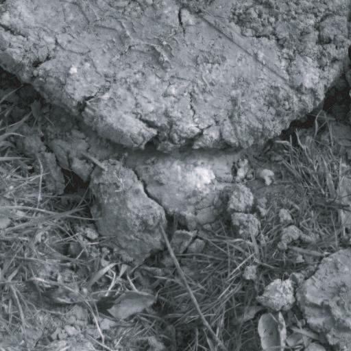
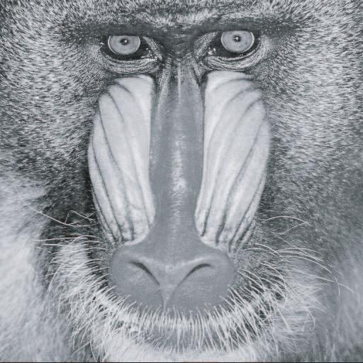
94 Figure 3.3. Ensemble of images, from Van Hateren database of calibrated images [156], and from database widely used in computer science and neural modeling efforts. 81

95 the somewhat arbitrary scaling of the input signal. One can in theory adjust the optimal σ to match the input level of the experimental stimuli. However, we have found in practice that neurons also exhibit a range of different sensitivities. So we choose different values of σ in the simulations to match the sensitivity of the cell being modeled. The value of σ controls the contrast at which the response of the neuron reaches semi-saturation, and the contrast at which the divisive gain signal is not effective in modulating the response of the model neuron; for weak signals, σ dominates the divisive equation. Changing σ is equivalent to shifting the contrast scale. Finally, we simulate each experiment, holding all weights of the model fixed. We present the model neuron with input, typically gratings that vary in some parameter. The response of the neuron is simulated by computing the normalized responses of the primary filter to the experimental stimuli. The response of the divisive neighborhood is assumed to be phase invariant, as if it is coming from either an ensemble of simple cells at a variety of phases, or from complex cells. Computationally, similar results are obtained by averaging the response over multiple phases (this would be similar to the summed response to a drifting grating), or by taking the sum of squared responses of two filters that are 9 degrees out of phase (e.g., quadrature pairs). Here we have chosen the latter solution, because it speeds up simulation time and does not alter the results Mapping out the Receptive Field As a prior step to running experiments on the model, we need to map out a receptive field. We could just measure the excitatory extent of the primary filter in our model. 82

96 However, a physiologist does not have this luxury; so we also estimate the receptive field extent, as if we do not know the structure of the model. We assume a circular receptive field, as is often done in physiology (note that this is not exactly correct for our receptive fields, but it is also not exactly correct for real cells). Ideally, we d like to choose a method for estimating the receptive field that is most comparable with the physiological data. Unfortunately, there are no uniform standards for measuring the receptive field. In general, for experiments that probe only the classical receptive field and not the surround, the exact choice of receptive field extent has not been a major issue at all, so long as the selected region drives the cell. Experimenters aiming to separate out influences of center and surround have struggled with the problem of choosing the extents appropriately. Early experiments have typically hand-fitted the receptive field based on responses to oriented bars or lights. These procedures tend to underestimate the size of the receptive field by about a factor of two relative to more recent methods (see for example [33] for a discussion). Here we follow recent physiological procedures of expanding the diameter of an optimal sine grating until a maximal response (typically 95 percent of the maximum) is achieved [43, 33, 128]. This technique is matched to all the surround experiments of Cavanaugh et al. presented in the chapter. The procedure is illustrated in figure 3.4a for our model neuron. When a grating of optimal orientation and spatial frequency is expanded in diameter, the mean response of the model neuron increases, until it reaches a peak. Subsequently, the response of the neuron declines and eventually tapers off to a minimal value. This increase and subsequent decrease of response is very typical of cells in area V1 (see for example, [33, 128]). Based on this procedure, the receptive field is mapped out 83

97 a 7 Classical RF Mean response Suppression extent Grating diameter b Mean response Numerator Denominator Grating diameter Figure 3.4. Mapping out the classical receptive field. a, Response of model neuron (from divisive normalization) to an expanding optimal sine wave grating. Arrows indicate 95 percent of the peak (corresponding to the estimated extent of the receptive field) and 95 percent of the minimal value (corresponding to the estimated suppressive effect). Procedure based on Cavanaugh et al. [33]. b, Components of the model leading to overall response in (a). Specifically, plotted are the numerator component (squared response of excitatory filter) and denominator component (sum of squared responses of the neighboring filters, with constant σ omitted in the plot). Arrows indicate same positions as in (a). 84

98 as a circular region with a diameter equal to 95 percent of the maximal value. In the model neuron, the estimated receptive field diameter spans 9 pixels (first arrow in the figure). The 95 percent minimum point following the decline in response is suggestive of the suppressive extent of the neuron [33]. In the model neuron, this point corresponds to 24 pixels (second arrow in the figure). In physiology, it is difficult to disentangle the components that lead to this behavior. But since we know the components of the model, we can examine separately the excitatory numerator component response (coming from the true primary filter) and the divisive component (coming from the weighted squared neighboring neuron responses). We ignore for now the constant σ in the divisive component and assume it is relatively small and has minimal influence on the denominator. This is a reasonable assumption, since most physiological studies have fit the receptive field with high contrast stimuli. However, we will come back to this issue later on in the chapter. Figure 3.4b illustrates the two components of the model. The numerator component is just the squared response of the primary filter. It continues to increase and reaches 95 percent of the peak at around a 14 pixel diameter. Note that this is approximately 1.5 times the estimated diameter. That is, we have underestimated the true spatial extent of the primary filter. The minor decrease in response following the peak is due to the structure of the linear filter, which has a small inhibitory sidelobe. The denominator component coming from the sum of squared responses of neighboring filters continues to increase farther out in space than the numerator component. The denominator reaches 95 percent of the maximum value at approximately 24 pixels. This is approximately 2.5 times the extent of the esti- 85

99 mated receptive field, and 1.7 times the extent of the true excitatory component. Note that the peak of the denominator component in the model (figure 3.4b) is also roughly equal to the minimum value of the overall model neural response (figure 3.4a). Thus, the overall model neural response gives a good indication of the suppressive extent in the model. Now that we ve mapped out a linear receptive field, we can proceed to compare model and physiology. We will point back to some of the issues raised here throughout the comparison Comparison to Physiology Inside the Classical Receptive Field We first demonstrate behavior of the model for stimuli presented inside the classical receptive field. Figure 3.5 shows data and model simulations of cross-orientation suppression. An optimal grating is placed inside the classical receptive field. An orthogonal mask grating is superimposed on the optimal grating (forming a plaid). Each curve in the figure indicates the response as a function of the contrast of the optimal grating, for a particular mask contrast. The sigmoidal shape of the curves results from the squaring nonlinearity and the normalization. The steepness of the model curves is determined by the fixed exponent of two, and appears to roughly match the cell. The presence of the mask suppresses the responses to the optimal grating. Specifically, the contrast response curves are shifted to the right (on a log axis), indicative of a divisive gain change. The model exhibits similar behavior, which is a direct consequence of the statistically-chosen normalization weights. Neighboring 86

100 model filters responding to the orthogonal grating exert a divisive effect on the primary filter. This, in turn, arises from the statistical properties of natural images discussed in chapter 2. Masking effects can also be observed at a single contrast, as a function of mask orientation. Figure 3.6 depicts the orientation tuning curve for a fixed optimal grating in the presence of a mask of varying orientation. As before, the optimal grating and the mask are additively combined to form a plaid. Also plotted is the orientation tuning curve for the model neuron without a mask (control). Both curves are normalized to a maximum value of 1. The mask exerts a mixture of excitatory and suppressive effects. In particular, the presence of the mask at orientations close to the optimal serves both to excite the primary filter, and to provide suppression through division. This results in a broadening of the orientation tuning curve, because the response is increased more near the optimal orientation, while the divisive component does not change as much as a function of orientation. Orientation tuning in area V1 has been a widely studied topic. One of the striking features of orientation tuning is that it appears to be invariant to the contrast of the stimulus (e.g., [13, 145], and see also [5]). Figure 3.7 depicts the orientation tuning as a function of contrast for a typical V1 cell [145] versus the model. Both the cell and model orientation tuning are roughly contrast invariant. In the context of a divisive normalization model, invariance of orientation tuning has been postulated to arise through equal weighting of the squared filter responses in the denominator [64]. If the divisive signal is equally weighted at each orientation, then the tuning of the primary filter cannot be altered. To examine the model behavior more closely, we separate out the components of numerator and 87

101 denominator (figure 3.8). The top panel depicts the same overall model response as in figure 3.7. The middle panel illustrates the two model components. The divisive denominator component is not truly flat as a function of orientation. This means that the model orientation tuning curves are only close to contrast invariance; at high contrast, the tuning is slightly sharper than at low contrast. This is possibly an artifact of the model. Specifically, the optimization procedure does not allow to include the excitatory filter or filters that are highly correlated with the excitatory filter. As a result, there is no source of self-suppression in the model (see discussion in chapter 2). Added self-suppression would help to achieve true contrast invariance. In our model, increasing the stimulus diameter would result in an added suppression at the optimal orientation. When we actually do this (bottom panel of the figure) the divisive signal is roughly constant as a function of orientation. Experimentally, it would be interesting to understand if the contrast invariance of V1 neurons holds up across stimuli of different sizes. Though contrast invariance of orientation tuning is widely published, we believe it has only been examined for certain stimulus sizes, most probably small ones that match hand-computed receptive fields [13, 145]. Perhaps cells are most optimized for orientation invariance at particular stimulus sizes. For example, if the orientation tuning of the surround suppression is more sharply tuned than the center, then very large stimuli will have added suppression at the preferred orientation, and this could potentially result in a broader tuning curve at high contrasts. But less relative suppression at the preferred orientation for small stimuli could potentially result in a sharper tuning curve at high contrasts (as in our model). Sclar and Freeman note in their paper that For only two cells, tuning patterns were marginally different from zero and 88

102 Cell (Bonds, 1989) Model Mean response Signal contrast Signal contrast Mask contrast: Figure 3.5. Cross-orientation suppression in area V1 [24]. Responses to optimal stimulus are suppressed by an orthogonal masking stimulus within the receptive field. This results in a rightward shift of the contrast response curve (on a log axis). Curves on cell data plot are fitted with a Naka-Rushton function, r(c) = c 2 /(ac 2 + b 2 ). in these cases, tuning sharpness appears, counterintuitively, to decrease slightly as contrast increases [13]. The relation between stimulus size and orientation invariance needs to be examined experimentally Mapping the Region Outside the Classical Receptive Field As stated earlier, stimuli outside the classical receptive field are useful in experimental settings, because they elicit no response in the neuron when presented alone. Nevertheless, they can modulate the response of a neuron to stimuli placed inside the classical receptive field. The region outside the classical receptive field is usually chosen as an annular ring surrounding the receptive field. Selecting the dimensionality of the annulus 89

103 Cell (Bonds, 1989) Model 1 opt + mask grating single grating opt + mask grating single grating Mean response -1 1 Grating orientation -1 1 Grating orientation Figure 3.6. Orientation masking in area V1 inside the classical receptive field [24]. Dashed line indicates response to a single grating, as a function of orientation. Solid line indicates response to an optimal grating additively superimposed on a mask grating of variable orientation. All curves are normalized to have a maximum value of one. Cell (Skottun et, 1989) al. Model Mean respone 5 Contrast: Orientation 1 Orientation Figure 3.7. Contrast invariance of orientation tuning in area V1 [145]. Cell and model are plotted such that their bandwidth is visually equated, even though the specific bandwidth differs. 9

104 a Mean Response b Mean Response Orientation Contrast: Numerator Denominator c Mean Response Orientation 8 Numerator Denominator 1 Orientation Figure 3.8. Examination of model components of orientation tuning as a function of contrast in area V1. a, Overall model response, as in figure 3.7. b, Components of the model leading to overall response in (a). Specifically, plotted are the numerator component (squared response of excitatory filter) and denominator component (sum of squared responses of the neighboring filters, with constant σ omitted in the plot). Note that denominator component is not truly constant as a function of orientation. c, Components of the model for stimulus that is twice the size of the estimated receptive field. Now the denominator component is roughly constant as a function of orientation, leading to true orientation invariance. 91

105 (and especially its most inner border) is again a rather tedious issue for physiologists. If one underestimates the surround, then it could actually exert an excitatory effect on the neuron. This effect could be particularly extreme if the surround inner annulus diameter is chosen equal to the diameter of the estimated receptive field. Remember in the model that the estimated receptive field extent was smaller than the true extent of the receptive field (figure 3.4). Moreover, estimated receptive fields using small bars or spots of light are even smaller. If special care is not taken to separate out the center and surround, the physiological results could be contaminated by interactions between these two components. Only recently, physiologists have taken more scrutiny to separate out center and surround. Cavanaugh et al. have developed a method, which we follow here, for determining the surround [33]. The method is illustrated in figure 3.9a for the model neuron. A zero-luminance hole is placed in the center. Surrounding the hole is an annular ring at the optimal orientation and frequency for the model neuron. The diameter of the hole is expanded, which is equivalent to expanding the diameter of the inner border of the annulus. Now the 95 percent minimal value is taken to represent the diameter of the inner border of the annular surround. This amounts to a 12 pixel diameter in the model neuron. An annular ring of zero luminance is then placed between the estimated center and surround. Figure 3.9b illustrates the two components of the model. Note that both the excitatory numerator and suppressive denominator decrease for larger proximal borders of the annulus, but the numerator decreases more rapidly to a minimal value. The 12 pixel diameter that was chosen based on the overall model neuron response is quite well matched to the minimal value of the numerator alone. We 92

106 a Mean response Surround b Mean response Numerator Denominator Figure 3.9. Mapping out the surround annulus inner diameter. a, Response of model neuron (from divisive normalization) to an optimal grating with a hole of zero luminance. As the hole is expanded, the proximal border of the annulus is increased. Arrow indicates 95 percent of the minimal value. Procedure based on Cavanaugh et al. [33]. b, Components of the model leading to overall response in (a). Specifically, plotted are the numerator component (squared response of excitatory filter) and denominator component (sum of squared responses of the neighboring filters, with constant σ omitted in the plot). Arrow indicates same position as in (a). 93

107 should point out that this value is almost equal to, but slightly below, the peak of the numerator of an expanding sine grating computed in figure 3.4b. The inconsistency between the two methods is a consequence of the squaring nonlinearity of the numerator kernel response. Thus, we have come close to but marginally underestimated the real inner border of the surround. That is, an optimal stimulus placed in the surround will elicit no response, as required. But the opposite is not true; a stimulus expanding from the center will still slightly increase its response as it encroaches onto the surround. Remember that the physiologist does not have access to the true extent of the presumed center component Comparison to Physiology Outside the Classical Receptive Field We now compare model responses to steady-state nonlinear physiological behaviors outside the classical receptive field. Figure 3.1 shows data from a Macaque monkey [33]. An optimal sinusoidal grating stimulus is placed inside the classical receptive field of a neuron in area V1. A mask grating is placed in the annular region surrounding the classical receptive field. Each curve in the figure indicates the response as a function of the center contrast for a particular surround contrast. Presentation of the mask grating alone does not elicit a response from the neuron, but its presence suppresses the responses to the center grating. Specifically, the contrast response curves are shifted to the right (on a log axis), indicative of a divisive gain change. When the mask orientation is parallel to the center, this shift is much larger than when the mask orientation is orthogonal to the center (Figure 3.1). 94

108 a Mean respone Cell (Cavanaugh et al., 2) Signal contrast Model Signal contrast Mask Signal Mask contrast: No mask.13.5 b Mean response Signal contrast Signal contrast Mask Signal Mask contrast: No mask.13.5 Figure 3.1. Contrast response curves for parallel versus orthogonal surround masks in area V1. cell data from [33]. a, Mean response rate of a V1 neuron as a function of contrast of an optimally oriented grating presented in the classical receptive field, in the presence of a surrounding parallel masking stimulus. Curves on cell data plots are fits of a Naka-Rushton equation with two free parameters [33]. b, Mean response rate vs. center contrast, in the presence of an orthogonal surround mask. 95

109 The model exhibits similar behavior (Figure 3.1), even though we have not fitted the model to the data. The model behavior is due to a suppressive weighting of neighboring model neurons with the same orientation preference that is stronger than that of neurons with perpendicular orientation preference (see also [144]). Note that this behavior would not be observed in previous equally weighted normalization models, because the parallel and orthogonal surround stimuli would produce the same normalization signal. The weighting in our model is determined by the statistics of our image ensemble, and is due to the fact that adjacent regions in natural images are more likely to have similar orientations than orthogonal orientations. For example, oriented structures in images (such as edges of objects) tend to extend along smooth contours, yielding strong responses in linear filters that are separated from each other spatially, but lying along the same contour (see also [6, 138]). In other experiments in V1, it has been demonstrated that for a parallel surround, more suppression is observed for aligned patches in the surround than for non-aligned patches [33]. Our model is expected to be consistent with this result, since we obtain stronger weighting for iso-oriented filters that are aligned with the primary filter, than for non-aligned filters (also see bowties in chapter 2). We have thus far examined surround suppression as a function of only two surround orientations, parallel and orthogonal to the optimal. Figure 3.11 explores a wider range of surround orientations at a single (high) contrast. The center orientation is held fixed at the optimal orientation of the neuron. Both in cell and in model, most suppression is observed when the surround stimulus is also placed at the preferred orientation of the neuron. The amount of maximal suppression is 96

110 Cell (Cavanaugh et al., 2) Model Mean response Center orientation Center orientation Surround orientationsurround orientation Figure Surround suppression as a function of orientation for optimal center stimulus in area V1. Maximum suppression is obtained when the surround orientation is also at the preferred orientation of the neuron. Model neuron is plotted with twice the number of orientation points, but marked points correspond to cell. Model is scaled to have same maximal value as cell. also very similar in model and cell. This behavior has led experimenters to wonder whether the absolute surround orientation drives the amount of suppression, or whether the relative orientation between center and surround is pertinent. It has been suggested that the amount of surround suppression depends contextually on the orientation of the grating placed in the center, consistent with the latter hypothesis. Specifically, some experimental data show that neurons appear to shift their point of maximal surround suppression to match the orientation of a grating placed in the center [139, 33]. This seems to be counterintuitive to the type of divisive normalization model we ve described, in which the point of maximal suppression ought to be fixed and determined by the weighting of the divisive pool. For example, in our model neuron, we would always expect maximal suppression for a surround stimulus with the preferred orientation 97

111 Cell (Cavanaugh et al., 2) Model a Mean response Center orientation Surround orientation Center orientation Surround orientation b Mean response Center orientation Surround orientation Center orientation Surround orientation Figure Dependence of surround suppression on center orientation in area V1. a, Surround orientation suppression when center orientation is fixed at +45 degrees from the preferred orientation of the neuron. Maximum suppression is obtained when the surround orientation is equal to the orientation of the center grating (for the cell) and shifted towards the orientation of the center grating (for the model). b, Surround orientation suppression when center orientation is fixed at -45 degrees from the preferred orientation of the neuron. Maximum suppression is obtained when the surround orientation is equal to the orientation of the center grating (for the cell) and shifted towards the orientation of the center grating (for the model). Physiological data from [33]. Model neuron is plotted with twice the number of orientation points, but marked points correspond to cell. Model is scaled to have same maximal value as cell. 98

112 a 3 Center Orientation More overlap Mean response 2 1 b Mean response Surround orientation Measured center/surround c Mean response Surround orientation Less overlap Surround orientation Figure Model dependence of surround suppression for different separations of center and surround with optimal center stimulus. a, Center stimulus 9 pixels; surround stimulus 1.5 pixels (i.e., smaller than estimated surround). b, Center stimulus 9 pixels; surround stimulus 12 pixels. (i.e., equal to estimated surround). c, Center stimulus 9 pixels; surround stimulus 16 pixels. (i.e., larger than estimated surround). In all cases, maximal suppression is achieved when the surround grating is at the preferred orientation of the model neuron. 99

113 a Mean response Center orientation More overlap b Mean response Surround orientation Measured center/surround c Surround orientation Less overlap Mean response Surround orientation Figure Model dependence of surround suppression for different separations of center and surround with non-optimal center stimulus. Center orientation is fixed at the +45 degrees away from the preferred orientation of the neuron. a, Center stimulus 9 pixels; surround stimulus 1.5 pixels (i.e., smaller than estimated surround). b, Center stimulus 9 pixels; surround stimulus 12 pixels. (i.e., equal to estimated surround). c, Center stimulus 9 pixels; surround stimulus 16 pixels. (i.e., larger than estimated surround). 1

114 of the neuron, regardless of the center stimulus orientation. We decided to test this idea through simulation in the model. Figure 3.12a illustrates cell and model mean response rate as a function of surround orientation, for a center stimulus that is fixed at +45 degrees the optimal orientation. The point of maximal suppression now shifts towards +45 degrees in the cell. In the model, the shift is not quite as extreme; a maximal suppression is seen at degrees. Note that we have sampled orientation at a finer scale in the model than in the experimental data to illustrate this point. Similar behavior is observed for a center stimulus that is fixed at -45 degrees the optimal orientation (figure 3.12b): the cell and model minimum is shift towards -45 degrees. There is also a broadening of tuning (relative to figure 3.11) in the model and (especially at -45 degrees) in the cell. The model does not behave in detail like the cell. But the fact that the model also obtains a shift toward the orientation of the center stimulus is interesting. This kind of behavior could arise if the center and surround of the model are not truly separated. In fact, center and surround are not truly separated in the model. Recall that the surround was slightly underestimated in the inner annulus expansion experiment. So stimuli placed in the surround may have a minor effect on the excitatory filter of the model. In addition, stimuli placed in the center will naturally also effect the divisive normalization signal. This is expected because the suppressive pool includes filters in the center and filters at 3 pixel displacements from the center, which would still be influenced by the spatial region of the classical receptive field. To test the hypothesis that the behavior in the model arises from incomplete 11

115 separation of center and surround, we decided to alter the separation between center and surround stimuli. That is, the center receptive field is held at the fixed estimated diameter, and the surround inner annulus diameter is modified. We either reduce (to 1.5 pixels), keep constant (12 pixels), or increase (to 16 pixels) the inner annulus diameter. Figure 3.13 depicts the behavior of the model to a center stimulus at the optimal orientation. As before, maximal suppression is obtained when the annular surround stimulus is also at the optimal orientation. This behavior is consistent for all three conditions. Figure 3.14 depicts the behavior of the model to a center stimulus shifted by +45 degrees. This time the model behaves differently in all three conditions. For smaller separation, the maximal suppression is at around +45 degrees. In contrast, for larger separation, the maximal suppression is centered approximately at the optimal orientation of the model neuron. Note that for larger separation we guarantee that the surround stimulus does not encroach on the excitatory filter. However, the center stimulus still does encroach on the suppressive filters. Analogous behavior is observed for a center shifted to -45 degrees (not shown here). We have demonstrated that incomplete separation of center and surround could lead to changes in model behavior. This is a preliminary result; whether it has bearing to neural data requires further investigation. Perhaps biology is set up such that two stimuli that closely border one another contextually shift the orientation of maximal suppression. In any case, a divisive normalization model can produce this type of effect, at least qualitatively. Cavanaugh et al. have suggested another explanation for this behavior in the context of a divisive gain model: that changing the balance between a center and surround gain (such that the center gain 12

116 # % ' )( Cell (Cavanaugh et al., 2) Model '# &% " #$ Annulus inner diameter (deg)! Figure Response as a function of surround inner diameter in area V1. Physiological data from [33]. is favored) could amount to a shift in the orientation of maximal suppression [33]. We now examine the suppressive effect of the surround as a function of spatial proximity to the center. In figure 3.15 a surround mask is placed at the optimal orientation. As the surround mask is moved farther away from the receptive field, the suppressive effect is reduced both in the cell and model neuron. As mentioned above, a motivating characteristic of normalization models has been the preservation of tuning curve shape under changes in input level. However, the shapes of physiologically measured tuning curves for some parameters exhibit dependence on input level [128, 76, 33]. Figure 3.16 shows an example of this behavior in a neuron from primary visual cortex of a Macaque monkey [33]. The graph shows the response of the cell as a function of the radius of a circular patch of sinusoidal grating, at two different contrast levels. The high-contrast responses 13

117 are generally larger than the low-contrast responses, but in addition, the shape of the curve changes. Specifically, for higher contrast, the peak response occurs at a smaller radius. The same qualitative behavior is seen in the model neuron, although weaker than in the physiological cell. The behavior in the model is a result of two competing factors: primary filter excitation and neighboring filter suppression. At high contrasts, the suppressive signal modulates the shape of the tuning curve of the primary filter. Recall figure 3.4, in which neighboring filters that are spatially displaced relative to the primary filter reduce the excitatory response of the primary filter through division. This results in both a shift of the peak to a smaller diameter, and a continued decline in response following the peak. But at low contrasts, the tuning function is primarily determined by the excitatory numerator component, because σ dominates the divisive gain signal. So the tuning as a function of radius is more matched to the linear tuning properties of the primary filter Cell and Model Variations in area V1 We have modeled the behaviors of typical cells, but there are quantitative differences amongst individual cells. Figure 3.17 shows an example of variation across cells in physiological recordings in V1. In this figure, the amount of suppression for a parallel and orthogonal surround varies across the population. Amount of suppression is computed as the response of the neuron to an optimal grating inside the classical receptive field together with a surround mask (either parallel or orthogonal to the optimal orientation), divided by the response of the neuron to an optimal grating and no surround mask. This value is computed for high contrasts 14

118 Cell (Cavanaugh et al., 2) Model Mean response Diameter (deg.) Contrast: Diameter (deg.) Figure Nonlinear changes in tuning curves as a function of stimulus diameter for different input levels in area V1. Plotted is the mean response rate of a V1 neuron as a function of stimulus radius for two different contrasts [33]. The peak response radius for both cell and model is smaller for the higher contrast. 15

119 of the stimulus and mask. Each point in the graph corresponds to data from a single cell. A large proportion of the cells show substantially more suppression when the preferred orientation is in the surround than when the orthogonal orientation is in the surround. Note that some of the cells also exhibit facilitation due to the surround, although suppression is much more prominent. Variations can also arise in the model. One source of variation in the model is observed when the divisive weights are optimized for different images. Figure 3.18 demonstrates the amount of suppression for a parallel versus orthogonal surround. Each point in the figure corresponds to a simulation with weights computed from a single image. Overall we ran simulations over 4 different images. The model follows a similar trend to the physiological data; there is more suppression when the preferred orientation is in the surround than when the orthogonal orientation is in the surround. The gray arrow in the figure points to the values obtained with the weights from the image ensemble used throughout the chapter. Figure 3.19 shows that images from the Van Hateren versus the standard image data set follow a similar distribution. White noise, in contrast, yields roughly the same amount of suppression for parallel and orthogonal surround. The definition of natural images is quite loose. Some images in the set yield points away from the prominent data cloud, although these too still exhibit more suppression for the parallel than for the orthogonal surround. Shown in the figure are two such images, that appear rather texture-looking. Textures (both artificial and natural) are likely to have more variant statistics than so-called natural scenes (see also [11]). We have illustrated one possible source of model variation, but variations in 16

120 the model may also arise from other factors, such as the choice of primary and neighborhood filters. We have chosen one primary filter in the model, and compared simulation results to neurons with different tuning properties. We have thus assumed invariance with respect to frequency and orientation. Images are roughly spatial frequency invariant, and we have verified that modifying the spatial frequency of the primary filter does not alter the qualitative results in the chapter. However, we believe that images are not orientation invariant; for example, vertical, horizontal and diagonal orientations probably do not appear with equal probability in nature. We are beginning to investigate how the results vary with orientation of the primary filter. Preliminary examination suggests that the qualitative nature of the simulations in the chapter does not change. However, the strength of the suppression, and relative contributions of aligned and non-aligned positions are likely to change. Since we also do not have a detailed account of changes in physiology as a function of neuron orientation and frequency, the assumption of invariance in the model is not unreasonable. These two sources of variation, experimental and model, are very different; it is difficult to directly compare between them. There are numerous possible explanations for the variations that arise in physiological recordings, including cells from different animals; different layers; with different tuning properties; and (perhaps) one can also hypothesize that different cells are optimized for different subclasses of images. 17

121 2 Normalized response, parallel surround Normalized response, orthogonal surround Figure Distribution of physiological recordings from different cells, for parallel versus orthogonal surround in area V1. Each point corresponds to data from a single cell. The x axis is the response of the neuron to a center optimal grating with an orthogonal surround, divided by the response of the neuron to the center grating alone. The y axis is the response of the neuron to a center optimal grating with a parallel surround, divided by the response of the neuron to the center grating alone. Most points in the graph lie below the unit slope line, indicating that there is more suppression for parallel surround than for orthogonal surround. 18

122 Normalized response, parallel surround Normalized response, orthogonal surround Figure Distribution of model simulations with weights computed for different natural images, for parallel versus orthogonal surround. Each point corresponds to a simulation with weights computed for a single image. The x axis is the response of the model neuron to a center optimal grating with an orthogonal surround, divided by the response of the model neuron to the center grating alone. The y axis is the response of the model neuron to a center optimal grating with a parallel surround, divided by the response of the model neuron to the center grating alone. Most points in the graph lie below the unit slope line, indicating that there is more suppression for parallel surround than for orthogonal surround. The gray arrow points to simulation results for the image ensemble used in the chapter. 19

123 Normalized response, parallel surround noise Standard Images Normalized response, orthogonal surround Figure Distribution of model simulations with weights computed for different natural images, for parallel versus orthogonal surround (part 2). Same as Figure 3.18, but we plot separately simulation results from the Van Hateren image database and the standard image database. Also shown is a simulation with Gaussian white noise. Unlike the images, the white noise simulation yields roughly the same suppression for parallel and orthogonal mask gratings (lying close to the unit slope line). 11