CRUSTAL STRUCTURE OF SOUTHEASTERN TANZANIA

Transcription

1 The Pennsylvania State University The Graduate School College of Earth and Mineral Sciences CRUSTAL STRUCTURE OF SOUTHEASTERN TANZANIA A Thesis in Geosciences by Alysa J. Young 2012 Alysa J. Young Submitted in Partial Fulfillment of the Requirements for the Degree of Master of Science December 2012

2 The thesis of Alysa J. Young was received and approved* by the following: Andrew A. Nyblade Professor of Geosciences Thesis Advisor Charles J. Ammon Professor of Geosciences Peter C. LaFemina Assistant Professor of Geosciences Chris Marone Professor of Geosciences Associate Department Head of Graduate Program in Geosciences * Signatures are on file in the Graduate School. ii

3 Abstract The structure of Jurassic to Neogene coastal basins along the Tanzania passive margin and crustal thickness beneath them have been investigated in this thesis using P-wave receiver functions and Rayleigh wave phase and group velocities. Seismic data recorded by eight stations deployed from February 2010 through July 2011 provide the primary dataset. Receiver functions have been computed using ~100 teleseismic events with epicentral distances of The resulting waveforms, consisting of several Ps arrivals in the first 5s, indicate complicated basin structure. To estimate crustal thickness, an application of the H- stacking method was attempted for each station. Well-resolved results from one station located on basement rock yield crustal thickness of approximately 38km, with an average Vp/Vs of Sediment-filled basins below the other stations produce a seismogram ringing effect that masks the Moho Ps arrival and have been interpreted using other methods, including a joint inversion of the receiver functions, phase, and group velocities and forward modeling of the receiver function waveforms. Phase and group velocities were taken from other studies and were incorporated only in the joint inversion method. Results, where well determined, indicate basin thicknesses of 3km to 5.5km and Moho depths of ~38km. Within the basins, the top ~2km are found to have high Poisson s ratio (~0.40) with average shear wave velocity of ~1.5km/s, which are characteristics consistent with the Jurassic and younger marls and clays that outcrop in the basins. The velocity models also indicate that the next 1-3km have an average shear wave velocity of ~2.5km/s, most likely representing Karoo units comprised of fluvial siltstones and sandstones. The average crustal thickness beneath the basins is consistent with crustal structure away from the basins, indicating little, if any, crustal thinning. Little crustal thinning is also supported by a beta factor (stretching factor) of 1.1, which was calculated for the crust beneath the basins. iii

4 Table of Contents List of Figures...vi List of Tables...x Acknowledgements...xi 1.0 Introduction Background Geological Setting and Tectonic History Geology at Station Locations Previous Studies Data and Methodology Data Receiver Functions Dispersion Curves Methods H-κ Stacking Forward Modeling of Travel Times Forward Modeling of PRF Waveforms Joint Inversion Uncertainty Results The Receiver Functions Modeling Results Station WALE Station IFAK Station CHAL Station MANG Station MOHO Station KIMA Station INDI 31 iv

5 4.2.8 Station MTWA Discussion The Coastal Basins The Crust Stations with a Gradational Moho Conclusions...49 References...50 Appendix A: List of teleseismic events used in computation of receiver functions...54 Appendix B: Plots of radial (left) and transverse (right) receiver functions as a function of ray parameter versus time 57 Appendix C: H- stacking results for Station WALE at different P-wave velocity values...64 Appendix D: Supplemental joint inversion results..65 v

6 List of Figures Figure 1. Crustal cross-section from Novak et al. [1997] along the refraction line in SE Kenya from near Nairobi (shotpoint ATH) to the Indian Ocean (shotpoint IND) (see Figure 2 for location). Numbers on the cross-section are P-wave velocities in km/s.2 Figure 2. Topographic map of East Africa that shows the main tectonic framework, permanent and temporary seismic stations, and the KRISP (Kenya Rift International Seismic Project) refraction line [Novak et al. (1997)]. The box outlines the study area (Figure 3).4 Figure 3. Geologic map of SE Tanzania showing the structures relevant to this study (modified after the Geological Survey Division, Dodoma [1959]). The labeled red triangles show the eight broadband station locations of the AfricaArray Basin Experiment ( 10-11). The color-coded dots represent the nodes at which dispersion curves were extracted for Station WALE, two backazimuths (BAZ) of Station IFAK, and the coastal stations. The continental shelf location is approximated from topographic data of the region....6 Figure 4. Geologic map of the Ifakara region, modified from the compilation map by the Geological Survey Division, Dodoma [1962]. The location of station IFAK is shown by an inverted red triangle...8 Figure 5. Geologic map of the area around Station CHAL (red inverted triangle), modified from the compilation map by the Geological Survey Division, Dodoma [1960]...9 Figure 6. Geologic map of the Kilwa Masoko region (modified after the compilation map by the Geological Survey Division, Dodoma [1963]). Station KIMA (red inverted triangle) is on Pleistocene to recent sediments, east of the Cretaceous to Paleogene units...10 vi

7 Figure 7. Map showing locations of earthquakes used in this study, centered on the middle of the seismic network. Numbers on the circles give the epicentral distance (in degrees) from the center of the seismic network..13 Figure 8. Plot showing three average dispersion curves along coastal Tanzania: the average of the coastal nodes in Figure 3 south of -8.5, the average of the those nodes north of -8.5, and the average of all of the nodes. The error bars on the green line show +/-1 standard deviation of the mean. 15 Figure 9. Cartoon illustrating the P-wave receiver function that would be generated in response to a simple layer over half-space model. The direct P arrival is narrow and has the largest amplitude. It is followed by the P-to-S conversion with the associated multiples..17 Figure 10. Examples of the receiver functions for a) Station WALE using a Gaussian of 1.0 (PPRFs are shown in red) and b) Station CHAL using a Gaussian of 2.5 and , 23 Figure 11. H- κ stacking results for Station WALE. The numbers along the top summarize the results and the contours on the plot map out the percentage values calculated from the objective function. To the left of each receiver function, the top number gives the backazimuth and the bottom number gives the event distance in degrees. The bottom number allows differentiation between PRFs and PPRFs because PPRFs were calculated using events for > Figure 12. Joint inversion results for Station WALE. The text in the top left summarizes the influence and smoothing parameters, as well as the value of κ and layer thickness (in parentheses) for the two top layers of the velocity model. The top left plot shows the receiver functions, stacked by ray parameter. The range of ray parameters is to the left of each waveform and the backazimuth for individual receiver functions vii

8 within a stack are listed below the stack. The plot in the bottom left shows the dispersion curves and the two plots on the right display the velocity profile...32 Figure 13. Joint inversion result for Station IFAK using a) data from events sampling the Kilombero rift and b) data that samples the basement rock north of the seismic station. See Figure 12 for description of features in the plot..33, 34 Figure 14. Joint inversion result for Station CHAL. See Figure 12 for description of features in the plot..35 Figure 15. Joint inversion result for Station MANG. See Figure 12 for description of features in the plot. The error bars on the top right velocity profile show the uncertainty of +/-0.2km/s to outline the large range of possible Moho depths at this station Figure 16. Joint inversion result for Station MOHO. See Figures 12 and 15 for description of features in the plot Figure 17. Joint inversion result for Station KIMA. See Figures 12 and 15 for description of features in the plot.38 Figure 18. Joint inversion result for Station INDI. See Figure 12 for description of features in the plot..39 Figure 19. Joint inversion result for Station MTWA. See Figures 12 and 15 for description of features in the plot Figure 20. Simplified version of the geology map in Figure 3 with a summary of results at each station. The top number is total basin thickness and the bottom number is the Moho depth at each station. Grey italicized numbers indicate results that were not well-determined. Colors on the map are based on shear-wave velocities that have viii

9 been determined for different rock types [e.g. Castagna et al., 1985; Christensen, 1996; Newhouse et al., 2004]...41 Figure 21. a) Example from Station CHAL of utilizing the final joint inversion velocity model to forward model the receiver functions layer by layer (only layer models that caused significant waveform changes are shown). b) Example of labeling main arrivals in the 2.5 and 5.0 receiver function stacks (one ray parameter) used in the joint inversion for Station CHAL Figure 22. a) Map of the Bouguer corrected gravity anomaly in Africa from Tugume et al. [2012]. b) Map of the same area with gravity derived crustal thickness in kilometers.46,47 Figure 23. Stack of the receiver function stacks used in the joint inversion for the stations along the coast, calculated at three Gaussian width parameters. Note the shoulder on the right side of the direct P arrival in the top panel.48 ix

10 List of Tables Table 1. Summary of the forward modeling parameters..18 Table 2. Summary of changes in basin and crustal structure changing the assumed Poisson s ratio and influence factor. Final parameters that were used are in bold 21 Table 3. The results of this study are summarized in this table. Note that Moho depth is the crust and basin thickness..25, 26 x

11 Acknowledgements I would like to thank all of the AfricaArray participants who helped collect the data used in my research, in particular Gabriel Mulibo, Jordi Julia, and Mtelela Khalfan who collected the data from the southeastern Tanzania basins. I also want to thank my adviser, Andrew Nyblade, for all of his support and guidance, my committee members Charles Ammon and Peter LaFemina, and all of my research group and fellow graduate students. xi

12 1.0 Introduction In this thesis, I document my investigation of the basin and crustal structure in southeastern Tanzania using broadband seismic data from eight AfricaArray seismic stations. The purpose of this thesis is to 1) investigate the structure of the Mesozoic to Cenozoic sedimentary basins along the coast and 2) estimate how much crustal thinning has occurred beneath them. Eastern Africa has experienced multiple episodes of rifting since the late Paleozoic, the first of which resulted in the development of Karoo (Permian-Triassic) basins as thick as 6-10km. The coastal basins investigated in this study are Jurassic to recent in age, potentially containing Karoo sediments in the subsurface, and are not well-studied. The crust beneath the study area was formed in the Neoproterozoic and the structure is, again, not well known. A refraction profile from southeastern Kenya suggests up to 20km of crustal thinning towards the coast (Figure 1) [Novak et al., 1997]. However, looking at the data indicates that crustal thickness is not certain near the coast. Also, there is no other evidence for large amounts of crustal thinning in the region. In order to address the primary goals of this research, P-wave receiver functions and Rayleigh wave group and phase velocities are used to model the structure beneath the AfricaArray basin network. At each of the seismic stations, P-wave receiver functions are calculated from teleseismic events (30-90 ) that were recorded between February 2010 and July The receiver functions at each station were interpreted by one or more modeling techniques, including: the H- stacking method [Zhu and Kanamori, 2000], joint inversion of the receiver functions and Rayleigh wave dispersion velocities [Julia et al., 2000], and forward modeling of the receiver function waveforms [e.g. Langston, 1997]. The thickness, shear wave velocity, and Poisson s ratio ( ) were determined for stations in the basins, revealing ~2km of sediments with high Poisson s ratio overlying ~2km of older sediments. In addition, the thickness and average shear wave velocity of the crust were determined for all of the stations. The results of this study place new constraints on the evolution of the crust in southeastern Tanzania, indicating that the basins are quite shallow and that little, if any, crustal thinning has occurred. The basins are found to be between 3km and 5.5km thick, 1

13 while crustal thickness in the area is ~38km. The crustal thickness found here is consistent with estimates of crustal thickness away from the basins, but not with the Novak et al. [1997] study that suggested as much as 20km of thinning seaward. Figure 1. Crustal cross-section from Novak et al. [1997] along the refraction line in SE Kenya from near Nairobi (shotpoint ATH) to the Indian Ocean (shotpoint IND) (see Figure 2 for location). Numbers on the cross-section are P-wave velocities in km/s. 2

14 2.0 Background 2.1 Geological Setting and Tectonic History The Archean Tanzania Craton forms the core of the Precambrian framework in East Africa and is surrounded by a number of Proterozoic mobile belts (Figure 2). To the southeast and southwest of the craton are the Paleoproterozoic Usagaran and Ubendian Belts, respectively, to the west and northwest are the Mesoproterozoic Kibaran and Rwenzori Belts, respectively, and to the east is the Neoproterozoic Mozambique Belt. The study area lies within the Mozambique Belt, which formed through multiple collisional events between 1200 and 450 Ma, resulting in mainly north-to-south striking structures and intense folding and metamorphism [e.g. Key et al., 1989; Schluter, 1997]. Superimposed on the Precambrian tectonic framework are three episodes of Phanerozoic rifting. Karoo rifting (Permian to Triassic) affected large regions of eastern and southern Africa and was caused by intraplate transtensional deformation associated with stresses from the northern and southern margins of Gondwana [Delvaux, 2000]. Karoo sedimentation continued until the Early Jurassic in southeastern Tanzania rift basins, which have been suggested as influential to the location of Gondwana s crustal failure along east Africa [Delvaux, 2001]. Rifting between Africa and Madagascar commenced in the Mid- Jurassic from the North (contemporaneous with the initial breakup of Eastern and Western Gondwana) and was finished by the Late Cretaceous [Coffin and Rabinowitz, 1987]. Subsidence and eastward regional tilting associated with the transtensional deformation and extension occurred up until the Late Cretaceous when the passive margin along eastern Africa had fully developed. A third episode of rifting occurred in the Cenozoic, resulting in the present day East Africa Rift system. Many Cenozoic rift basins formed in the eastern and western branches of the rift system (Figure 2), some of them within or adjacent to Karoo rifts [e.g. Nyblade, 2002]. Much work has been done on the Karoo sequences to the west and south of the study area, in which up to 6-10 km of Karoo sediments (primarily of deltaic-lacustrine and fluvial origin) have been mapped [e.g. Kreuser, 1984; Hankel, 1987; Verniers et al., 1989; Kreuser, 1995; Schluter, 1997]. Terrestrial sediments of the Late Carboniferous-Permian in eastern 3

15 Figure 2. Topographic map of East Africa that shows the main tectonic framework, permanent and temporary seismic stations, and the KRISP (Kenya Rift International Seismic Project) refraction line [Novak et al. (1997)]. The box outlines the study area (Figure 3). 4

16 Tanzania were deposited in northeast trending depressions, parallel to the existing basement fabric. The Lower Karoo includes glacial deposits from the Permo/Carboniferous Gondwana glaciation, as well as fluvial and/or lacustrine sandstones and silts with carbonaceous horizons and coal-bearing beds. They are overlain by arkoses and continental red beds, which are in turn overlain by carbonaceous shales and thick lacustrine series. During the Triassic, very thick fluvial-deltaic sandstones and siliciclastics were deposited, making up the main graben filling units. Kreuser [1984] wrote of five Karoo NNE-trending grabens in eastern Tanzania and noted that some Karoo sediment was unconformably overlain by Jurassic sediments and that there was no thick post-jurassic deposition. However, Roberts et al. [2010] note some significant sandstone beds from the Cretaceous-Paleogene associated with the fluvial systems draining the inland highlands. Along the coast, there was much erosion of and overlapping of marine beds onto the Karoo units during the mid-jurassic transgression. This was followed by a progradation of fluvio-deltaic series eastward during the development of the passive margin through to the Cretaceous, which culminated in restricted marine conditions, characterized by the deposition of silty shales and grey-green marine clays and marls (~2km reported) [Schluter, 1997; Kreuser, 1995]. Tectonic stability lasted into the Early Tertiary, with grey clays, silty layers and local marl bands being deposited along the passive margin [Schluter, 1997]. There was then intense tilting and rapid subsidence along the coast in the Late Paleogene, resulting in Neogene inland elevation and, in turn, increased sediment volume to the coast [Schluter, 1997]. This tectonic reactivation continued with broad tilting and folding in the Neogene and faulting throughout the Miocene and mid Pleistocene. Cenozoic faulting on the coast included the formation of the east-west trending Ruvu and Rufiji Troughs, both of which bound Pre-Tertiary basins [Nicholas et al., 2007] (Figure 3). Faulting in the Mozambique Belt interior during the Cenozoic was oriented primarily north-west-south-east. Reactivation of Karoo faults is observed as well, such as in the connection of the Kilombero extensional zone with Lake Malawi s rift basins [Le Gall et al., 2004]. The Kilombero Rift (Figure 3) is northeast-southwest trending and the main border faults are believed to be reactivated Karoo faults [e.g. Kent et al., 1971; Dypvik et al., 2001; Le Gall et al., 2004]. 5

17 6

18 2.2 Geology at Station Locations The eight broadband stations of this study are located in southeastern Tanzania (Figure 3). The stations will be discussed clockwise, starting inland with Station WALE, then Station IFAK, and then north to south along the coast. More is known about the geology around some stations than others. Station WALE is near the town of Liwale, just east of exposed Karoo sedimentary rocks. The station is located on rocks of the Mozambique Belt. Station IFAK (Ifakara) is in the Kilombero River valley, but Precambrian outcrops in the north and south valley walls indicate that crystalline rock (basement) lies beneath the exposed Quaternary alluvium, cemented sands, and gravels [Geological Survey Division, Dodoma, 1962] (Figure 4). Station CHAL is outside the town of Chalinze in the Ruvu basin, sitting on Cretaceous grey-green marls of unknown thickness. Just to the west are Jurassic calcareous sandstones and siltstones. Basement outcrops about 10km west of the station (Figure 5). Schluter [1997] noted that there is a discontinuity of Jurassic strata on Precambrian strata (no Karoo) north of Chalinze. Station MANG is within the town of Maneromango in a Cretaceous basin southeast of the Ruvu basin and ~70 km from the coast (Figure 3). The basin is surrounded by alluvium and Neogene-Paleogene sediments. The geology around the station is not well-documented. Station MOHO (Mohoro) is located in the Rufiji Trough, in an area where Quaternary alluvium outcrops (Figure 3). The geology around the station is also not well documented, but because it is along the coast where Jurassic-Cretaceous sediments outcrop, units of those ages may be present in the subsurface. The Kilwa Masoko-Lindi region (Stations KIMA and INDI, respectively) is characterized by sands, clays, and marls (Figure 3). Drilling in the 1960s found greater than 1700m of Lower Tertiary grey clays and sands. There are also Pliocene or Quaternary reef limestones in the area up to 25m thick (Kilwa Bay) [Schluter, 1997]. Station KIMA is in the Mandawa Basin, sitting on Pleistocene-to-recent sands and silts with Cretaceous and/or Jurassic outcrops to the west (Figures 3, 6). Nicholas et al. [2007], using seismic sections and previous drilling results, reported a basin stratigraphy dominated by clays with thin limestone and sandstone beds. They also reported claystones overlain by unconsolidated clays in the near-surface geology. 7

19 8

20 9

21 10

22 Station INDI is on the eastern edge of Cretaceous sediments in the northeastern Ruvuma Basin (Figure 3). Nicholas et al. [2007] found that here Miocene clays are overlain by thick limestones. At both locations (KIMA and INDI), there may be Karoo deposits in the subsurface. About 40m of Jurassic red and grey sandy marls alternating with soft yellowish sandstone is observed between the towns [Schluter, 1997]. Station MTWA (Mtwara) is in the southeastern part of the Ruvuma Basin that lies within Tanzania (Figure 3). Schluter [1997] noted that there is about 1100m of Miocene clays and limestones in the basin near Mtwara. Nicholas et al. [2007] found Plio-Pleistocene units of sand and gravels at Mtwara that were not observed in the northern Ruvuma Basin or Mandawa Basin. 2.3 Previous Studies The crustal structure of the Mozambique Belt has been well characterized by a number of studies using receiver functions and surface wave dispersion measurements. Last et al. [1997] studied the crustal structure of seven stations in the Mozambique Belt using receiver functions and Rayleigh wave phase velocities in a grid search modeling method. They found Moho depths of 36-39km, an average crustal shear wave velocity (Vs) of 3.74km/s, and Poisson s ratios ranging from 0.24 to Julia et al. [2005], in a similar study using a joint inversion of receiver functions and surface wave dispersion, found crustal thicknesses in the Mozambique Belt of 36 to 40km, an upper crust with Vs of km/s, and upper mantle shear wave velocities of km/s. Dugda et al. [2005] used P-wave receiver functions and surface wave dispersion calculated from the Kenya broadband experiment [Nyblade and Langston, 2002] to determine crustal structure in Kenya. They determined a Moho depth of 37 to 42km and a crustal Poisson s ratio between 0.24 and 0.27 for the Mozambique Belt. Tugume et al. [2012] obtained an average Moho depth of 37+/- 3km, an average crustal Vs of 3.6km/s, and an average mantle Vs of 4.4km/s for the Usagaran Belt. The Usagaran Belt lies just to the west of the Mozambique Belt in southwestern Tanzania and so it is important to note the similarity to the Mozambique Belt results discussed here. The only seismic refraction results of crustal structure for the Mozambique Belt near the coast come from Novak, et al. [1997] in southern Kenya. The refraction line was part of 11

23 the Kenya Rift International Seismic Project (KRISP) and was 420km long, oriented northwest-southeast with ~100km shot spacing (Figures 1,2). They infer a possible seaward crustal thinning from a thickness of ~42km inland to ~23km at the coast, but the thickest crust that is well imaged in the refraction profile is ~33km thick, ~80km inland from the coast. In the aforementioned study by Last et al. [1997], results for the station closest to the coast (HALE, northeastern-most station in Tanzania in Figure 2; about 40km inland) indicate a Moho depth of 39+/-4km. 3.0 Data and Methodology Data Earthquakes were recorded from February 2010 through July 2011 on eight broadband seismometers, comprising the AfricaArray SE Tanzania basin experiment (Figures 2 and 3). The main components of each station included a broadband sensor (Guralp CMG40T, Guralp CMG3T, or Streckeisen STS-2), a 24-bit RefTek datalogger, and a GPS clock. Data were recorded continuously at 40 samples per second. Teleseismic events with epicentral distances of and magnitudes of 5.0 or greater recorded on these stations have been used in this study (Figure 7 and Appendix A). This study is part of a larger project in eastern Africa: the AfricaArray East African Broadband Seismic Experiment (AAEASE). Receiver functions are only computed for the 8 stations in southeastern Tanzania, but dispersion curves attained from all of the AAEASE stations are used in this study. The data for the AAEASE were recorded between August 2007 and July 2011 on broadband seismometers in Uganda, Tanzania, and Zambia (Figure 2). For periods of 8-30s, group velocities were determined using ambient seismic noise tomography [Boyle, 2012] and for periods of s, phase velocities from a two plane wave approximation method were used [Adams et al., 2012]. More details on the dispersion curves are discussed below. 12

24 Figure 7. Map showing locations of earthquakes used in this study, centered on the middle of the seismic network. Numbers on the circles give the epicentral distance (in degrees) from the center of the seismic network Receiver Functions Receiver functions (RFs) are a powerful tool in determining the seismic velocity structure beneath a station. Cassidy et al. [1992] determined that they can resolve boundaries with shear wave velocity contrasts as low as 0.2km/s, layers as thin as 2-3km, and they typically sample crustal structure 5-15km from the receiver. Where sediments are present, the amplitude of the resulting reverberations may be up to 10 or 20 times the amplitudes of the deeper crustal phases [Langston, 2011], decreasing the amount of interpretable phases and to an extent, the resolution. P-wave receiver functions were computed in this study using the iterative, time domain deconvolution technique in which the vertical component of the seismogram is deconvolved from the radial and transverse components to produce a signal of P-to-S converted phases whose timing and amplitudes are dependent on local structure [Ligorría and Ammon, 1999]. The seismograms were first decimated to 10 samples per second and cut to 5 seconds before and 100 seconds after the first P arrival. The data were then filtered between 13

25 8 and 0.05 Hz to cut out high and low frequency noise, respectively, and the horizontal components were rotated into the great circle path to obtain radial and transverse components. The data were filtered at different frequency ranges, but Hz represented the data well. The resulting waveforms were used in the iterative deconvolution. A maximum number of 500 iterations were used to obtain optimal results [Ligorría and Ammon, 1999]. Receiver functions were computed using 1000 iterations, but the waveforms were not significantly different and they produced consistent results as those of 500 iterations. For each event, a radial and transverse receiver function was computed, each at five different low-pass Gaussian filter parameters: 0.5, 1.0, 2.5, 5.0, and These Gaussian filter width parameters control the respective frequency content of the waveform: 0.15, 0.30, 0.75, 1.5, and 3.0 Hz. The lower frequencies are good for observing prominent phases from the lower crust and mantle, while the higher frequency RFs can reveal details of shallow crustal structure. The receiver functions were next analyzed for quality. First, an automated least squares misfit was calculated between the original radial seismogram and that of the vertical component convolved with the radial receiver function (a back-calculated radial seismogram). A similarity of 75% or greater between the radial and back-calculated radial was used to high grade the receiver functions for further analysis. In addition, events for which the transverse receiver functions exhibited large amplitudes were disregarded. Large amplitudes on the transverse receiver function suggest anisotropy and/or heterogeneity, complicating extractable information from the radial receiver function [e.g. Cassidy, 1992]. The best quality RFs were binned according to ray parameter and stacked. For any station with overall poor data quality and/or availability, PP receiver functions (PPRFs) were computed as well. They were computed the same way as the P-wave RFs (PRFs), except that earthquakes in the distance range were used, with waveforms cut around the PP phase instead of the first P arrival Dispersion Curves The group velocities at periods 8s to 30s were determined from Rayleigh waves extracted from ambient seismic noise recorded by all of the seismic stations shown in Figure 2 [Boyle, 2012]. Boyle [2012] tomographically produced group velocity maps at periods of 14

26 8, 10, 15, 20, 25, and 30s. Group velocities at nodes shown in Figure 3 were used to compute an average dispersion curve representative of the region around the station(s). The nodes for station WALE are east of the station in order to avoid group velocities representative of the neighboring Karoo basin to the west. Station IFAK had receiver functions at two sets of backazimuths and, therefore, has two different groups of nodes. Finally, for the six stations along the coast, nodes averaged along all of the coastal basins were used. Figure 8 illustrates that there is consistency in the group velocity for the nodes across the coastal basins. The phase velocities reported by Adams et al. [2012] were used at each of the eight stations for periods of 25s to 100s. Phase velocities from within half a degree of each station were averaged and used in conjunction with the group velocities and receiver functions for interpretation. Figure 8. Plot showing three average dispersion curves along coastal Tanzania: the average of the coastal nodes in Figure 3 south of -8.5, the average of the those nodes north of -8.5, and the average of all of the nodes. The error bars on the green line show +/-1 standard deviation of the mean. 15

27 3.2.0 Methods Three methods of modeling RFs have been used and are described here: H-κ stacking, forward modeling, and joint inversion H-κ Stacking This method was developed by Zhu and Kanamori [2000] to find optimal values of crustal thickness (H) and Vp/Vs ratio (κ) using receiver functions that have a clear Ps phase from the Moho and from one or more multiples (e.g. PpPms and PpSms+PsPms) (Figure 9). In this method, the receiver functions are transformed from the time domain to H-κ parameter space via the use of an objective function, s(h,κ), and a summation procedure which consists of summing the weighted phases amplitudes at predicted arrival times (and assumed P-wave velocity (Vp)) for varying values of H and κ: (1) Where w 1, w 2, w 3 are the weights for each phase amplitude (r j ) of arrival time t (1,2,3), and N is the number of receiver functions. Arrival times are calculated with the equations discussed in the following section (3.2.2). When s(h,κ) reaches its maximum, optimal values of H and κ have been determined for a simple crustal model [Zhu and Kanamori, 2000]. Variables in the H-κ stacking include the specific weights and Vp. The sum of the three weights must equal 1.0, with the clearest phase receiving the highest weight. Formal uncertainties of H and κ can be obtained using a bootstrapping method of repeating the summation many times with a random resampled dataset [Efron and Tibshirani, 1991]. 16

28 Figure 9. Cartoon illustrating the P-wave receiver function that would be generated in response to a simple layer over half-space model. The direct P arrival is narrow and has the largest amplitude. It is followed by the P-to-S conversion with the associated multiples Forward Modeling of Travel Times Zandt et al. [1995] and Last et al. [1997] discuss calculating crustal thickness based on arrival times of the direct P-arrival, the Moho Ps, and its two multiples, PpPms and PpSms+PsPms. There are four equations that are utilized in this study to forward model travel times of converted phases: t Ps t P = H [(Vs -2 p 2 ) 1/2 (Vp -2 p 2 ) 1/2 )] (2) t PpP t Ps = 2H(Vp -2 p 2 ) 1/2 (3) t PpS+PsP t P = 2H(Vs -2 p 2 ) 1/2 (4) κ = {(1 p 2 Vp 2 ) [2(t Ps t P )/(t PpP t Ps ) + 1] 2 + p 2 Vp 2 } 1/2 (5) where t Ps is the arrival time of a Ps conversion from a discontinuity, t PpP and t PpS+PsP are arrival times from the multiples, H is the thickness of the layer, and p is the ray parameter. Equation 2 is useful for estimating H if a reliable velocity model is available. Equations 3 and 4 can be used for approximating multiple arrival times when the arrivals are 17

29 masked by reverberations, and Equation 5 can be used to estimate κ when the other variables are known with some certainty Forward Modeling of PRF Waveforms Forward modeling of receiver function waveforms was performed using three programs that have been developed by Owens [1984], Randall [1989], and Ammon [1991]: icmod for creating a velocity model, respknt for calculating the seismic response to the input velocity model based on Kennett s [1983] reflection matrix method, and pwaveqn for computing the synthetic receiver function by using Langston s [1979] source equalization approach. Parameters that were used with these codes are summarized in Table 1. Table 1. Summary of the forward modeling parameters. Variable Parameters Set Parameters layer thickness 0.1 sampling Interval p wave velocity 60s signal duration s wave velocity ~0.05s/km slowness (κ and σ) full multiples density mode conversions included Gaussian bandwidth 0 trough filler 5s phase shift Computing a best-fit synthetic waveform by varying the variable parameters and visually comparing each synthetic RF to the data was attempted for each station. This was done to approximate local structure. Also, forward modeling can be used for identifying peaks in the RFs by building a resulting joint inversion velocity model layer by layer Joint Inversion Julia et al. [2000] developed a method of jointly inverting receiver functions and dispersion curves for estimating the Vs structure beneath a station. The input consists of an initial model, receiver functions, and a dispersion curve of group and/or phase velocities. An influence factor (between the two datasets) and smoothing parameters are also needed in the 18

30 inversion to ensure a smooth model that optimally fits the data. The receiver functions were stacked according to ray parameter for up to two different frequencies. The generation of the receiver functions was described in section 3.1.1, and dispersion curves were taken from Boyle [2012] and Adams et al. [2012], as explained in Section The linearized inversion uses a damped least-squares algorithm and results in a 1-D Vs depth profile that best fits the data. Each dataset has a relative weight controlled by the influence factor in the joint minimization of the L2 norm of the vector residuals of each dataset [Julia et al., 2000]. Using receiver functions at different frequencies helps to distinguish between sharp and gradual features [Julia, 2007], and dispersion curves over a large range of periods help in constraining average Vs into the mantle. The PREM model [Dziewonski and Anderson, 1981] with a modified crust was used as the starting model, with slight changes (primarily in the first two kilometers) made for each station. The first 1-2 kilometers were composed of km thick layers to allow for imaging thinner basin layers, then km thick layers to ~6km depth, 2.5km thick layers to ~52km depth, 5.0km thick layers until 247km depth and 25km thick layers at deeper depths. The inversion was performed to a depth of ~187km and fixed to the PREM model below that to account for the partial sensitivity of long-period dispersion velocities to deeper structure [Julia et al., 2003]. Layer thickness increases with depth because of the decreased resolution available in the dispersion curves at higher periods. Moho depth was at approximately 38km (plus-or-minus the varying basin thickness) in the starting model. The depth at which Vs exceeded 4.3km/s was used to define the Moho because this value is representative of mantle material [Christensen and Mooney, 1995; Christensen, 1996]. Poisson s ratio in the crust was set to 0.26 (κ = 1.75), increasing through the mantle, and remains fixed throughout the inversion process. Where sediments are present, the velocity model was allowed to have at least two layers of high Poisson s ratio and low velocity to fit the RF waveforms. The κ values between 1.73 ( = 0.25) and 3.33 ( = 0.45) and layer thickness between 0.2km and 3km were tested for the top two layers of the velocity model for each of the stations in a sedimentary basin. Generally, sediments will be defined as having a Vs 2.9km/s, which can be affirmed by previous studies such as Zelt and Ellis [1999], where all of the stations except two on basement have near-surface velocities below 2.9km/s. Also, Vs values of 0.12 to 19

31 2.8km/s are reported for young sediments, clays, shales, and sandstones [e.g. Castagna et al., 1985; Newhouse et al., 2004] while values of 3.0 to 4.2km/s are reported for crystalline rocks [e.g. Christensen, 1996]. The influence factor controlling the weight of each dataset and the smoothing factor that can be applied throughout depth were experimented with and values of 0.5 and 0.3 were used, respectively, unless mentioned otherwise in section 4. An influence factor of 0.5 optimally represented the two datasets and a smoothing factor of 0.3 provided enough smoothing to the model to constrain the inversion without loosing too much fit to the data. Extra smoothing can be applied per layer in the velocity model. The value is relative and is multiplied by the smoothing factor in the joint inversion process (which is also a relative value). The values used are 1 for the first ~8km and 5 below that, unless otherwise mentioned in section 4. Density (rho) is specified for each layer and it was calculated from the compressional velocity (Vp) based on Berteussen s [1977] empirical relation for lower crustal rocks: rho = (0.32 * Vp) (6) Equation 6 was used throughout the starting model, but Gardner et al. [1974] derived a relation between Vp and rho specifically for sedimentary rocks, which holds for 1.5 < Vp < 6.1 km/s: rho = 1.74Vp 0.25 (7) This relationship is more appropriate for basin geology and was used for any layers with Vp < 6 km/s Uncertainty Assuming plane layered structures are appropriate, the uncertainty in joint inversion results have been investigated by other studies using receiver functions with clear Moho phases [e.g. Julia et al., 2005; Kgaswane et al., 2009; Tugume et al., 2012]. By recomputing the inversion multiple times with varying weighting parameters, constraints, and Poisson s ratio, the uncertainty in crustal Vs was found to be no greater than 0.2km/s. This uncertainty 20

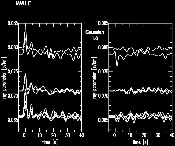
32 in crustal Vs leads to an uncertainty in Moho depth of no more than 3km. Limited testing of how the inversion parameters affect crustal Vs results in this study indicate a similar sensitivity to the selection of parameters and, therefore, in Moho depth estimates. Table 2 summarizes the changes in basin and crustal structure, introduced by varying both the Poisson s ratio and the influence factor. Varying Poisson s ratio from 0.25 to 0.31 is appropriate based on the compilation of laboratory measurements of lower and middle crustal rocks by Rudnick and Fountain [1995]. Table 2. Summary of changes in basin and crustal structure changing the assumed Poisson's ratio and influence factor. Final parameters that were used are in bold. Poisson's Ratio Avg Basin Vs Avg Crustal Vs Basin Thickness Moho Depth (km/s) (km/s) (km) (km) Influence Factor Results 4.1 The Receiver Functions The receiver functions used for each station are shown in Appendix B. A Gaussian width factor of 1.0 produced the RFs with the clearest Moho Ps for the two stations on basement (WALE, IFAK), while for stations in the coastal basins, RFs at 2.5 and 5.0 have been used because the higher frequency content assists in the interpretation of basin structure. Example RFs are shown in Figure 10a,b for Station WALE (on basement) and Station CHAL (on sediments). Stations on high Poisson s ratio sediments have characteristic waveforms of a broad, small amplitude direct P arrival, followed by a large amplitude sediment-bedrock Ps arrival and reverberations. Large amplitudes on the transverse RFs suggest shallow 3D structure complexity, as explained in section

33 a) Radial Transverse 22

34 b) Radial Transverse Figure 10. Examples of the receiver functions for a) Station WALE using a Gaussian of 1.0 (PPRFs are shown in red) and b) Station CHAL using a Gaussian of 2.5 and

35 4.2 Modeling Results The modeling results for each station are reviewed in this section and summarized in Table 3. Joint inversion results for each station are shown together in figures listed at the end of this section (Figures 12-19), followed by a map that spatially summarizes the results (Figure 20). Crustal thickness beneath the coastal basins, where it can be determined, is similar to other areas of the Mozambique Belt. For the joint inversion procedure, basin thickness is determined by the layers in the final inversion model with Vs 2.9km/s, while crustal thickness is determined by those layers with Vs < 4.3km/s (see section 3.2.4). The same model parameterization was used for each station below the variable top two layers. As described in section 3.2.4, the thickness and of the top two layers were systematically varied in a trial-and-error fashion to find a best fitting model. The inversion was sensitive to 0.5km changes in the layer thickness and changes in of 0.05 in the two top layers and were, therefore, the step-sizes used in varying thickness and, respectively Station WALE A sufficient number of good quality RFs with a large direct P-arrival and a clear Moho Ps for Station WALE were obtained from P and PP phases to enable the use of the H- method. Based on the visual quality of RFs, weights of 0.8, 0.2, and 0.0 were used for Ps, PpPms and PpSms+PsPms, respectively. Vp was set to 6.5 km/s as a representative value for Precambrian crust [e.g. Christensen and Mooney, 1995; Julia et al., 2005]. Varying the velocity between 6.3 and 6.7 km/s yielded variations in optimal Moho depth of ~3km and in optimal of ~0.01. A crustal thickness of 37.7+/-3km and a of 1.67+/-0.07 (corresponding to a = 0.22+/-0.04) were obtained (Figure 11). Results using a Vp of 6.3 and 6.7 km/s are provided in Appendix C. A joint inversion of RFs and dispersion measurements was also performed for Station WALE (Figure 12) and the result was consistent with the H- stacking results. The top layers of the best fitting model were 1km each with of ~1.75. No smoothing was applied. Crustal thickness was determined with this method to be at ~35km depth with an average crustal Vs of 3.6km/s. 24

36 Table 3. Summary of study results. Note that Moho Depth is the crust and basin thickness. 3a. The Crust Station Lat Long Elevation Moho Depth Avg Crust Vs κ σ Method (deg) (deg) (m) (km) (km/s) (crust) (crust) WALE / / / / ,2 IFAK / ,3 CHAL / MANG MOHO KIMA INDI / MTWA Method 1 = H- stack 2 = joint inversion 3 = Ps travel time 25

37 3b. The Basin Station Basin H Total Basin H Avg Basin Vs κ σ (km) (km) (km/s) (high σ seds) (high σ seds) high σ seds/older seds high σ seds/older seds WALE N/A N/A N/A N/A N/A IFAK 0 / / 2.2 N/A N/A CHAL 2 / / MANG 2.5 / / MOHO 0 / / 2.7 N/A N/A KIMA 2.5 / / INDI 2 / / MTWA 3.5 / /

38 Figure 11. H- κ stacking results for Station WALE. The numbers along the top summarize the results and the contours on the plot map out the percentage values calculated from the objective function. To the left of each receiver function, the top number gives the backazimuth and the bottom number gives the event distance in degrees. The bottom number allows differentiation between PRFs and PPRFs because PPRFs were calculated using events for >

39 4.2.2 Station IFAK The H- stacking method could not be applied at Station IFAK due to a lack of clear Moho multiples in the receiver functions. Despite calculating PP receiver functions to supplement the dataset, the two resulting ray-parameter-binned RFs had waveforms that were too different from each other to perform a single joint inversion. The lower ray parameter waveforms (backazimuths toward the Kilombero Rift) had one more arrival in the first five seconds than those of the higher ray parameter (backazimuths to the north) and the joint inversion could not produce a solution that would fit both waveform types. Instead, a joint inversion was performed for each backazimuth set, using the individual receiver functions instead of stacks, along with the respective group velocity curves (specific group velocity curves discussed in Section 3.1.2) (Figure 13a,b). The RFs with N-NE backazimuths, jointly inverted with the group velocities representative of the Kilombero rift valley, and the phase velocities result in a Moho depth of 38+/-3km and an average crustal Vs of 3.7km/s. The RFs at these backazimuths also sampled sediments, which the joint inversion results indicate are ~1km thick with average Vs of 2.2km/s. There is a high velocity zone between about 2km and 6km depths that the inversion needs to match the large peaks and troughs in the first 5s of the RFs. These high velocities are also present in the joint inversion result of the second set of RFs, and are probably not real. The second set of RFs had backazimuths to the north. The joint inversion resulted in a Moho depth of 40km+/-3km and an average crustal Vs of 3.7km/s. There was no indication of sediments in this velocity profile. Forward modeling using travel times was also carried out. Using nearby values of Vp and from Tugume et al. [2012], Equation 2 was used to calculate Moho depth based on t Ps. Assuming a Vp of 6.5km/s and an average of 1.75 ( = 0.26), a crustal thickness (H) of 35-41km was determined. The range of thicknesses comes from calculating H at different values of (1.75+/-0.05) and t Ps (4.6+/-0.3s). 28

40 4.2.3 Station CHAL Figure 14 shows the data and joint inversion results for Station CHAL. Like most of the basin stations, the RFs in the first 5s are complicated, though the ringing in the waveform is not as intense as typical basin receiver functions. Synthetic testing indicated that this is most likely due to a lower velocity contrast at the sediment-bedrock interface. The first 3s of the RFs include a direct P arrival at 0s and a larger amplitude peak at ~1s, followed by one or two peaks between 2s and 5s. The model providing the best fit to the data contained two top layers, each 2km thick, and both with a of 2.30 ( of ~0.38). The total resulting basin thickness was 4km with an average Vs of 1.6km/s for the high Poisson s ratio sediments and 2.6km/s for the deeper sediments. A Moho depth of 37+/-3.0km and an average crustal Vs of 3.8km/s were obtained. A test on starting model sensitivity was performed by varying the initial Moho depth by +/-5km and showed variability within the crustal thickness uncertainty of +/-3km. Moving the initial Moho depth up 5km resulted in essentially the same velocity profile, while moving it down 5km resulted in the same velocity profile up to ~25km depth. Below 25km, the velocities were slightly different than those of the final model for the original Moho depth, and the Moho depth was 1-2km deeper. The results are shown in Appendix D Station MANG Within the first four seconds of the RFs from Station MANG, the direct P is immediately followed by a peak of larger amplitude, a very large downswing, and then a peak with the largest amplitude of the RF. There is no clear Moho Ps among the RF stacks. The model providing the best fit to the data consisted of a top layer that was 1.5km thick with a of 2.50 and a second layer that was 1km thick with a of Smoothing of 0.3 was applied throughout the model, with extra smoothing (values ranging from 5 to 8; refer to section for details on extra smoothing) applied between the depths of ~38km and ~55km to constrain the inversion. The average Vs in the high Poisson s ratio sediments is 1.5km/s and is 2.6km/s for the underlying sediments. The Moho in the final model is not well-resolved and can lie anywhere between 30km and 50km depths where the velocity is between 4.2km/s and 4.3km/s (Figure 15). Average Vs in the crust above 30km is 3.6km/s. 29

41 4.2.5 Station MOHO The RFs from Station MOHO are simpler in the first few seconds than the RFs from other coastal stations. The direct P has the largest amplitude of the waveform, and especially in the RFs of Gaussian 2.5, is followed by fairly unstable reverberations. Again, there is no clear phase associated with the Moho Ps. Figure 16 shows the joint inversion results for Station MOHO. The model resulting in the best fit to the data had the two top layers at 1km each with a of Smoothing was applied at a value of 0.3 throughout depth. The narrow, larger amplitude direct P arrival indicates that there are no high Poisson s ratio sediments beneath the station and this was affirmed by the joint inversion result. The final model had 3km of the higher velocity sediments (Vs ~2.7km/s) overlaying the crust (average Vs ~3.6km/s). The results, like for Station MANG, indicate a gradational Moho, with the Moho lying between 25km and 41km (4.2km/s Vs < 4.3km/s) Station KIMA The first five seconds of the RFs from Station KIMA have peaks that are almost symmetrical about the arrival of largest amplitude at ~2s. The direct P is very small and is not fit well by the joint inversion. As with most of the other stations RFs, there are many reverberations and no clear Moho Ps. The receiver functions were not being fit well by the inversion process and the influence factor was consequently increased to 0.8 (i.e., more weight was given to the dispersion curves). The model that optimally fit both datasets included the two top layers of high Poisson s ratio sediments: a 1.5km thick layer with a of 2.80, overlying a 1.0km thick layer with a of A smoothing parameter of 0.3 was used with extra smoothing (values ranging from 5 to 7) below the basin, especially concentrated on depths ~38-46km to stabilize the inversion. The joint inversion results for station KIMA indicate a basin that contains 2.5km of high Poisson s ratio sediments (Vs ~1.3km/s) and 3km of underlying sediments (Vs ~2.3km/s). The results also yield a gradational Moho in the depth range of 28-38km, and an average crustal Vs of 3.9km/s. 30

42 4.2.7 Station INDI Station INDI s RFs have large amplitude reverberations and a large trough just before 3s, followed by the Moho Ps. Otherwise, they have the same broad direct P arrival with a larger amplitude sediment-bedrock Ps arrival at about 1s. The model that best fit the data consisted of two, 1km layers of high Poisson s ratio (a of 2.80 and 2.54, respectively) (Figure 18). Smoothing was set to 0.3 with extra smoothing applied between 3 and 20km (to a value of 5) as well as below 40km (values between 5 and 7). The final basin structure included the 2km of high Poisson s ratio sediments with an average Vs of 1.5km/s, overlying 2km of older sediments with an average Vs of 2.6km/s. The Moho depth is 38+/-3km and the average Vs in the crust is 3.8km/s Station MTWA The first five seconds of the RFs for Station MTWA consist of a very small amplitude direct P arrival and are dominated by a peak of very large amplitude at ~2.5s. No Moho Ps is observed. To model the data, the influence factor was set to 0.8 in order to place more weight on the dispersion curves during the inversion process because a good fit to the receiver functions could not be obtained (Figure 19). The starting model that resulted in the best possible fit to both datasets was a 500m thick top layer with a of 2.33 over a 3km thick layer with a of Smoothing was at a value of 0.5 for this station. Although the arrival times of phases within the first five seconds were reasonably matched, amplitudes were not. The model suggests that the basin is comprised of 3.5km of high Poisson s ratio sediments with an average Vs of ~2.4km/s, and 1km of underlying sediments that have an average Vs of ~2.6km/s. These results also suggest a Moho depth between 30- and 40km and an average crustal Vs of 3.8km/s. 31

43 Figure 12. Joint inversion results for Station WALE. The text in the top left summarizes the influence and smoothing parameters, as well as the value of κ and layer thickness (in parentheses) for the two top layers of the velocity model. The top left plot shows the receiver functions, stacked by ray parameter. The range of ray parameters is to the left of each waveform and the backazimuth for individual receiver functions within a stack are listed below the stack. The plot in the bottom left shows the dispersion curves and the two plots on the right display the velocity profile. The mantle velocities are not well-constrained, but are not important in this study. 32

44 a) 33

45 b) Figure 13. Joint inversion result for Station IFAK using a) data from events sampling the Kilombero rift and b) data that samples the basement rock north of the seismic station. See Figure 12 for description of features in the plot. 34

46 Figure 14. Joint inversion result for Station CHAL. See Figure 12 for description of features in the plot. 35

47 Figure 15. Joint inversion result for Station MANG. See Figure 12 for description of features in the plot. The error bars on the top right velocity profile show the uncertainty of +/-0.2km/s to outline the large range of possible Moho depths at this station. 36

48 Figure 16. Joint inversion result for Station MOHO. See Figures 12 and 15 for description of features in the plot. 37

49 Figure 17. Joint inversion result for Station KIMA. See Figures 12 and 15 for description of features in the plot. 38

50 Figure 18. Joint inversion result for Station INDI. See Figure 12 for description of features in the plot. 39

51 Figure 19. Joint inversion result for Station MTWA. See Figures 12 and 15 for description of features in the plot. 40

52 41

53 5.0 Discussion 5.1 The Coastal Basins A characteristic feature of the RFs from the coastal basins is a broad, low amplitude direct P arrival, followed by a larger amplitude sediment-bedrock Ps with reverberations that make it difficult to detect the Moho Ps. To illustrate that through careful modeling the Moho Ps can be identified in some cases, Figure 21a,b shows the results of forward modeling of the RFs from Station CHAL. Taking the final velocity model from the joint inversion and using the forward modeling technique discussed in Section 3.2.3, a synthetic RF can be computed layer by layer. Figure 21a includes example synthetics from this process that show when in the RF (i.e., what depth) which major phases arrive. Although the synthetic calculation will compute reverberations, they are not pronounced in Figure 21a. This is because the velocity contrast at the sediment-bedrock interface is not large enough in the model to produce large amplitude reverberations. Figure 21b illustrates how these phases can, in turn, be interpreted. For Ps phases that were determined, the arrival times of the respective multiples were calculated using Equations 3 and 4 and also labeled. The basins beneath Stations CHAL, MANG, KIMA, INDI, and MTWA have been modeled using two layers of high Poisson s ratio sediments overlaying a few layers of older sediments, and basin thicknesses have been estimated to be between 3km and 5.5km. Each station displays the same characteristic direct P arrival followed by a larger amplitude Ps arrival from the sediment bedrock interface, and many subsequent reverberations. To fit these waveforms, a of is needed for the high Poisson s ratio sediments, which is reasonable for clays, marls, or very porous sediments [e.g. Meissner, 1965; Kahler and Meissner, 1983; Sheehan et al., 1995]. This is consistent with the Jurassic-Cretaceous marls that outcrop along the coast. These sediments are 2-3km thick with average Vs ranging from 1.3km/s to 2km/s. The sediments in the lower 1-3km of the basins have an average Vs of km/s (and the of 0.26 that was assumed throughout the remainder of the velocity model). Kim et al. [2009] found subsurface Karoo units with a Vs of 2.25km/s in their study of the Rukwa Rift. Also, a maximum Vs of 2.49km/s is reported for clay-rich sedimentary rocks by Brocher [2005]. Therefore, the average Vs of older sediments (~2.5km/s) in the southeastern 42

54 Tanzania coastal basins could indicate the presence of Jurassic-Cretaceous sandstones, as well as the conglomerates, shales, and fluvial sandstones and siltstones of the Karoo. Figure 21. a) Example from Station CHAL of utilizing the final joint inversion velocity model to forward model the receiver functions layer by layer (only layer models that caused significant waveform changes are shown). b) Example of labeling main arrivals in the 2.5 and 5.0 receiver function stacks (one ray parameter) used in the joint inversion for Station CHAL. 43

55 5.2 The Crust The primary finding of this study is that crustal thickness, where it was well determined (Stations WALE, IFAK, CHAL, INDI) is consistent across southeastern Tanzania. Within the uncertainties of the Moho depth estimates, there is little, if any, crustal thinning towards the ocean in this region with an average Moho depth of ~38km and an average crustal Vs of 3.8km/s. The consistent crustal shear wave velocities indicate similar crustal composition across southeastern Tanzania as well. This result is very different from the refraction profile in Kenya [Novak et al., 1997] showing almost 20km of crustal thinning toward the Indian Ocean. However, in that profile, the Moho is only clearly imaged ~80km inland from the coast, and at that location the Moho depth is ~33km. Gravity results from Tugume et al. [2012] do not support 20km of thinning in southeastern Tanzania either (Figure 22a,b). Last et al. [1997] found the crust beneath their easternmost station (HALE) to be 39+/-4km thick, and Julia et al. [2005] obtained a similar thickness of 38+/-3km. Our results in southeastern Tanzania are in agreement with crustal thickness beneath Station HALE, and when compared to the average thickness of Mozambique Belt crust (~39km) [compilation reported by Tugume et al., 2012] indicate that there could be no more than a few kilometers of crustal thinning along the coast, if any. To support this finding, the beta factor (i.e. the stretching factor) was calculated for the crust beneath the basins with the equation from Watts [2001]: Y = T c (1-(1/β s )) * [(ρ m -ρ c )/(ρ m -ρ w )] (8). Where Y is sediment thickness (the load), T c is initial crustal thickness, β s is the beta factor, ρ m is the mantle density, ρ c is the density of the crust, and ρ w is the density of the sediments. Knowing that β s = T c /H (9), (recall that H is the present crustal thickness), we replace T c with Hβ s and rearrange Equation 8 to be 44

56 β s = [Y(ρ m -ρ w )/H(ρ m -ρ c )] + 1 (10). Using the following values, Y = 4km H = 38km ρ m = 3400kg/m3 ρ c = 2750kg/m3 ρ w = 2500kg/m3 a beta factor of ~1.1 is obtained which, with an H of 38km, implies an original crustal thickness of ~42km (by the relationship of Equation 9). Tugume et al. [2012] reported some Moho depths of 40km for the Mozambique Belt, and so a beta factor of about 1.1 is plausible for the coastal basins. In addition, the uncertainties in Moho depth estimates are ~3km, and so this would allow for several kilometers of crustal thinning that could go undetected by this study. 45

57 a) 46

58 b) Figure 22. a) Map of the Bouguer corrected gravity anomaly in Africa from Tugume et al. [2012]. b) Map of the same area with gravity derived crustal thickness in kilometers. 47

59 5.2.1 Stations with a Gradational Moho Stations MANG, MOHO, KIMA, and MTWA have joint inversion results that are not fully well-resolved, but may suggest a gradational Moho. This could result from the Moho Ps in the RFs being obscured and therefore not imaged, or else it could be real. That is, there could be no sharp compositional boundary between the crust and Moho at these locations. The stacked receiver functions used in the joint inversion process for the stations along the coast were stacked all together at Gaussian width parameters of 1.0, 2.5, and 5.0 (Figure 23) to test whether or not an average Moho Ps would become more clear. The shoulder on the direct P arrival (observed on the lowest frequency waveform) could be associated with a gradational Moho or it could be smeared reverberations. Therefore, no discernable Moho Ps is observed. Figure 23. Stack of the receiver function stacks used in the joint inversion for the stations along the coast, calculated at three Gaussian width parameters. Note the shoulder on the right side of the direct P arrival in the top panel. 48

60 6.0 Conclusions The structure of Mesozoic to Cenozoic sedimentary basins in southeastern Tanzania and that of the crust beneath them have been investigated in this thesis. P-wave receiver functions have been computed and modeled both independently and jointly with Rayleigh wave phase and group velocities. Results from Stations WALE, IFAK, CHAL, and INDI are the most reliable. The velocity models indicate that the basins have ~2km of high Poisson s ratio (~0.40) sediments with an average Vs of ~1.5km/s, overlying 1-3km of sediments that have an average Vs of ~2.5km/s. The top few layers require the high Poisson s ratio in order to fit the complex first five seconds of the receiver function waveforms. The high Poisson s ratio sediments are likely the local outcropping marls and clays, while the deeper sediments probably represent the fluvial siltstones and sandstones of the Karoo. With uncertainties included, crustal thickness beneath the basins varies from 34km to 41km and average crustal shear wave velocity is ~3.8km/s. Uncertainties in crustal thickness and Vs are +/-3km and +/- 0.2km/s, respectively. These results are similar to estimates of crustal thickness away from the basins, which suggests that there is little change in crustal thickness towards the oceanic crust. Based on the average crustal and basin structure, a beta factor of 1.1 is obtained for the crust beneath the basins, also indicating little crustal thinning. Results for stations MANG, MOHO, KIMA, and MTWA are less definitive due to the masked Moho phases in the receiver functions. Shear wave velocity is consistent with the other stations, but crustal thickness lies anywhere between 25km and 50km. These stations (besides Station MTWA) do, however, provide constraints on basin structure. 49

61 References Adams, A., A.A. Nyblade, and D. Weeraratne. Upper mantle shear wave velocity structure beneath the East African Plateau: Evidence for a deep, plateau-wide low velocity anomaly. Geophysical Journal International (2012): 189, Ammon, C. J. The Isolation of Receiver Effects from Teleseismic P-Wave-Forms. Bulletin of the Seismological Society of America 81.6 (1991): Berteussen, K. A. Moho Depth Determinations Based on Spectral-Ratio Analysis of Norsar Long-Period P-Waves. Physics of the Earth and Planetary Interiors 15.1 (1977): Boyle, K. Crustal shear-wave velocity structure of Tanzania from ambient seismic noise tomography. The Pennsylvania State University: a Masters thesis in progress (2012). Brocher, T. A. Empirical Relations between Elastic Wavespeeds and Density in the Earth's Crust. Bulletin of the Seismological Society of America 95.6 (2005): Cassidy, J. F. Numerical Experiments in Broad-Band Receiver Function-Analysis. Bulletin of the Seismological Society of America 82.3 (1992): Castagna, J. P., M. L. Batzle, and R. L. Eastwood. Relationships between Compressional- Wave and Shear-Wave Velocities in Clastic Silicate Rocks. Geophysics 50.4 (1985): Christensen, N. I. Poisson's Ratio and Crustal Seismology. Journal of Geophysical Research-Solid Earth 101.B2 (1996): Christensen, N. I., and W. D. Mooney. Seismic Velocity Structure and Composition of the Continental-Crust - a Global View. Journal of Geophysical Research-Solid Earth 100.B6 (1995): Coffin, M. F., and P. D. Rabinowitz. Reconstruction of Madagascar and Africa - Evidence from the Davie Fracture-Zone and Western Somali Basin. Journal of Geophysical Research-Solid Earth and Planets 92.B9 (1987): Delvaux, D. Tectonic and paleostress evolutuion of the Tanganyika-Rukwa-Malawi rift segment, East African Rift System.- In: P.A. Ziegler, W. Cavazza & A.H.F. Robertson (eds.), PeriTethyan Rift/Wrench Basins and Passive Margins. Memoir of the Museum National d Histoire Naturelle (Paris), Paris. (2000). Delvaux, D. Karoo rifting in western Tanzania: precursor of Gondwana break-up? Contributions to Geology and Paleontology of Gondwana, Cologne (2001): Dugda, M. T., A.A. Nyblade, J. Julia, C.A. Langston, C.J. Ammon, and S. Simiyu. Crustal Structure in Ethiopia and Kenya from Receiver Function Analysis: Implications for Rift Development in Eastern Africa. Journal of Geophysical Research-Solid Earth 110.B1 (2005). Dypvik, H., O. Hankel, O. Nilsen, C. Kaaya, E. Kilembe. The Lithostratigraphy of the Karoo Supergroup in the Kilombero Rift Valley, Tanzania. Journal of African Earth Sciences 32.3 (2001): Dziewonski, A. M., and D. L. Anderson. Preliminary Reference Earth Model. Physics of the Earth and Planetary Interiors 25.4 (1981): Efron, B., and R. Tibshirani. Statistical-Data Analysis in the Computer-Age. Science (1991): Gardner, G. H. F., L. W. Gardner, and A. R. Gregory. Formation Velocity and Density - Diagnostic Basics for Stratigraphic Traps. Geophysics 39.6 (1974):

62 Hankel, O. Lithostratigraphic Subdivision of the Karoo Rocks of the Luwegu Basin (Tanzania) and Their Biostratigraphic Classification Based on Microfloras, Macrofloras, Fossil Woods and Vertebrates. Geologische Rundschau 76.2 (1987): Julia, J. Constraining Velocity and Density Contrasts across the Crust-Mantle Boundary with Receiver Function Amplitudes. Geophysical Journal International (2007): Julia, J., C. J. Ammon, and R. B. Herrmann. Lithospheric Structure of the Arabian Shield from the Joint Inversion of Receiver Functions and Surface-Wave Group Velocities. Tectonophysics (2003): Julia, J., C.J. Ammon, R.B. Herrmann, A.M. Correig. Joint Inversion of Receiver Function and Surface Wave Dispersion Observations. Geophysical Journal International (2000): Julia, J., C. J. Ammon, and A. A. Nyblade. Evidence for Mafic Lower Crust in Tanzania, East Africa, from Joint Inversion of Receiver Functions and Rayleigh Wave Dispersion Velocities. Geophysical Journal International (2005): Kahler, S., and R. Meissner. Radiation and Receiver Pattern of Shear and Compressional Waves as a Function of Poisson s Ratio. Geophysical Prospecting 31.3 (1983): Kajato, H. K. Gas Strike Spurs Search for Oil in Tanzania. Oil & Gas Journal (1982). Kennett, B.L.N. Seismic wave propagation in stratified media. Cambridge University Press, University Printing Services, ANU (1983). Kent, P.E., M.A. Kunt, and M.A. Johnstone. The geology and geophysics of coastal Tanzania: Institute of Geological Sciences, Geophysical Papers (1971): v. 6, 101 p. Key, R. M., T.J. Charsley, B.D. Hackman, A.F. Wilkinson, C.C. Rundle. Superimposed Upper Proterozoic Collision-Controlled Orogenies in the Mozambique Orogenic Belt of Kenya. Precambrian Research (1989). Kgaswane, E. M., A.A. Nyblade, J. Julia, Phgm Dirks, R.J. Durrheim, M.E. Pasyanos. Shear Wave Velocity Structure of the Lower Crust in Southern Africa: Evidence for Compositional Heterogeneity within Archaean and Proterozoic Terrains. Journal of Geophysical Research-Solid Earth 114 (2009). Kim, S., A. A. Nyblade, and C. E. Baag. Crustal Velocity Structure of the Rukwa Rift in the Western Branch of the East African Rift System. South African Journal of Geology (2009): Kreuser, T. Karroo Basins in Tanzania. Ed. Lerkx, J.K. and Michot, J. African Geology (1984). Kreuser, T. Hydrocarbon Habitat in Rift Basins: Rift to drift evolution in Permian-Jurassic basins of East Africa. Ed. Lambiase, J.J. Geological Society (1995): Langston, C. A. Structure under Mount Rainier, Washington, Inferred from Teleseismic Body Waves. Journal of Geophysical Research 84.NB9 (1979): Langston, Charles A. Wave-Field Continuation and Decomposition for Passive Seismic Imaging under Deep Unconsolidated Sediments. Bulletin of the Seismological Society of America (2011): Last, R. J., A.A. Nyblade, C.A. Langston, T.J. Owens. Crustal Structure of the East African Plateau from Receiver Functions and Rayleigh Wave Phase Velocities. Journal of Geophysical Research-Solid Earth 102.B11 (1997): Le Gall, B., L. Gernigon, J. Rolet, C. Ebinger, R. Gloaguen, O. Nilsen, H. Dypvik, B. Deffontaines, A. Mruma. Neogene-Holocene Rift Propagation in Central Tanzania: 51

63 Morphostructural and Aeromagnetic Evidence from the Kilombero Area. Geological Society of America Bulletin (2004): Ligorria, J. P., and C. J. Ammon. Iterative Deconvolution and Receiver-Function Estimation. Bulletin of the Seismological Society of America 89.5 (1999): Meissner, R. P- and SV-waves from uphole shooting, Geophysical Prospecting 13 (1965): Newhouse, M.W., R.T. Hanson, C.M. Wentworth, R.R. Everett, C.F. Williams, J.C. Tinsley, T.E. Noce, and B.A. Carkin. Geologic, water-chemistry, and hydrologic data from multiple-well-monitoring sites and selected water-supply wells in the Santa Clara Valley, California U.S. Geol. Surv. Scient. Invest. Rep. (2004): , 142pp. Nicholas, C. J., P.N. Pearson, I.K.D. McMillan, P.W. Ditchfield, J.M. Singano. Structural Evolution of Southern Coastal Tanzania since the Jurassic. Journal of African Earth Sciences 48.4 (2007): Novak, O., C. Prodehl, A.W.B. Jacob, W. Okoth. Crustal Structure of the Southeastern Flank of the Kenya Rift Deduced from Wide-Angle P-Wave Data. Tectonophysics (1997): Nyblade, A.A. Crust and upper mantle structure in East Africa: Implications for the origin of Cenozoic rifting and volcanism and formation of magmatic rifted margins, in Menzies, M.A., Klemperer, S.L., Ebinger, C.J., and Baker, J., eds., Volcanic Rifted Margins: Boulder, Colorado, Geological society of America Special Paper 362 (2002): Nyblade, A.A., and C.A. Langston. Broadband seismic experiments probe the East African rift, EOS Trans. AGU, 83 (2002): Prodehl, C., K. Fuchs, and J. Mechie. Seismic-Refraction Studies of the Afro-Arabian Rift System - a Brief Review. Tectonophysics (1997). Randall, G. E., Efficient calculation of differential seismograms for lithospheric receiver functions, Geophys. J. Int., 99 (1989): Roberts, E. M., P.M. O Connor, N.J. Stevens, M.D. Gottfried, Z.A. Jinnah, S. Ngasala, A.M. Choh, R.A. Armstrong. Sedimentology and Depositional Environments of the Red Sandstone Group, Rukwa Rift Basin, Southwestern Tanzania: New Insight into Cretaceous and Paleogene Terrestrial Ecosystems and Tectonics in Sub-Equatorial Africa. Journal of African Earth Sciences 57.3 (2010): Rudnick, R. L., and D. M. Fountain. Nature and Composition of the Continental-Crust - a Lower Crustal Perspective. Reviews of Geophysics 33.3 (1995): Schluter, T. Geology of East Africa, Berlin; Stuttgart; Borntraeger, Germany, Druckerei zu Altenburg GmbH (1997). Sheehan, A. F., G.A. Abers, C.H. Jones, A.L. Lernerlam. Crustal Thickness Variations across the Colorado Rocky-Mountain from Teleseismic Receiver Functions. Journal of Geophysical Research-Solid Earth 100.B10 (1995): Tugume, F., A.A. Nyblade and J. Julia. Moho depths and Poisson s ratios of Precambrian crust in east Africa: evidence for similarities in Archean and Proterozoic crustal structure. Submitted to Earth and Planetary Science Letters. Revised version submitted June 28, Verniers, J., P.P Jourdan, R.V. Paulis, L. Frascaspada, F.R. Debock. The Karroo Graben of Metangula Northern Mozambique. Journal of African Earth Sciences 9.1 (1989): Watts, A.B. Isostacy and Flexure of the Lithosphere. The press syndicate of The University of Cambridge. Cambridge, United Kingdom (2001):

64 Zandt, G., S. C. Myers, and T. C. Wallace. Crust and Mantle Structure across the Basin and Range Colorado Plateau Boundary at 37-Degrees-N Latitude and Implications for Cenozoic Extensional Mechanism. Journal of Geophysical Research-Solid Earth 100.B6 (1995): Zelt, B. C., and R. M. Ellis. Receiver-Function Studies in the Trans-Hudson Orogen, Saskatchewan. Canadian Journal of Earth Sciences 36.4 (1999): Zhu, L. P., and H. Kanamori. Moho Depth Variation in Southern California from Teleseismic Receiver Functions. Journal of Geophysical Research-Solid Earth 105.B2 (2000):

65 Appendices Appendix A: List of teleseismic events used in computation of receiver functions. Year.JulianDay.Hr.Min Longitude Latitude Depth (km) Magnitude

66

67

68 Appendix B: Plots of radial (left) and transverse (right) receiver functions as a function of ray parameter versus time. 57

69 58

70 59

71 60

72 61

73 62

74 63

75 Appendix C: H- stacking results for Station WALE at different P-wave velocity values. 64