T H E U N I V E R S I T Y O F T U L S A THE GRADUATE SCHOOL A COMBINED CFD-EXPERIMENTAL METHOD FOR DEVELOPING AN

Transcription

1 T H E U N I V E R S I T Y O F T U L S A THE GRADUATE SCHOOL A COMBINED CFD-EXPERIMENTAL METHOD FOR DEVELOPING AN EROSION EQUATION FOR BOTH GAS-SAND AND LIQUID-SAND FLOWS by Amir Mansouri A dissertation submitted in partial fulfillment of the requirements for the degree of Doctor of Philosophy in the Discipline of Mechanical Engineering The Graduate School The University of Tulsa 2016

2 T H E U N I V E R S I T Y O F T U L S A THE GRADUATE SCHOOL A COMBINED CFD-EXPERIMENTAL METHOD FOR DEVELOPING AN EROSION EQUATION FOR BOTH GAS-SAND AND LIQUID-SAND FLOWS by Amir Mansouri A DISSERTATION APPROVED FOR THE DISCIPLINE OF MECHANICAL ENGINEERING By Dissertation Committee Siamack A. Shirazi Brenton S. McLaury, Chair, Co-Chair Jeremy Edwards Xianghui Chen ii

3 COPYRIGHT STATEMENT Copyright 2016 by Amir Mansouri All rights reserved. No part of this publication may be reproduced, stored in a retrieval system, or transmitted, in any form or by any means (electronic, mechanical, photocopying, recording, or otherwise) without the prior written permission of the author. iii

4 ABSTRACT Amir Mansouri (Doctor of Philosophy in Mechanical Engineering) A Combined CFD-Experimental Method for Developing Erosion Equation in both Gas- Sand and liquid-sand Flows Directed by Dr. Siamack A. Shirazi 195 pp., Chapter 7: Summary, Conclusions and Future Work (488 words) The surface degradation of equipment due to consecutive impacts of abrasive particles carried by fluid flow is called solid particle erosion. Solid particle erosion occurs in many industries including oil and gas. In order to prevent abrupt failures and costly repairs, it is essential to predict the erosion rate and identify the locations of the equipment that are mostly at risk. Computational Fluid Dynamics (CFD) is a powerful tool for predicting the erosion rate. Erosion prediction using CFD analysis includes three steps: (1) obtaining flow solution, (2) particle tracking and calculating the particle impact speed and angle, and (3) relating the particle impact information to mass loss of material through an erosion equation. Erosion equations are commonly generated using dry impingement jet tests (sand-air), since the particle impact speed and angle are assumed not to deviate from conditions in the jet. However, in slurry flows, a wide range of particle impact speeds and angles are produced in a single slurry jet test with liquid and sand particles. In this study, a novel and combined CFD/experimental method for developing an erosion equation in slurry flows is presented. In this method, a CFD iv

5 analysis is used to characterize the particle impact speed, angle, and impact rate at specific locations on the test sample. Then, the particle impact data are related to the measured erosion depth to achieve an erosion equation from submerged testing. Traditionally, it was assumed that the erosion equation developed based on gas testing can be used for both gas-sand and liquid-sand flows. The erosion equations developed in this work were implemented in a CFD code, and CFD predictions were validated for various test conditions. It was shown that the erosion equation developed based on slurry tests can significantly improve the local thickness loss prediction in slurry flows. Finally, a generalized erosion equation is proposed which can be used to predict the erosion rate in gas-sand, water-sand and viscous liquid-sand flows with high accuracy. Furthermore, in order to gain a better understanding of the erosion mechanism, a comprehensive experimental study was conducted to investigate the important factors influencing the erosion rate in gas-sand and slurry flows. The wear pattern and total erosion ratio were measured in a direct impingement jet geometry (for both dry impact and submerged impingement jets). The effects of fluid viscosity, abrasive particle size, particle impact speed, jet inclination angle, standoff distance, sand concentration, and exposure time were investigated. Also, the eroded samples were studied with Scanning Electron Microscopy (SEM) to understand the erosion micro-structure. Also, the sand particle impact speed and angle were measured using a Particle Image Velocimetry (PIV) system. The measurements were conducted in two types of erosion testers (gas-solid and liquid-solid impinging jets). The Particle Tracking Velocimetry (PTV) technique was utilized which is capable of tracking individual small particles. Moreover, CFD modeling was performed to predict the particle impact data. v

6 Very good agreement between the CFD results and PTV measurements was observed. vi

7 ACKNOWLEDGEMENTS I would like to express my deepest gratitude to my advisor, Dr. Siamack A. Shirazi, for providing me with an excellent atmosphere for doing research, his excellent guidance, understanding, and patience. Special thanks to Dr. Brenton McLaury for his valuable comments and all the time he patiently devoted to this research. I would like to thank Dr. Jeremy Edwards and Dr. Xianghui Chen for serving on the dissertation committee and for showing their expertise and assistance in preparation of this dissertation. I offer my sincere thanks to my colleague, Hadi Arabnejad, for all of his help and valuable suggestions throughout the course of this research. I extend my gratitude to the member companies of the Erosion/Corrosion Research Center (E/CRC) for providing the funding in support of this work. My thanks also go to Senior Technician Mr. Ed Bowers for his expertise and support in the laboratory. I would like to dedicate this work to my parents and siblings. Without their support I could not accomplish this work. vii

8 TABLE OF CONTENTS COPYRIGHT STATEMENT... ABSTRACT... ACKNOWLEDGEMENTS... LIST OF TABLES... LIST OF FIGURES... iii iv vii xi xiv CHAPTER 1: INTRODUCTION Overview Research Purpose and Methodology Dissertation Outline... 7 CHAPTER 2: BACKGROUND AND LITERATURE REVIEW Introduction Mechanisms of Solid Particle Erosion Erosion Mechanism in Ductile Material Erosion Mechanism in Brittle Material Mechanisms of Solid Particle Erosion Particle Impact speed Particle Impact Angle Particle Properties Particle Concentration Fluid Flow Dynamics Properties of the Eroded Material Types of Erosion Tests Slurry Pot Erosion Test Direct Impingement Jet Test Coriolis Test Pipe Loop Test Solid Particle Erosion Modeling Mechanistic Erosion Models Theoretical Erosion Equations Empirical Erosion Equations CFD Based Erosion Modeling Summary viii

9 CHAPTER 3: EROSION MEASUREMENT Introduction Experimental Test Facility Dry Impact Testing (Air-Sand) Submerged Impingement Jet Testing (Liquid-Sand) Total Erosion Rate Local Erosion Depth Effect of Sand Concentration on Slurry Erosion Erosion Microstructure Summary CHAPTER 4: MEASUREMENT OF ABRASIVE PARTICLE IMPACT CONDITIONS Introduction Fundamentals of PIV and PTV Techniques Gas-Solid Impingement Jet Erosion Tester Liquid-Solid Impingement Jet Erosion Tester Summary CHAPTER 5: DEVELOPMENT OF EROSION EQUATION Introduction Development of Erosion Equation from Dry Impact Testing Development of Erosion Equation from Submerged Testing Experimental Measurement of the Local Erosion Depth CFD Simulation Combining the CFD Results and Experimental Data Equation Fitting Comparison of Air-Sand and Water-Sand Erosion models Generalized Erosion Equation for Various Fluid Viscosities Summary CHAPTER 6: VALIDATION OF EROSION EQUATIONS USING CFD SIMULATION Introduction Gas-Sand Flow Total Erosion Ratio Local Erosion Depth Liquid-Sand Flow Total Erosion Ratio Local Erosion Depth Effect of Turbulence Model and Near Wall Treatment Summary CHAPTER 7: SUMMARY, CONCLUSIONS AND FUTURE WORK Summary Major Conclusions and Findings ix

10 7.3 Recommendations for Future Work BIBLIOGRAPHY APPENDIX A: SAND PARTICLE EROSION DATA APPENDIX B: MEASURED PARTICLE VELOCITY (PTV DATA) APPENDIX C: USER-DEFINED FUNCTION (UDF) FOR CALCULATING THE PARTICLE IMPACT INFORMATION x

11 LIST OF TABLES 2.1 Coefficient Values in Huang et al. (2008) Model Empirical Constants in Equations Constants in Equation Coefficients Recommended by Haugen et al. (1995) for Various Materials Values of Ai in Equation 2.29 (Zhang et al., 2007) Operating Conditions for Dry Impact Testing Key Parameters in Submerged Impinging Jet Testing Comparison of Weight Loss Measured by Balance with the Weight Loss Calculated from Volume Loss (1 cp, 300 µm, 90, and Stainless Steel) m Values in Equation 4.4 for Different Particles Angle Function Variables, 300 µm, and Stainless Steel Empirical Constant C for Each Test Condition, 300 µm, Stainless Steel Particle Size Distribution (Mean Size 300 µm) Variables in Erosion Equation (Equations 5.1 and 5.4) Comparison of the CFD Prediction with Experimental Data (Vjet=102.7 m/s at 12.7 mm away from the Jet, Sand Size 300 µm, Stainless Steel 316) Comparison of Total Erosion Ratio Calculated by CFD with Experimental Data (θ=90, 300 µm, Stainless Steel 316) Comparison of Total Erosion Ratio Calculated by CFD with Experimental Data (θ=75, 300 µm, Stainless Steel 316) xi

12 6.4 Comparison of Total Erosion Ratio Calculated by CFD with Experimental Data (θ=45, 300 µm, Stainless Steel 316) A.1 Erosion Data for Dry Impact Testing (Stainless Steel 316, Sand Size 300 µm, Particle Velocity m/s) A.2 Erosion Data for Dry Impact Testing (Stainless Steel 316, Sand Size 300 µm, Particle Velocity m/s) A.3 Erosion Data for Dry Impact Testing (Stainless Steel 316, Sand Size 300 µm, Particle Velocity m/s) A.4 Submerged Impinging Jet Erosion Data (Stainless Steel 316, Sand Size 150 µm, Tank Concentration 1% by Weight, Nozzle Angle 90º, Off-Distance 12.7 mm) A.5 Submerged Impinging Jet Erosion Data (Stainless Steel 316, Sand Size 300 µm, Tank Concentration 1% by Weight, Nozzle Angle 90º, Off-Distance 12.7 mm) A.6 Submerged impinging jet erosion data (stainless steel 316, sand size 300 µm, tank concentration 1% by weight, nozzle angle 75º, off-distance 12.7 mm) A.7 Submerged Impinging Jet Erosion Data (Stainless Steel 316, Sand Size 300 µm, Tank Concentration 1% by Weight, Nozzle Angle 45º, Off-Distance 12.7 mm) A.8 Submerged Impinging Jet Erosion Data (Stainless Steel 316, Sand Size 300 µm, Tank Concentration 1% by Weight, Nozzle Angle 90º, Off-Distance 38.1mm) A.9 Submerged Impinging Jet Erosion Data (AL6061, Sand Size 150 µm, Tank Concentration 1% by Weight, Nozzle Angle 90º, Off-Distance 12.7 mm) A.10 Submerged Impinging Jet Erosion Data (Stainless Steel 316, Sand Size 150 µm, Concentration by Weight (1, 3, 5, 10, and 15%), Nozzle Angle 90º, Off-Distance 12.7 mm, Liquid Velocity 14 m/s) B.1 Mean Sand Particle Velocity at 12.7 mm Away from the Jet Exit Using PTV Technique (Air-Sand) B.2 Mean Glass Bead Particle Velocity at 12.7 mm Away from the Jet Exit Using PTV Technique (Air-Glass Bead) xii

13 B.3 Measured Sand Impact Velocity in a Submerged Direct Impinging Jet Geometry Using PTV Technique (Mean Sand Size 300 µm, Average Liquid Velocity 8.15 m/s, Water) xiii

14 LIST OF FIGURES 1.1 Erosion Damage in a Standard Elbow Schematic of Fluid Streamlines and Particle Paths in a 90 degree Sharp Bend First Approach for Developing an Erosion Equation from Laboratory Tests with Gas-Solid Flows Second Approach for Developing an Erosion Equation from Laboratory Tests with Slurry Flows Predicted Variation of Volume Removal with Angle (Curves 1, 2) and Experimental Values (Curve 3) Normalized with Maximum Erosion (Finnie 1995) Proposed Sequence of Erosion of Copper-Plated Steel (Levy, 1986) Solid Particle Erosion Mechanism in Brittle Material (Sooraj et al., 2013): (a) Cone Crack and Median Cracks, (b) Lateral Cracks, (c) Eroded Crater Formed by Impact Variation of Erosion with Impact Angle for Ductile and Brittle Materials (Hutching 1992) Erosion Rate of 11% Cr Steel as a Function of Quartz Particle Size for Different Velocities (Tilly 1973) Erosion rate of AISI steel 1020 by five erodent (clacite, apatite, SiO2, Al2O3, and SiC) (Levy, 1983) Fluid Streamlines and Particle Trajectories Simulated by CFD for Half of a Direct Impinging Jet. (a) Air Flow Streamlines, (b) Particle Trajectories Correspond to Air Flow (dp=300 µm, St=3643), (c) Liquid Flow Streamlines, (d) Particle Trajectories Correspond to Liquid Flow (dp=300 µm, St=27). (Mansouri et al., 2015) Volume Removed (mm 3 /g abrasive) versus Vickers Hardness (Finnie, 1972) xiv

15 2.9 Schematic of Slurry Pot Tester (Lindgern, 2014) Schematic Diagram of Direct Impinging Jet Test with Air-Sand Flow Schematic of Coriolis Slurry Erosion Tester and the Forces Acting on an Abrasive Particle (Xie et al, 1999) Schematic Diagram of Slurry Erosion Test Loop (Wong et al., 2015) Concept of Equivalent Stagnation Length (Shirazi et al. 1995) Variation of Volume Removal with Impact Angle (Solid Line) Experimental Data Points for Copper, SAE 1020 Steel, Aluminum. (Finnie, 1960) Schematic Diagram of Sand Blasting Erosion Tester (Gas-Solid) Nozzle - Specimen Configuration Schematic Diagram of Submerged Direct Impinging Jet Test Loop (Liquid - Solid) Cross-Section of the Eroded Surface under Gas-Solid Flow Measured by 3D Profilometery Scan (Vp=35 m/s, θ=90º, dp=300 μm) Cross-Section of the Eroded Surface under Slurry Flow Measured by 3D Profilometery Scan (Vjet=14 m/s, θ=90º, dp=300 μm, St=27) Velocity Contour of the Water Flow for Vjet=14 m/s (CFD simulation) Erosion Ratio Measured for Various Impingement Angles (Dry Impact Test, Sand Size=300 µm, Stainless Steel 316) Cumulative Mass Loss vs. Time (Liquid Velocity 14 m/s, Water, Sand Size 300 µm, SS316) Erosion Ratio vs. Viscosity for Nozzle to Coupon Distance 0.5 inch (Liquid Velocity 14 m/s, Sand Size 300 µm, SS316, Concentration by Weight 1%) Erosion Ratio vs. Viscosity for Nozzle to Coupon Distance 1.5 inches (Liquid Velocity 14 m/s, Sand Size 300 µm, SS316, Concentration by Weight 1%) Influence of Fluid Viscosity on the Nozzle Exit Velocity Profile (CFD Calculation) xv

16 3.12 Effect of Impingement Angle on Erosion Ratio Erosion Pattern, (Left Column: Dry Impact Testing for Air/Sand, θ = 15, 30, 90 ), and (Right Column: Submerged Impinging Jet Test for Water/Sand, θ = 45, 75, 90 ) Wear Pattern for (θ =90º, dp=300 μm and μf = 1 cp), (a) Top View, (b) 3D Contour Wear Pattern for (θ =90º, dp=300 μm and μf = 55 cp) (a) Top View, (b) 3D Contour Wear Pattern for (θ=45º, dp=300 μm and μf = 1 cp), (a) Top View, (b) 3D Contour Wear Pattern for (θ =45º, dp=300 μm and μf = 55 cp), (a) Top View, (b) 3D Contour Erosion Depth vs. Radial Position on the Specimen (θ=90º, dp=300 μm, μf = 1 cp, 6 hrs, and SS316) Erosion Depth vs. Position on the Specimen (θ=75º, dp=300 μm, μf = 1 cp, 6 hrs, and SS316) Erosion Depth vs. Position on the Specimen (θ=45º, dp=300 μm, μf = 1 cp, 6 hrs, and SS316) Erosion Depth vs. Position on the Specimen (θ=75º, dp=300 μm, μf = 55 cp, 6 hrs, and SS316) Erosion Depth vs. Position on the Specimen (θ=45º, dp=300 μm, μf = 55 cp, 6 hrs, and SS316) Effect of Sand Size on Erosion Depth (θ=90º, dp=300 μm, μf = 1 cp, 6 hrs, and SS316) Effect of Fluid Viscosity on Erosion Depth (θ=90º, dp=300 μm, μf = 1 cp, 6 hrs, and SS316) Erosion Depth vs. Radial Position on the Specimen (θ=90º, dp=150 μm, 3 hrs, and Al6061) Erosion Profile Evolution (θ=90º, dp=300 μm, μf = 1 cp, and SS316) Mass Loss of Specimen vs. Test Duration Time for Various Sand Concentrations Measured by Weight (Sand Size= 150 µm) xvi

17 3.28 Cross-Section of the Eroded Surface under the Slurry Jet for Sand Size= 150 µm, Nozzle Average Velocity 14 m/s and after 3 Hours, a) Sand Mass Concentration=1%, b) Sand Mass Concentration=3% Erosion Ratio vs. Sand Concentration for Nozzle Average Velocity=14 m/s, Fluid Viscosity=1 cp, Sand Size= 150 µm Particle Trajectories Obtained via CFD Simulation for Direct Impingement Testing a) Air-Sand Flow b) Water-Sand Flow Three Different Zones Formed on Coupon Surface after Submerged Impinging Jet Test (θ=90º, µf=55 cp) SEM Image of Coupon after the Erosion Test near the Center (Sand Size=150 μm, μf = 1 cp) SEM Image of Coupon after the Erosion Test near the Center (Sand Size=150 μm, μf = 55 cp) SEM Image of Coupon after the Erosion Test on 6 mm from the Center (Sand Size=150 μm, μf =1cP) SEM Image of Coupon after the Erosion Test on 6 mm from the Center (Sand Size=150 μm, μf =55cP) SEM Image of Coupon after the Erosion Test on 12 mm from the Center (Sand Size=150 μm, μf = 1cP) SEM Image of Coupon after the Erosion Test on 12 mm from the Center (Sand Size=150 μm, μf = 55 cp) Schematic Layout of PIV System PIV Evaluation Procedure by Cross-Correlation Particle Image Velocimetry (PIV) System PIV Setup for Measuring the Particle Velocities in Air/Sand Flow SEM Image of the Glass Bead Particles (150 µm) SEM Image of the Sand Particles (150 µm) Particle Tracking Velocimetry (PTV) Technique - Air/Sand Flow Measured Particle Velocity Distribution for Sand Particle 150 µm xvii

18 (Gas Velocity is (a) 46 m/s, (b) 65 m/s, (c) m/s, (d) m/s, (e) m/s, (f) m/s) Measured Particle Velocity Distribution for Glass Beads 150 µm (Gas Velocity is (a) 46 m/s, (b) 65 m/s, (c) m/s, (d) m/s, (e) m/s, (f) m/s) Effect of Particle Size on the Particle Velocity in Gas-Solid Impinging Jet for Sand Particles ( µm) Effect of Particle Size on the Particle Velocity in Gas-Solid Impinging Jet for Glass Beads ( µm) Effect of Particle Shape on the Particle Velocity in Gas-Solid Impinging Jet (75 µm) Effect of Particle Shape on the Particle Velocity in Gas-Solid Impinging Jet (150 µm) Schematic of the Direct Impingement Jet Geometry SEM Image of the Sand Particles (300 µm) Sand Size Distribution (Mean Size 300 µm) Flow loop for particle velocity measurements in slurry flows PIV Setup Arrangement for Submerged Impingement Jet Tests Particle Tracking Near the Wall Variation of the Axial Particle Velocity on Target Surface (Sand, 300 µm, U=8.15 m/s, H=12.7 mm) Variation of the Radial Particle Velocity on Target Surface (Sand, 300 µm, U=8.15 m/s, H=12.7 mm) Variation of the Particle Impact Angle on Target Surface (Sand, 300 µm, U=8.15 m/s, H=12.7 mm) Erosion Rate vs. Impact Angle, 300 µm, and Stainless Steel Erosion Ratio vs. Particle Velocity for Impact Angles (a) 15, (b) 30, (c) 45, (d) 60, (e) 75, and (f) 90, 300 µm, and Stainless Steel Normalized Erosion Ratio vs. Impact Angle, 300 µm, and Stainless xviii

19 Steel Empirical Constant C vs. Impact Velocity for Different Impact Angles, 300 µm, and Stainless Steel Erosion Ratio vs. Impact Angle - Experimental Data and Erosion Model, 300 µm, Stainless Steel Wear Depth [mm] (Water, 300 µm, Stainless Steel 316, 6 hours) Computational Domain and Boundary Condition for Direct Impinging Jet Average Particle Impact Velocity (m/s), 300 µm, Average Jet Velocity 14 m/s Average Particle Impact Angle (Degrees), 300 µm, Average Jet Velocity 14 m/s Average Particle Impact Rate (kg/m 2 -s), 300 µm, Average Jet Velocity 14 m/s Specimen Surface Grid Calculated Particle Impact Angle Function Obtained from Slurry Flow (Water, 1 cp, 300 µm, and Stainless Steel 316) Particle Impact Angle Function for 1 cp, 300 µm, and Stainless Steel Particle Impact Angle Function for 14 cp, 300 µm, and Stainless Steel Particle Impact Angle Function for 55 cp, 300 µm, and Stainless Steel Comparison of Water-Sand Model with Water-Sand Data, 300 µm, and Stainless Steel Comparison of Particle Impact Angle Function Obtained from Water-Sand Model with Gas-Sand Model (300 µm, and Stainless Steel 316) Comparison of Gas-Sand Data with Generalized Model (St=1455) Comparison of Water-Sand Data (1 cp) with Generalized Model (St=27) Comparison of Liquid-Sand Data (55 cp) with Generalized Model (St=0.5) xix

20 6.1 Flow Chart of Erosion Prediction Using CFD Air Velocity Profile at the Jet Exit for Inlet Velocity of m/s (CFD Result) Comparison of the CFD Prediction with Experimental Data (Vjet=102.7 m/s at 12.7 mm away from the Jet, Sand Size 300 µm, Stainless Steel 316) Erosion Depth after Injection of 1200 g of Sand Particles, 300 µm, Stainless Steel 316, (a) Experimental Data, (b) CFD Results Comparison of Total Erosion Ratio Calculated by CFD with Experimental Data (µ=1 cp, θ=90, 300 µm, Stainless Steel 316) Comparison of Total Erosion Ratio Calculated by CFD with Experimental Data (µ=14 cp, θ=90, 300 µm, Stainless Steel 316) Comparison of Total Erosion Ratio Calculated by CFD with Experimental Data (µ=55 cp, θ=90, 300 µm, Stainless Steel 316) Comparison of Total Erosion Ratio Calculated by CFD with Experimental Data (µ=1 cp, θ=75, 300 µm, Stainless Steel 316) Comparison of Total Erosion Ratio Calculated by CFD with Experimental Data (µ=14 cp, θ=75, 300 µm, Stainless Steel 316) Comparison of Total Erosion Ratio Calculated by CFD with Experimental Data (µ=55 cp, θ=75, 300 µm, Stainless Steel 316) Comparison of Total Erosion Ratio Calculated by CFD with Experimental Data (µ=1 cp, θ=45, 300 µm, Stainless Steel 316) Comparison of Total Erosion Ratio Calculated by CFD with Experimental Data (µ=14 cp, θ=45, 300 µm, Stainless Steel 316) Comparison of Total Erosion Ratio Calculated by CFD with Experimental Data (µ=55 cp, θ=45, 300 µm, Stainless Steel 316) Comparison of the Local Thickness Loss (µm) Calculated by CFD with Experimental Data, (a) Experimental Data, (b) Gas-Sand Model (c) Oka et al. Model, (d) Generalized Model, (e) Arabnejad et al. Model (µ=1 cp, θ=90, 300 µm, Stainless Steel 316, 6 hours) Comparison of the Cross-Section of Erosion Profile Calculated by CFD with Experimental Data (µ=1 cp, θ=90, 300 µm, Stainless Steel 316, 6 hours) xx

21 6.16 Comparison of the Cross-Section of Erosion Profile Calculated by CFD with Experimental Data (µ=14 cp, θ=90, 300 µm, Stainless Steel 316, 6 hours) Comparison of the Cross-Section of Erosion Profile Calculated by CFD with Experimental Data (µ=55 cp, θ=90, 300 µm, Stainless Steel 316, 6 hours) Comparison of the Local Thickness Loss (µm) Calculated by CFD with Experimental Data, (a) Experimental Data, (b) Gas-Sand Model (c) Oka et al. Model, (d) Generalized Model, (e) Arabnejad et al. Model (µ=1 cp, θ=75, 300 µm, Stainless Steel 316, 6 hours) Comparison of the Cross-Section of Erosion Profile Calculated by CFD with Experimental Data (µ=1 cp, θ=75, 300 µm, Stainless Steel 316, 6 hours) Comparison of the Cross-Section of Erosion Profile Calculated by CFD with Experimental Data (µ=55 cp, θ=75, 300 µm, Stainless Steel 316, 6 hours) Comparison of the Local Thickness Loss (µm) Calculated by CFD with Experimental Data, (a) Experimental Data, (b) Gas-Sand Model (c) Oka et al. Model, (d) Generalized Model, (e) Arabnejad et al. Model (µ=1 cp, θ=45, 300 µm, Stainless Steel 316, 6 hours) Comparison of the Cross-Section of Erosion Profile Calculated by CFD with Experimental Data (µ=1 cp, θ=45, 300 µm, Stainless Steel 316, 6 hours) Comparison of the Cross-Section of Erosion Profile Calculated by CFD with Experimental Data (µ=55 cp, θ=45, 300 µm, Stainless Steel 316, 6 hours) Effect of Turbulence Model on the Predicted Erosion Profile with CFD (µ=1 cp, θ=90, 300 µm, Stainless Steel 316, 6 hours) Effect of Turbulence Model on the Predicted Erosion Profile with CFD (µ=55 cp, θ=90, 300 µm, Stainless Steel 316, 6 hours) xxi

22 CHAPTER 1 INTRODUCTION 1.1 Overview Oil and gas produced from wells and especially from offshore reservoirs can contain a considerable amount of sand particles. Transportation of the oil and gas with large quantities of sand particles can cause repetitive impacts of particles with the inner wall of the pipelines, valves, chokes, T-junctions, elbows, and measuring devices positioned in the pipeline. The surface degradation of the equipment due to consecutive impacts of abrasive particles carried by fluid is called solid particle erosion. Figure 1.1 shows erosion damage on the inner wall of an elbow along the outer radius. Although erosion damage can occur due to liquid droplet impacts and cavitation, it is generally accepted that solid particle erosion is the most common source of erosion occurring in the petroleum industry. Solid particle erosion damage occurs in chokes, sudden contractions and expansions, valves, weld beads, standard and long radius elbows, blind tees and straight pipes. It is worth noting that during the production and transportation process, components in which the flow direction changes suddenly are the most vulnerable parts to particulate erosion. For example, as shown in Figure 1.2, in a sharp bend, fluid streamlines change their direction in the bend section. However due to inertia and turbulent dispersion, the solid particles can cross the streamlines and impinge the inner wall of the bend and remove material. In the oil and gas industry, erosion damage causes leaks and abrupt failure of downhole tubulars, subsea hardware, pipelines and other 1

23 facilities without prior warning and can result in expensive repairs and loss of production time. Therefore, it is extremely crucial to predict the erosion rate and identify the location of the equipment which is most at risk. Prediction of erosion severity in oilfield equipment is crucial for maintaining the operational safety and preventing production problems. Furthermore, prediction of erosion with high accuracy helps in designing the equipment with minimum erosion damage during operation. Numerous factors were found to play roles in the erosion process which should be taken into account for developing an erosion model. Among all the factors, sand particle impact speed, angle, particle properties (size, sharpness, hardness) and target material hardness significantly affect erosion rate. Taking into account these important factors, erosion prediction models were developed which are either mechanistic or based on Computational Fluid Dynamics (CFD). Figure 1.1 Erosion Damage in a Standard Elbow 2

24 Figure 1.2 Schematic of Fluid Streamlines and Particle Paths in a 90 degree Sharp Bend Shirazi et al. (1995) proposed a mechanistic model for erosion prediction in single-phase flow in elbows and tees. McLaury et al. (2000) also developed and verified a mechanistic model for predicting solid particle erosion in multiphase flows. Also, CFD has been used as a powerful tool for erosion prediction in different flow conditions and geometries. The CFD-based erosion calculation procedure consists of three steps: obtaining flow solution, particle tracking, and relating the particle impact information to mass loss of material through an erosion equation. In other words, the erosion equation is an important component that converts the sand particle impact speed and angle information to thickness loss of target material. These erosion equations are commonly obtained from theoretical analysis or as a result of a series of laboratory erosion tests. Finnie (1960) derived a theoretical erosion equation and proposed that the erosion mechanism in ductile material is due to a cutting process, while the mechanism is cracking in brittle material. Thereafter, a wide variety of erosion equations have been developed which are either purely theoretical or empirical based. Bitter (1963), Neilson 3

25 and Gilchrist (1968), McLaury et al. (1996), Huang et al. (2008), Oka et al. (2005) and Zhang et al. (2007) presented erosion equations most commonly reported in the literature. Meng and Ludema (1995) examined a large number of erosion equations and found that empirical erosion equations within the range of their test conditions are much more applicable than theoretical ones. Empirical erosion equations are commonly obtained as a result of laboratory erosion tests with air-sand flows. Then, the erosion equations obtained from gas testing are implemented into CFD codes to predict the erosion due to air-sand and liquid-sand flows. However, the accuracy of these equations for predicting erosion in slurry flows (liquid-sand) is still questionable. Previous work at the Erosion/Corrosion Research Center (E/CRC) showed that equations extracted from gas testing tend to under predict the erosion rate for slurry flows as viscosity of the carrier fluid increases (Okita (2011), Nidasanametla (2012)). Therefore, a methodology to develop an erosion equation based on slurry flow for predicting the local erosion depth with high precision is needed, which is the main aim of this work. 1.2 Research Purpose and Approach There is an important question among researchers whether an erosion equation obtained from gas testing can be used for slurry flows, and if so, what is the accuracy. The main goal of this research is to address this question. Also, this work is conducted to develop erosion equations which can accurately predict erosion rates occurring in gassand and liquid-sand flows. In order to develop an erosion equation, two approaches are presented in this work. In the first approach, an erosion equation is obtained from gas testing in a direct impinging jet geometry. Figure 1.3 shows a flow chart of the first 4

26 approach. At first, a series of direct impact tests with different jet angles are conducted. The particle impact speeds are measured. In this work, a non-intrusive technique called Particle Image Velocimetry is utilized to measure the particle speeds. Erosion test data and particle speed measurements are combined to develop an erosion equation. Then, CFD modeling for a similar impinging jet geometry is performed. The flow field solution is obtained, and then injected particles are tracked and impingement information is determined. Then, the erosion equation developed based on the experimental tests is implemented into the CFD code to be validated. Finally, the predicted results from CFD simulation are compared with erosion test data. The second approach develops an erosion equation by measuring the erosion depth caused by slurry flow (sand-liquid). In the current study, the submerged impinging jet erosion test is used for measuring the erosion depth on the target surface. Since the liquid flow influences the particle trajectories, a wide range of particle speeds and angles are produced on the target surface. CFD modeling is carried out to obtain the particle impact information all over the target wall. Since this information is a key factor in erosion equation development, particle speeds and angles are measured right before impact with the wall. A Particle Image Velocimetry (PIV) system is used for these measurements. By combining the local thickness loss and measured particle impingement information, an erosion equation is developed. Then, this equation is utilized in the CFD code to predict the erosion rate in slurry flows, and the accuracy of this erosion equation is examined. It should be noted that the first approach is an empirical methodology for developing erosion equations from air-sand tests. The second approach is a combination 5

27 of slurry erosion testing and CFD analysis. The steps that should be taken to determine the erosion equation is described in more detail in Chapter 6. Figure 1.3 First Approach for Developing an Erosion Equation from Laboratory Tests with Gas-Solid Flows 6

28 Figure 1.4 Second Approach for Developing an Erosion Equation from Laboratory Tests with Slurry Flows 1.3 Dissertation Outline This dissertation describes the work conducted to develop an erosion equation for predicting the erosion rate and local thickness loss with high accuracy for situations involving particles entrained in a liquid flow. In order to determine the erosion equation and its coefficients for different test conditions, experimental tests and Computational Fluid Dynamics (CFD) analyses are performed. The stages of developing this equation are explained in subsequent chapters detailed as follows: Chapter 2 presents the review of the studies conducted to understand the wear mechanisms and the various parameters influencing the erosion process. Several standard laboratory test methods, which are commonly used in the literature to investigate the erosion rate, are discussed. Also, a review of the erosion equations developed in the 7

29 literature is presented. In Chapter 3, the experimental work conducted to measure the total erosion rate and local thickness loss in both dry impact testing and submerged liquid jet testing is described. Chapter 4 presents the particle impact data measurements obtained with a Particle Image Velocimetry (PIV) system. In this chapter, important factors such as particle impact speed are measured and compared with Computational Fluid Dynamics (CFD) results. Chapter 5 is dedicated to the description of developing an erosion equation for both gas/solid and liquid/solid flows. The erosion data and measured particle impact data presented in Chapter 3 and Chapter 4 are systematically linked in Chapter 5 to develop the erosion equation. Also, the novelty of the methodology presented for developing an erosion equation in solid/liquid flows is discussed. The erosion equations developed in Chapter 5 are implemented into a CFD code to predict the erosion rate in independent experimental tests. The validation of the erosion equations obtained for gas/solid and liquid/solid flows are presented in Chapter 6. Chapter 7 summarizes the major findings of the project, and some recommendations for future work are presented and discussed. 8

30 CHAPTER 2 BACKGROUND AND LITERATURE REVIEW 2.1 Introduction Solid particle erosion refers to the process of wear in materials caused by repeated impact of particles. Erosion damage is seen almost in any industrial application where solid particles are carried by fluid flow. Solid particle erosion can cause failure in equipment and should be considered as a key factor in designing pipe components when solid particles are entrained with fluid flow. This erosion phenomenon has been studied extensively due to its importance in various industries including oil and gas. This chapter presents a review of earlier works on the erosion process and its prediction. This provides more insight in understanding and realizing the potential of the present work. 2.2 Mechanisms of Solid Particle Erosion Erosion is a very complex phenomenon where different mechanisms operate at the same time and influence each other. Therefore, identifying the contribution of each mechanism is a challenging task. The simultaneous effects of different mechanisms determine the total measured erosion rate. The findings in this area rely on the physical observations of the eroded surfaces under Scanning Electron Microscopy (SEM) with high magnification. Studies show that the erosion mechanism varies for ductile and brittle materials. The erosion mechanisms occurring in ductile and brittle materials are discussed 9

31 below Erosion Mechanism in Ductile Material Finnie (1960) presented one of the earliest works focusing on understanding the erosion mechanism in ductile materials. He derived a theoretical erosion equation and proposed that the erosion mechanism in a ductile material is pure micro-cutting. Based on this analysis, at low grazing angles an abrasive particle strikes the surface and forms a crater and then leaves. The subsequent particles remove the chip formed by the previous impact (see curve 1 in Figure 2.1). At higher impact angles (greater than the angle for maximum erosion), the impacting particle comes to a stop during the process of surface cutting. This process will accumulate the material around and ahead of the particles. Again, it is assumed that the subsequent particles can easily remove the material that was already piled up. This analysis can successfully predict the maximum erosion, but fails in predicting erosion at high impingement angles (approaching 90 degrees). As shown in Figure 2.1, the pure micro-cutting model predicts no volume removal at 90 which is not in agreement with experimental data. Another mechanism is needed to explain the material removal at higher impact angles. Later, Bitter (1963) proposed an erosion equation based on two different mechanisms, cutting wear and deformation mechanism. The plastic deformation mechanism proposed in Bitter s model can explain the erosion damage occurring at high impact angles. Levy (1986) proposed a platelet mechanism for the erosion process in ductile material. In this mechanism, a particle impacts the surface, extrudes a piece of metal and forms a platelet. In this stage, the material loss does not occur. Then, the thin platelet is forged and spread on the surface. The subsequent 10

32 particles strike the surface and remove the material. Figure 2.2 is a sketch of the proposed sequence for the platelet mechanism. Figure 2.1 Predicted Variation of Volume Removal with Angle (Curves 1, 2) and Experimental Values (Curve 3) Normalized with Maximum Erosion (Finnie 1995) Also, in the beginning of platelet formation, adiabatic shear heating occurs at the target surface. Because the kinetic energy of the impacting particle is high enough, it not only forms platelets at the surface but also develops a work-hardened zone beneath the platelet zone. This work-hardened zone forms at the early stages of the erosion exposure. After the platelets and craters form all over the target surface and the work-hardened zone is generated with its final thickness and hardness, steady-state erosion rate begins. This is the reason that the steady-state erosion rate is higher than the initial erosion rate (Levy, 1986). Hutchings and Winter (1974) investigated the mechanism of material removal by 11

33 impacting 3 mm steel balls with an oblique target surface. The eroded surfaces were studied with Scanning Electron Microscopy (SEM). They proposed that the material removal occurs due to formation of a lip at the end of the crater. When the surface layer of the metal is sheared or extruded in the direction of the ball movement, the lip is formed. The frictional force is very important in formation of the lip. Also, the observations showed that the lip will be ruptured from its base with impact velocities above some critical value. Figure 2.2 Proposed Sequence of Erosion of Copper-Plated Steel (Levy, 1986) Tilly (1973) proposed a two-stage mechanism for the erosion process in ductile materials. In the first stage, the abrasive particle strikes the metal surface, forms an indentation and possibly removes a chip of metal. The second stage is when the particle 12

34 breaks up and fragments are projected radially from the primary site. The secondary damage might occur due to fragments. Due to the complexity of the erosion process, a large number of other studies have been conducted to reveal the erosion mechanism of ductile materials. However, it is beyond the scope of this work to further discuss the other previous studies performed in this area Erosion Mechanism in Brittle Material It is stated by Levy (1995) that the formation and propagation of cracks is the leading mechanism of erosion for brittle materials. When a spherical abrasive particle impinges the surface, cone cracks are formed and propagate inward. As the contact stress increases, the median and lateral cracks are also formed. When the surface is unloaded after the abrasive particle rebounds, the lateral cracks will propagate until they intersect with each other and break up the interface region. This leads to removal of material and generation of a hemispherical shaped crater. Figure 2.3 illustrates the formation and growth of cone, median and lateral cracks in brittle materials causing a hemispherical eroded crater (Sooraj et al., 2013). 13

35 Figure 2.3 Solid Particle Erosion Mechanism in Brittle Material (Sooraj et al., 2013): (a) Cone Crack and Median Cracks, (b) Lateral Cracks, (c) Eroded Crater Formed by Impact 2.3 Major Parameters in Solid Particle Erosion Many parameters are known to play roles in the solid particle erosion phenomenon. In order to develop accurate erosion models, identifying the important parameters in the erosion process is essential. Meng and Ludema (1995) named 33 parameters which are mostly mentioned in different erosion equations in the literature. However, it appeared that most of these parameters are not independent and are related to other factors. Clark (2002) listed the following parameters as the major ones affecting erosion in slurry flow: (1) particle impact speed, (2) particle impact angle, (3) particle size, shape, density, hardness and friability, (4) concentration of particles, (5) suspending liquid density and viscosity, (6) material properties: hardness, fracture toughness, etc. In this section, a brief review of the important factors in solid particle erosion is presented. Similar parameters as listed by Clark (2002) are discussed here; however instead of focusing on suspending liquid density and viscosity factors, fluid flow dynamics is discussed in more general terms. 14

36 2.3.1 Particle Impact Speed Finnie (1960) published one of the pioneering studies in erosion modeling. A theoretical equation was developed for predicting the erosion rate. In the original formulation, the erosion rate (ER) is proportional to the square of the impact velocity (Vp). This square exponent of impact velocity is attributed to the kinetic energy of a particle before impact. Early experimental tests showed that the exponent of impact velocity (n) was greater than 2.0 (typically about 2.3 or 2.4). n ER V P... (2.1) Later, Finnie (1995) stated that this increase in velocity exponent was due to rotation of particles that was not taken into account in the previous formulation. Considering the particle rotation leads to an additional term with dependence on the cubic exponent of velocity. Two terms with square and cubic velocity dependence can be approximated by a single term with velocity exponent greater than 2.0. As mentioned earlier, Tilly (1973) proposed a two-stage erosion mechanism. In this mechanism, the primary damage occurs due to the initial particle impact, formation of indentation and removing the metal chip. The secondary stage begins when particle breaks up and particle fragments strike the surface. It is concluded that the particle fragmentation causes the increase in the exponent of impact velocity to be greater than 2.0. Laitone (1979) found a very high number for impact velocity exponent compared to other studies. The results indicated that the erosion in ductile materials varies with the fourth power of impact velocity for normal impacts (90 impact). At shallow angles, the velocity exponent is 2 < n < 4. Forder et al. (1998) investigated the erosion rate in oilfield 15

37 control valves numerically. Based on numerical analysis, the impact velocity exponent was found to have a value between 2.0 and 3.0. Oka et al. (2005) conducted a large number of erosion tests with different sand particles and target materials. According to the test results, material hardness and particle shape appear to influence the impact velocity exponent. Therefore, impact velocity exponent in Oka s erosion model includes the Vickers hardness (Hv) of the target material. The test results also showed that the impact velocity exponent is independent of particle diameter (dp). Since erosion rate has a power law dependence on impact velocity, it is of great importance in predicting the erosion damage. To date, many investigations have been carried out to find the velocity exponent, and most of the studies suggest a value between 2.0 and Particle Impact Angle It is well established by many previous studies that the erosion rate is strongly dependent on the particle impact angle. The properties of the eroded material and more specifically the material hardness, determines the relation of the erosion rate to particle incident angle. Therefore the erosion rate function of impact angle varies for ductile and brittle materials. Figure 2.4 shows the variation of erosion rate with impact angle for ductile and brittle materials (Hutching, 1992). In ductile material, the erosion rate steeply increases to a maximum value at low impact angles (between 15º to 40º) and then decreases. The dominant mechanism in ductile material is cutting and ploughing which mostly occurs at low impact angles. This is the reason that for ductile material, the maximum erosion value is observed at low impact angles. In brittle materials, the 16

38 maximum erosion rate occurs when particles strike the surface normally (at about 90º), since erosion damage in brittle material is due to the plastic deformation mechanism at high impact angles. Erosion tests conducted by Oka et al. (2005) indicated that the particle impact angle function is independent of particle velocity and size. The test results also showed that impact angle function is related to material hardness and type of abrasive particle. Figure 2.4 Variation of Erosion with Impact Angle for Ductile and Brittle Materials (Hutching 1992) Particle Properties Particle properties such as size, shape and hardness strongly influence the erosion rate. Extensive efforts have been made to understand the influence of particle properties on erosion rate, but the effects are not still well understood. One of the earliest studies for underestanding the particle size effect was conducted by Tilly (1973). The effect of particle size on erosion rate is shown in Figure 2.5. Based on Liebhard (1991) for smaller 17

39 particle sizes, increasing the particle size leads to a steep rise in erosion rate. This observation attributes to the significant increase in kinetic energy. However with increasing the particle size above a critical size, the mass loss ratio remains constant. This behaviour was attributed to the combination of these four effects: particle size, number of particles striking the surface, particle kinetic energy, and the interference between incoming and rebounding particles. Finnie and Misra (1981) observed the same behaviour and reported 100 µm as the critical particle size. Oka (2005) found a power law relation between the erosion rate and particle size. In Oka s erosion model, the exponent of particle size is Levy et al. (1983) investigated the effect of particle hardness on erosion rate. The erosion rates caused by five erodents (clacite, apatite, SiO2, Al2O3, and SiC) are plotted in Figure 2.6. For soft erodent such as calcite and apatite, the erosion rate is very low because weak particles break into many pieces as they strike the surface. But for particles with Vickers hardness about 700 HV, the erosion rate remains constant. These particles are strong enough to impact the target surface without shattering. Also, Arabnejad et al. (2015) found a power law relation between the particle hardness and erosion rate. According to the test data, the exponent of Vickers hardness is The effect of particle shape on erosion rate is very puzzling. In order to understand the effect of particle shape on erosion rate, Levy and Chick (1983) tested AISI 1020 steel with steel particles with both spherical and angular shapes. The results showed four times higher erosion rates for angular particles. They also discussed that the spherical particles create shallow and rounded craters, while angular particles develop sharper and deeper craters. Therefore angular particles are capable of removing more 18

40 mass. Furthermore, many erosion tests have been conducted at the Erosion/Corrosion Research Center (E/CRC) at the University of Tulsa. Based on these tests, a sharpness factor, Fs, was defined in the E/CRC erosion equation. Fs=1 for sharp, Fs=0.5 for semirounded and Fs=0.2 for fully-rounded particles. Figure 2.5 Erosion Rate of 11% Cr Steel as a Function of Quartz Particle Size for Different Velocities (Tilly 1973) 19

41 Figure 2.6 Erosion rate of AISI steel 1020 by five erodent (clacite, apatite, SiO2, Al2O3, and SiC) (Levy, 1983) Particle Concentration The effect of particle flux has been studied by researchers to understand whether erosion rate changes with varying the particle flux or remains constant. Particle-particle interaction is a complex effect that should be taken into account when the sand concentration goes beyond a dilute mixture. Erosion test results conducted with solid particles entrained in gas flow indicate that erosion rate decreases as the particle flux increases (Uuemois et al. (1975), Anand et al. (1987)). This observation can be ascribed to rebounding particles which produce a protective barrier near the target surface. Also, Nguyen et al. (2015) numerically studied the effect of sand particle flux on materials erosion. The results showed a reduction in erosion rate with increasing sand particle flux. This observation was attributed to particle-particle interaction where rebounding particles interfere with the incident particles. The influence of sand concentration on erosion rate 20

42 in slurry flow has also been investigated by Turenne et al. (1989). They studied the erosion ratio of aluminum specimens under a slurry jet. In their apparatus, the slurry jet and specimen were not immersed in the fluid. They found that erosion rate decreases according to the power law of the sand concentration. In erosion tests conducted by Wang et al. (2009), the slurry concentration was varied from 1 to 8% by weight. The results showed a power law relation of erosion rate with the slurry concentration (see Equation 2.2). k is a constant and φ is the volume fraction of solid particles in the fluid. k ER (2.2) Recently, Frosell et al. (2015) investigated the effect of sand concentration on the evolution of erosion pattern. Erosion tests were carried out with glass spheres impacting acrylonitrile butadiene styrene (ABS) coupons. The test results were in agreement with the trend reported by previous researchers, and they found the reduction of erosion rate as the slurry concentration increases Fluid Flow Dynamics Understanding the flow field surrounding the abrasive particles and eroded material is crucial in solid particle erosion modeling. A considerable amount of research has been conducted to study the effect of fluid dynamics on solid particle erosion. In order to study the effect of flow dynamics on erosion pattern, two geometries have been commonly used. The impingement of a slurry jet on a flat specimen (Laitone (1979), Benchaita et al. (1983), and Gnanavelu et al. (2009)) or a cylindrical specimen (Hojo et al. (1986), Clark et al. (1995), and Solnordal et al. (2013)) placed normal to the jet flow 21

43 direction. Momentum exchange between carrier fluid and entrained solid particles strongly influences the particle path and consequently the erosion rate. In gas-solid flows, the inertia of solid particles is high, and particles can cross the gas flow streamlines. Higher viscosity in liquid-solid flows results in higher drag forces on solid particles. Therefore in liquid-solid flows, solid particles more closely follow the liquid streamlines. The effect of fluid density and viscosity on particle trajectories can be expressed by Stokes number (St). p U St,... (2.3) D p 2 pd p... (2.4) 18 f U is the fluid velocity, D is the characteristic dimension (typically diameter), and τp is the characteristic time of the particle. dp is the particle diameter, ρp is the particle density, and µf is the fluid viscosity. Figure 2.7 illustrates the effect of Stokes number on particle trajectories in direct impinging jet tests. In gas-solid flows (high Stokes number), the particle s inertia dominates, and fluid flow effects on the particle trajectories are neglected. Thus, solid particles impact the surface with the same angle as they left the nozzle. In other words, local particle impact angle (α) equals the jet impingement angle (θ). In liquid-solid flows (low Stokes number), fluid flow causes deviation in particle trajectories before impact. Thus, in this regime, particles strike the target surface with a broad range of impact angles. In the direct impingement geometry, local particle impact angle (α) varies between 0º and 90º, while jet impingement angle (θ) remains at 90º. This 22

44 difference in particle trajectories results in various erosion patterns in gas-solid and liquid-solid flows. Mansouri et al. (2015) conducted erosion tests with both air-sand and water-sand flows in an impinging jet geometry. The results showed that the erosion profile varies with the change in Stokes number. It was found that high Stokes number flows (gas-solid) and low Stokes number flows (liquid-solid) produce U and W shape erosion profiles, respectively. Figure 2.7 Fluid Streamlines and Particle Trajectories Simulated by CFD for Half of a Direct Impinging Jet. (a) Air Flow Streamlines, (b) Particle Trajectories Correspond to Air Flow (dp=300 µm, St=3643), (c) Liquid Flow Streamlines, (d) Particle Trajectories Correspond to Liquid Flow (dp=300 µm, St=27). (Mansouri et al., 2015) Properties of the Eroded Material Several properties of the target materials such as hardness, toughness, ductility, strain hardening, and thermal properties have been tested by researchers to find their relations to erosion rate. However, it was found that Vickers hardness is a material 23

45 property mostly correlated to erosion rate. Finnie et al. (1972) stated that the volume loss of work annealed material is correlated to the inverse of Vickers hardness, Hv (see Figure 2.8). Volume loss 1... (2.5) Hv Also, they found that increasing Vickers hardness of steels by heat treatment has almost no effect on erosion. Levy et al. (1995) conducted a series of erosion tests on a group of nickel and cobalt based alloys with different heat treatments and various Vickers hardness values ranging from 243 to 465. They concluded that using softer material results in lower mass loss. Oka et al. (1993) performed a study to find a relationship between surface hardness and erosion damage. It was observed that for all the test materials, the indentation size increases with decrease in Vickers hardness, Hv. Furthermore, Arabnejad et al. (2015) conducted several erosion tests and found a relation between cutting erosion rate and annealing Vickers hardness as written below: 1 ER C... (2.6) Hv 24

46 Figure 2.8 Volume Removed (mm3/g abrasive) versus Vickers Hardness (Finnie, 1972) 2.4 Types of Erosion Tests Slurry Pot Erosion Test Slurry pot erosion tester is used to study the wear resistance of different materials (Clark (1991), Desale (2008), Lindgern (2014)). The advantage of a slurry pot is that it is very simple and easy to operate for material ranking of erosion resistance. But concentration variations and turbulence produced inside the pot cause difficulties in using the experimental data for quantitative analysis. Figure 2.9 illustrates the schematic of a slurry pot erosion tester. This apparatus consists of a pot and a rotating shaft. Test 25

47 samples are mounted on the shaft. The shaft is connected to a motor to provide the desired rotational velocities. Baffles are attached to the inner wall of the pot to ensure good mixing of the slurry. Flat test samples can be used and tilted to study the orientation angle on the erosion behavior. Figure 2.9 Schematic of Slurry Pot Tester (Lindgern, 2014) Direct Impingement Jet Test Among all of the test methods, the impinging jet test is the one most commonly mentioned in the literature. Air pressure is provided by a compressor to obtain the desired air speed at the nozzle outlet. The high speed of the air in the nozzle draws the sand particles from a sand feeder and mixes them with the air flow. The mixture of air flow and abrasive particles exit the jet and impinges the specimen surface. The specimen surface is eroded due to repetitive impacts of solid particles. The specimen can be tilted to measure the erosion at different impact angles. Since in this erosion test, the control over the particle impact speed and angle is more than other methods, it has been widely 26

48 used by researchers (Rao et al. (1985), Wood et al. (1998), Oka et al. (2005), Grewal et al. (2015)). Also in order to understand how erosion occurs in slurry flows, many studies have been performed with a modified system. In the slurry tests, the jet and specimen are submerged in the water which is used as the carrier fluid (Turenne et al. (1989), Wang et al. (2009), Lester et al. (2010), Gnanavelu et al. (2011), Grewal et al. (2015)). Figure 2.10 Schematic Diagram of Direct Impinging Jet Test with Air-Sand Flow Coriolis Test Beside slurry pot and impinging jet tests, Coriolis slurry erosion testing is another approach that was developed by Tuzson (1984) for erosion measurements. This erosion test is developed to simulate wear by abrasive particles impacting the surface with grazing angles or moving over it (Xie et al. (1999)). This condition occurs in slurry 27

49 pumps, pipelines and cyclones (Clark et al. (2000)). A schematic of a Coriolis erosion tester and the forces acting on solid particles passing through the channels are illustrated in Figure In this erosion tester, the rotor contains a narrow channel where specimens are placed. The slurry consisting of erodent particles and water is supplied from the central chamber and moves outward to the test specimens due to centrifugal forces. Also, abrasive particles in the slurry are forced toward the test specimens as a result of Coriolis forces. Therefore, particles pass across the surface and remove material. The main disadvantage of this method is that accurate measurement of solid particle velocities within the channels is not possible. It is assumed that the particles and fluid flow are accelerating uniformly. Figure 2.11 Schematic of Coriolis Slurry Erosion Tester and the Forces Acting on an Abrasive Particle (Xie et al, 1999) 28

50 2.4.4 Pipe Loop Test Some of the investigations in the literature have been performed to measure the erosion rate in pipelines or bends. Figure 2.12 illustrates a schematic diagram of the slurry erosion rig used by Wong et al. (2015). The pipe loop test allows measuring erosion in both single-phase and multi-phase flow and resembles the operational conditions. Previously at the Erosion/Corrosion Research Center (E/CRC), the erosion damage occurring in slug and annular flow regimes were measured by Kesana (2013) and Vieira (2014), respectively. ER probe and ultrasonic sensors are commonly used for erosion measurements in the bend (Vieira (2014)). There are also several studies of erosion damage due to gas-solid and liquid-solid flows in bends (Wood et al. (2003), Chen et al. (2006), Solnordal et al. (2015)). Although this erosion test provides useful information about the erosion rate and location of maximum thickness loss in operational conditions, controlling the particle impact speed and angle is very difficult. Therefore, the pipe loop test is not appropriate for developing erosion equations where the accurate determination of solid particle impact information is required. It should be noted that there is no single standard test that can provide all the information for erosion studies. Impinging jet is a great test method, since the particle impact speed and angle can be measured. However, this equipment cannot produce particle impacts at very low impact angles (less than 5º). Coriolis tester is appropriate for low impact angles, but this test fails at high impact angles. Although the slurry pot tester can simulate a wide range of impact angles, the particle impact velocity cannot be determined due to high turbulent flows inside the pot. Also, the concentration distribution varies inside the tank. Thus, depending on the research the appropriate apparatus should be chosen. 29

51 Figure 2.12 Schematic Diagram of Slurry Erosion Test Loop (Wong et al., 2015) 2.5 Solid Particle Erosion Models Mechanistic Erosion Models The surface degradation of industrial equipment due to repetitive solid particle impacts is a common problem in the oil and gas production industry. Because sand particles are usually produced along with oil in offshore reservoirs, erosion can result in failure in many components such as the tube body of drill pipe, production tubing, subsea hardware, pipeline, control valves and elbows. This erosion damage can cause costly maintenance and loss of production time. Therefore, there is a high demand for predicting the severity of erosion which can help in determining the service life of the equipment and optimizing the design. Therefore mechanistic models have been developed which are 30

52 based on empirical data. In the past, many oil and gas companies relied on the American Petroleum Institute Recommended Practice 14E (API RP 14E) published in 1975, which suggests a velocity Ve [ft/s] as the limiting production velocity to avoid severe erosion issues. V e C,... (2.7) m Where C is an empirical constant and ρm [Ibs/ft 3 ] is the fluid mixture density. API RP 14E guideline recommends C=100 for continuous services and C=125 for intermittent services. Although Equation 2.7 is very simple and easy to use, the main disadvantage of this equation is that it does not account for many parameters playing key roles in the erosion phenomenon. Shirazi et al. (1995) reported that the lack of incorporating the important factors in erosion rate can lead to unrealistic predictions by Equation 2.7. Furthermore, McLaury et al. (2000) compared the failure data collected from fields with API RP 14E prediction and concluded that this guideline predicts the erosion excessively. In other words, field data indicate that the empirical equation suggested by API RP 14E is conservative. Several other mechanistic models were developed by researchers to modify the API RP 14E guideline. Salama and Venkatech (1983) proposed a closed-form equation for erosion rate prediction. They also verified the proposed model for sand erosion data in air flow. 2 WV ER Sm 2,... (2.8) D Where ER is erosion rate in mpy, W is sand rate in lb/day, V is fluid flow velocity in ft/s, D is pipe diameter in inch, Sm is a geometry-dependent constant and following values are suggested for that: 31

53 S S m m ( for pipe bends) ( for tees ) A similar equation was recommended by Svendeman and Arnold (1994), however different values for Sm were reported: S S m m ( for long radius elbow) ( for plugged tees ) Later, Salama (2000) established another erosional velocity limit Ve [m/s] for sand-laden flows: D m Ve,... (2.9) 20 W Where D is the pipe diameter in mm, W is sand flow rate in kg/day, ρm is the fluid mixture density in kg/m 3. An extensive amount of research has been performed at the Erosion/Corrosion Research Center (E/CRC) at the University of Tulsa to develop erosion models. Shirazi et al. (1995) presented a procedure for computing the penetration rate of single-phase flow in elbows and tees. Unlike the previous models, this mechanistic model was developed to account for several factors such as geometry type, size, and material; fluid properties (density and viscosity) and rate; and sand sharpness, density and rate. The mechanistic model is written as follows: W V h FM FS FP Fr / D,... (2.10) ( D / D 1.73 L 2 0) Where h = penetration rate (m/s) FM = empirical constant that accounts for material hardness 32

54 FS = empirical sand sharpness factor FP = Penetration factor for steel (m/kg) Fr/D = Penetration factor for elbow radius W = Sand production rate (kg/s) VL = Characteristic particle impact velocity (m/s) D = Pipe diameter (mm) D0 = Reference pipe diameter (mm) Also, Shirazi et al. (1995) presented a simple method for computing the characteristic particle impact velocity, VL, in elbow and tee geometries. In this method, particle impact velocity of complex geometries is related to a direct normal impingement situation (see Figure 2.13). In this method, particles penetrate through the fluid layer in order to strike the surface. This fluid layer is called the stagnation zone, and an equivalent stagnation length were found for elbows and tees. A simplified particle tracking in this region was performed to calculate the characteristic impact velocity of particles. McLaury et al. (2000) extended the previous mechanistic model to predict solid particle erosion in multiphase flow conditions. Furthermore, Mazumdar et al. (2005) at E/CRC improved the previous mechanistic model by considering more characteristics of various flow patterns in multiphase flow. Although mechanistic models are simple and easy to use, the accuracy of these models is much less than CFD based predictions. Also, mechanistic models are limited to a specific geometry and are not suitable for general 33

55 cases. As mentioned earlier, particle tracking stores the particle impact speed, angle and location while the particle trajectories are computed. Then, the impact condition should be related to the rate of material removal. This relation is expressed through erosion equations. In sections and 2.5.3, the important erosion equations which are mentioned in the literature are presented. Figure 2.13 Concept of Equivalent Stagnation Length (Shirazi et al. 1995) Theoretical Erosion Equations Several mathematical formulations are developed by researchers to predict the erosion rate as a function of particle impact conditions and material properties. One of the earliest erosion equations reported in the literature is Finnie s model (1960). In this model, it is assumed that a single particle strikes the target surface at angle α as measured from the surface. Also, it is assumed that the particle removes the material with cutting 34

56 mechanism. The abrasive particle is harder than the target surface and does not break up during the impingement process. The target surface is assumed to deform plastically, and material is removed similar to the process occurring in machine tool. Based on these assumptions, Finnie (1960) derived an expression for calculating the volume of material removed by abrasive particles W. The final expression is written as W 2 MV 6 2 K C sin(2 ) sin ( ) tan( ) pk K,... (2.11) 6 W MV K cos 2 ( ) C pk 6 2 K tan( ) 6,... (2.12) Where K is the ratio of vertical to horizontal frictional force, and ψ is the ratio of the depth of contact to the depth of the cut. Finnie (1960) suggested that K=2 and ψ=1. V is the particle impact velocity, M is the total mass of abrasive particles, and p is the eroding surface flow stress. It is also assumed that 50% of the particles are as effective as the single ideal particles. Therefore, Finnie arbitrarily recommended C=0.5. Finnie (1960) compared the model predictions with experimental data collected for the erosion of aluminum, copper, and steel. The model is capable of predicting the erosion at low impact angles, where the cutting mechanism is dominant. However, it fails to predict erosion at high impingement angles. This variation between the model prediction and experimental data is attributed to the plastic deformation mechanism which was not taken into account in Finnie s model. Bitter (1963) modified Finnie s model and postulated that the cutting and deformation mechanisms occur simultaneously. Bitter proposed that at high impingement angles, the cutting mechanism is negligible and the deformation mechanism dominates. Bitter (1963) pointed out that plastic deformation occurs due to severe impacts at high 35

57 impact angles and derived a mathematical formulation E d 1 M ( V sin V ) 2 2 P n,... (2.13) b Where Ed is volume loss due to deformation mechanism, M is the total mass of abrasive particles, Vn is the normal component particle velocity below which erosion damage does not occur. εb is the energy required to remove a unit volume of material due to deformation and is called deformation wear factor. The following expression was recommended by Bitter for cutting erosion EC: E E 2MV ( V sin V ) C( V sin V ),... (2.14) 2 2 P P n P n C1 ( V cos ) 1/ 2 P 1/ 2 ( VP sin ) ( VP sin ) 1/ 2M V cos K ( V sin V ) 2 2 3/ 2 P 1 P n C2 p0,... (2.15) p0 Figure 2.14 Variation of Volume Removal with Impact Angle (Solid Line) - Experimental Data Points for Copper, SAE 1020 Steel, Aluminum. (Finnie, 1960) Where K1 and C are the material and experimental constants, respectively. Φ is the 36

58 energy required to remove a unit of volume from the surface and is called cutting wear factor. θpo is the impact angle at which the horizontal velocity component becomes zero when the particle leaves the surface. The total erosion, Et, is the summation of deformation and cutting components: E E t t E E ( when ),... (2.16) d C1 po E E ( when )... (2.17) d C2 po Nielson and Gilchrist (1968) simplified Bitter s model. This simpler model is easier to use and is written below: E E t t 2 2 MVP (cos sin n ) M ( VP sin Vn ) ( when po),... (2.18) 2 2 b MVP cos M ( VP sin Vn ) ( when po)... (2.19) 2 2 b 2 Huang et al. (2008) derived a phenomenological erosion model by analyzing the normal and tangential forces acting on the abrasive particle. Huang et al. (2008) pointed out that the model can capture the effects of impingement speed, angle, particle size, and properties of target material. The model consists of two parts, cutting and deformation, and can be expressed as Q Cm P ( VP sin ) Dm dp VP (cos ) (sin ),... (2.20) Where ΔQ is the volume loss. dp, m, Vp, and θ are the particle diameter, mass, impact speed and angle, respectively. C and D are coefficients which are given in Table

59 Table 2.1 Coefficient Values in Huang et al. (2008) Model Material Coefficient C in Eq Coefficient D in Eq Aluminum Copper SAE-1055 steel Empirical Erosion Equations In addition to theoretical erosion equations, numerous equations have been developed based on experimental tests. Most of these erosion equations have been presented in the general form already proposed by Finnie (1960): n ER KV f ( )... (2.21) P ER is the erosion ratio, which is defined as the ratio of material mass loss to the mass of erodent particles. K is a constant which depends on the properties of the target material. Vp is the particle impact velocity which has a power law relation to erosion rate. f (θ) accounts for the material surface cutting when particles strike the surface at low impact angles and material removal by deformation mechanism at high impingement angles. Ahlert (1994) and McLaury (1996) at E/CRC proposed an erosion equation for carbon steel and aluminum in the form of Equation From examining the experimental tests, the value of 1.73 was suggested for n. Also, an impact angle function with the following form was presented: 2 f ( ) a b ( ),... (2.22) 2 2 f ( ) x cos sin( w ) y sin z ( )... (2.23) 38

60 Table 2.2 lists the empirical constants used in the empirical erosion equation. BH is the Brinell hardness. Grant and Tabakoff (1973) developed an empirical erosion equation. They pointed out that the sand particles impinge the surface multiple times and the coefficient of restitution should be incorporated in the erosion equation. The following expression was recommended for calculating the erosion rate in aluminum K1 1 C K2 sin( ) V cos (1 RT ) K3( V sin ),... (2.24) 0 R T ( V sin ),... (2.25) Table 2.2 Empirical Constants in Equations Material Carbon Steel Aluminum A 1559 BH α 15 degrees 10 degrees a b w x y z Where ε is the erosion rate and RT is the coefficient of restitution. Other empirical constants are given below: K K K (2.26) Haugen et al. (1995) at Det Norske Veritas (DNV) in Norway conducted several 39

61 experimental tests with different materials. As a result of experimental data, an erosion equation in the form of Finnie s model was suggested. Also, a polynomial angle function with the following form was presented: f ( 8 ( i 1) i ) ( 1) Ai ( ),... (2.27) i Where the Ais are given in Table 2.3. Table 2.3 Constants in Equation 2.27 A 1 A 2 A 3 A 4 A 5 A 6 A 7 A Furthermore, Haugen et al. (1995) recommended K and n coefficient values for various materials which are given in Table 2.4. Zhang et al. (2007) at E/CRC proposed an erosion equation which was developed based on a series of tests with Inconel 718. This equation is given in Equations 2.28 and n ER C( BH ) F V f ( ),... (2.28) 5 A i i 1 S P i f ( ),... (2.29) Where ER is the erosion ratio. BH is the Brinell hardness of the wall material. Fs is the particle shape factor. Fs =1.0 for sharp (angular), 0.53 for semi-rounded, or 0.2 for fully rounded sand particles. Vp is the particle impact speed in m/s; θ is the impact angle in radians. n=2.41 and C= are empirical constants. Values of Ai for are given in Table

62 Table 2.4 Coefficients Recommended by Haugen et al. (1995) for Various Materials Material K 10 9 n Steel Hot sprayed WC-60%Ni Hot sprayed WC-40%Ni Cobalt based coating WC, DC WC, CS WC, CR Al2O Al2O PSZ ZrO2-Y SiC TiB B4C Table 2.5 Values of Ai in Equation 2.29 (Zhang et al., 2007) A1 A2 A3 A4 A Oka et al. (2005) conducted erosion tests with a wide range of materials and erodent particles. The Oka model is presented below: ER g ( ) E,... (2.30) 90 g( ) n n 1 2 (sin ) (1 Hv (1 sin )),... (2.31) 41

63 E n 90 k V 1 P k D 2 P k3 K( Hv) ( ) ( ),... (2.32) V D,... (2.33) s ( Hv), n s ( Hv), k 2.3( Hv q1 q ) Where E90 is the erosion rate at normal impact, and g (θ) denotes the erosion rate at an arbitrary impact angle θ. Hv is the Vickers hardness in GPa. Vp and V (m/s) are the particle impact velocity and the reference impact velocity, respectively. Dp and D (µm) are the particle diameter and the reference diameter, respectively. Particularly, for sand particles and stainless steel other constants are s1=0.71, s2=2.4, q1=0.14, q2= -0.94, K= 65, k1= , k3=0.19, V = 104 m/s, and D = 326 µm CFD Based Erosion Modeling The mechanistic models and erosion equations were discussed in previous sections. The mechanistic models mentioned earlier are limited to simple geometries. Erosion equations describe the dependency of erosion rate to important factors such as particle impact speed and angle. These erosion equations should be implemented into CFD codes to predict the erosion rate in complex geometries and for various flow conditions. Therefore, numerous CFD simulations were performed by many researchers to evaluate the accuracy of the CFD analysis in erosion predictions. One of the earliest works was conducted by Benchaita et al. (1983). They performed a two-dimensional, steady potential flow (vorticity-free) analysis to solve the flow field in an impinging jet geometry. The effect of turbulent fluctuations were also neglected. Then, a particle trajectory was obtained by writing Newton s law for a single abrasive particle and solving the equation of motion. Since the boundary layer was not considered in the 42

64 analysis, the deceleration effects of the boundary layer on abrasive particles were neglected. Then, the erosion distribution on the target plate was found and compared with experimental data. The position of maximum erosion depth was consistent with experimental measurements; however, the analysis showed an overestimation of the erosion rate. McLaury et al. (1996) examined the CFD analysis in a choke geometry and investigated the effect of turbulent fluctuations on the erosion rate. A CFD study was performed by Forder et al. (1998) for computing the solid particle erosion rate within oilfield control valves. Using a CFD-based procedure, some investigators at the Erosion/Corrosion Research Center (E/CRC) at the University of Tulsa studied the relative erosion severity between plugged tees and elbows in dilute air/sand flows (Edwards et al. (2001), Chen et al. (2006)). Chen et al. (2006) improved the unrealistic particle recirculation simulated in plugged tees by adding a stochastic rebound model to the CFD code. Zhang et al. (2007) investigated CFD simulations of direct impact tests for air/sand and water/sand flows. In the analysis, the accuracy of the predicted results decreases for water flows. Okita et al. (2010) showed that the CFD results under predict the experimental data as viscosity of the carrier fluid increases. It is worth noting that the literature survey shows inaccuracy for erosion prediction in slurry flows. The goal of this study is to improve the erosion modeling in slurry flows. Because of the importance of CFD modeling in erosion prediction, a great number of other studies have been performed by researchers for direct impact geometry, pipe bend, etc. Recently, Nguyen et al. (2015) studied the effect of particle-particle interaction in the direct impact geometry using Discrete Element Method (DEM). CFD results were in agreement with experimental data which showed lower erosion rate for 43

65 higher sand particle flux. This was attributed to particle-particle interactions which reduce the impact of incoming particles with the surface. Also, Solnordal et al. (2015) conducted a CFD study of erosion damage occurring in an elbow geometry and concluded that by incorporating the effects of wall roughness, the accuracy of the predictions was greatly improved. 2.6 Summary A comprehensive review of the solid particle erosion mechanisms and important factors affecting the erosion rate was presented in this chapter. Also, different types of erosion tests were briefly described. Also, several mechanistic models for erosion prediction in simple geometries such as elbows and tees were introduced in this chapter. However, these mechanistic models are not applicable to complex downhole geometries that are of interest to oil and gas producers. Computational Fluid Dynamics (CFD) can remove the limitations of mechanistic models and aid in computing erosion of complex geometries and for various flow conditions. However, previous studies showed that the accuracy of CFD modeling for slurry flows decreases. The improvement of CFD modeling of slurry flows will be discussed in the coming chapters. 44

66 CHAPTER 3 EROSION MEASUREMENT 3.1 Introduction In order to develop erosion models, accurate measurement of erosion damage under controlled conditions is required. Erosion measurements were conducted using the direct impingement jet geometry for both gas/solid and liquid/solid flows. Two methods, weight loss and 3D profilometry scans, were utilized for analysis. 3D profilometry scans provide the erosion pattern data for each test which helps in gaining a better understanding of the erosion process. Also, in order to investigate the microstructure of the erosion, the test coupons were studied under an Electron Scanning Microscope (SEM). Furthermore, using the information obtained from different test instruments, the differences of erosion processes in gas/solid with liquid/solid flows are discussed in this chapter. 3.2 Experimental Test Facility Dry Impact Testing (Air-Sand) A schematic diagram of the gas-solid testing facility is shown in Figure 3.1. The test rig consists of a compressor, sand feeder, nozzle and test section. The compressor provides air flow to produce the desired air velocity at the nozzle exit. The flow rate of 45

67 the gas was controlled by a valve positioned upstream of the nozzle. Air dynamic pressure was measured by a Pitot tube at the same location where the specimens were mounted, which is then converted to air velocity. Sand is injected into the nozzle from the sand feeder. Pressure drop inside the nozzle draws the sand particles into the nozzle and mixes them with the air flow. The mixture of air and sand particles exits from the nozzle and impacts the specimen and removes material from it. It should be noted that gas velocity does not represent the particle impact speed and there is slip between the gas and sand particles. Sand particles move with a lower velocity than the gas velocity. Thus, sand particle velocities are measured via a Particle Image Velocimetry (PIV) system which will be discussed in the next chapter. The erosion measurements were performed for three different particle speeds: 17.2 m/s, 25.2 m/s, and 32.6 m/s. Sand particles were sharp with a mean size of 300 µm. The specimen material was stainless steel 316. Figure 3.2 illustrates the nozzle-specimen configuration for dry impact tests. The specimen was tilted to collect erosion data at various incident angles: 15º, 30º, 45º, 60º, 75º, and 90º. Table 3.1 summarizes the operating test conditions. Table 3.1 Operating Conditions for Dry Impact Testing Nozzle diameter 7.6 mm Nozzle to sample distance 12.7 mm Sample material Stainless steel 316 Sand throughput 1200 g Nominal sand size 300 μm Angle of incidence 15º, 30º, 45º, 60º, 75º and 90º Air velocity 55.5, 81.4, and 105 m/s Particle velocity 17.2, 25.2, and 32.6 m/s 46

68 Figure 3.1 Schematic Diagram of Sand Blasting Erosion Tester (Gas-Solid) Figure 3.2 Nozzle - Specimen Configuration 47

69 3.2.2 Submerged Impingement Jet Testing (Liquid-Sand) A comprehensive experimental study of erosion caused by sand entrained in a submerged impinging jet was performed. A schematic of the flow loop is shown in Figure 3.3. A series of tests were conducted and total erosion ratio and local thickness loss (wear pattern) of the stainless steel (SS316) samples were measured. Two types of sand were used: Oklahoma #1 and California 60 with average sizes of 150 μm and 300 μm, respectively. The sand particles were added to liquid with viscosities of 1, 14 and 55 cp. The viscous liquid is prepared in a reservoir tank prior to experiments by mixing CMC (Carboxymethyl Cellulose) and water. CMC increases the viscosity of the liquid without a significant change in the density. Viscosity of the carrier fluid was measured by a vibrational viscometer before and after each test. Then, sand particles were mixed with the solution prepared for the desired viscosity in the reservoir tank. During the experiment, a slurry mixer was used to prevent the settling of sand particles to maintain the homogeneity of the mixture. Two pumps were used to maintain an average nozzle exit velocity of 14 m/s during the experiment. The solid-liquid mixture flows from the reservoir tank to the hydraulic pumps and from the pumps to the nozzle. The mixture discharges from the nozzle, and sand particles impinge the target sample removing material from its surface. The sample holder is adjustable to conduct the tests with various impingement angles from 15º to 90º. The sand concentration inside the reservoir tank was measured. However, the actual sand concentration measured at the nozzle exit (by catching a sample and passing the sample mixture through a filter) was less than the sand concentration inside the tank. The sand concentration measured at the nozzle exit was used in the erosion ratio calculations. The total erosion ratio ER is obtained from 48

70 Equation 3.1. kg W2 W1 ER( ) kg M,... (3.1) t sand Where, W1 (kg) and W2 (kg) are the weight of the coupon before and after the erosion test, respectively. M sand (kg/s) is the sand rate and t (s) represents the duration of the test. The inner diameter of the nozzle used in the test loop was 7.6 mm, and the distance between the nozzle centerline and the coupon was 12.7 mm for all tests. In order to obtain measurable local erosion depth, erosion tests were performed for a sufficient period of time (6 hours). The key parameters in the sand-liquid experiments are summarized in Table 3.2. Figure 3.3 Schematic Diagram of Submerged Direct Impinging Jet Test Loop (Liquid - Solid) 49

71 Table 3.2 Key Parameters in Submerged Impinging Jet Testing Nozzle diameter 7.6 mm Nozzle to sample distance 12.7 mm Volumetric flow rate m 3 /s Sand concentration by weight 1-15% Nominal sand size (dp) 150, 300 μm Angle of incidence (θ) 45º, 75º and 90º Test duration (t) 6 hours Coupon material Stainless steel 316 Carrier fluid viscosity (μf) 1, 14, and 55 cp In addition to mass loss measurements, the erosion profiles were measured using an optical profilometer manufactured by Nanovea model P550. The profilometer used to scan the samples has a X-Y axis resolution of 0.1 μm and vertical resolution of up to 2.7 nm. Cross-sections of the erosion profiles for specimens under gas-solid and slurry flows are shown in Figure 3.4 and Figure 3.5 respectively. It is found that the erosion pattern cross section for air testing has a U shape, while it has a W shape for submerged testing. This W shape surface profile is produced due to the influence of fluid flow on sand particles in slurry flows (low Stokes number). A fluid flow solution for the direct impingement jet is obtained via CFD simulation and shown in Figure 3.6. When the fluid flows toward the target surface, the velocity reduces to zero at the center of the eroded area which is named stagnation point in Figure 3.5. The particle impact speed significantly decreases in this region, and this leads to a negligible thickness loss in the stagnation zone. Then, the fluid flow and consequently particle speeds increase radially near the target surface, and this causes a highly eroded region which is also shown in Figure 3.5. However in gas-solid flows, particles can cross the fluid streamlines and 50

72 produce a U shape surface profile. Figure 3.4 Cross-Section of the Eroded Surface under Gas-Solid Flow Measured by 3D Profilometery Scan (Vp=35 m/s, θ=90º, dp=300 μm) Figure 3.5 Cross-Section of the Eroded Surface under Slurry Flow Measured by 3D Profilometery Scan (Vjet=14 m/s, θ=90º, dp=300 μm, St=27) 51

73 Figure 3.6 Velocity Contour of the Water Flow for Vjet=14 m/s (CFD simulation) 3.3 Total Erosion Rate In dry impact experiments, specimens were weighed before and after the erosion tests. The material loss was divided by the sand throughput to calculate the erosion ratio (kg/kg). Figure 3.7 shows the variation of erosion ratio (kg/kg) with angle of impact. The experimental data show that the maximum erosion ratio occurs at low impact angles (about 15º). Also, the results show that the erosion ratio increases as the particle velocity increases. The higher particle velocity increases the kinetic energy of the particle and results in higher erosion rate. The detailed experimental data for dry impact tests are given in Appendix A. Furthermore, mass loss of the coupon was measured for submerged impingement jet tests. The cumulative mass loss is plotted against the test duration time in Figure 3.8. The linear trend of this plot indicates that erosion ratio does not change with time. Erosion ratio was calculated for various test conditions using Equation

74 Figure 3.7 Erosion Ratio Measured for Various Impingement Angles (Dry Impact Test, Sand Size=300 µm, Stainless Steel 316) Figures 3.9 and 3.10 demonstrate the effect of fluid viscosity on the erosion ratio. The variation of erosion ratio with fluid viscosity is investigated for two standoff distances of 0.5 and 1.5 inches. For nozzle to coupon distance of 1.5 inches, the erosion ratio decreases as fluid viscosity increases. This observation is due to the increase in drag forces acting on the sand particles which results in lower particle impact velocities. However for a standoff distance of 0.5 inch, a different trend was observed. For this standoff distance, the erosion ratio remains approximately constant with variation of fluid viscosity. In addition to drag force, another effect becomes important in this test condition which is the velocity profile at the nozzle exit. Figure 3.11 shows the calculated nozzle exit velocity profile for various viscosities. For higher viscosities (lower Reynolds number), the parabolic velocity profile accelerates sand particles at the center of the 53

75 nozzle. Although drag forces reduces the sand particle velocities in higher viscosities, the velocity profile at the nozzle exit accelerates the sand particles traveling from the center of the nozzle. Therefore, two effects (drag force and velocity profile) compete with each other. This explains the constant trend shown for the standoff distance of 0.5 inch. Figure 3.12 shows the effect of the nozzle angle on the erosion ratio. For fluid viscosity of 1 cp (water), the erosion ratio does not change significantly with nozzle angle variation. However, the experimental data show that for viscous fluids, the erosion ratio decreases as the nozzle angle decreases. This is in contradiction with the previous observations in dry impact testing (see Figure 3.7). The detailed experimental data for the submerged jet tests are given in Appendix A. Figure 3.8 Cumulative Mass Loss vs. Time (Liquid Velocity 14 m/s, Water, Sand Size 300 µm, SS316) 54

76 Figure 3.9 Erosion Ratio vs. Viscosity for Nozzle to Coupon Distance 0.5 inch (Liquid Velocity 14 m/s, Sand Size 300 µm, SS316, Concentration by Weight 1%) Figure 3.10 Erosion Ratio vs. Viscosity for Nozzle to Coupon Distance 1.5 inches (Liquid Velocity 14 m/s, Sand Size 300 µm, SS316, Concentration by Weight 1%) 55

77 Figure 3.11 Influence of Fluid Viscosity on the Nozzle Exit Velocity Profile (CFD Calculation) Figure 3.12 Effect of Impingement Angle on Erosion Ratio 56

78 3.4 Local Erosion Depth Since the erosion damage is not uniformly distributed on the surface, it is of great importance to investigate the local erosion pattern. Figure 3.13 demonstrates the variation of the erosion pattern with different nozzle angles (impinging jet geometry). Left column shows the erosion pattern for dry impact testing. Normal impingement forms a circular shape erosion pattern for dry impact testing. The erosion pattern turns into an oval shape for inclined impingements. Submerged impinging jet tests result in a ring shaped erosion pattern. Clearly, the stagnation zone location changes for inclined configurations. The effect of fluid viscosity on erosion depth is shown in Figures 3.14 and The erosion depth increases when viscosity of the carrier fluid increases. This observation is due to the influence of nozzle exit velocity profile which was discussed earlier in this chapter. Also as it was expected, a symmetrical wear pattern for normal impingement in viscous fluids was observed. However, profilometry measurements show that the wear pattern on the specimen for water-sand is slightly non-symmetrical. In water-sand flow, Reynolds number is high (Re=11200) and the flow regime is turbulent. When this highly turbulent flow passes through fittings and bends in the flow loop, a swirling flow produces inside the jet. Due to the swirling flow, sand particles are not uniformly distributed at the jet exit and might be concentrated in one side of the jet exit. Therefore, the turbulence in the water-sand flow causes the non-symmetrical wear pattern on the specimen. However, in viscous fluids, the flow regime is laminar (Re=2040) and a symmetrical wear pattern is observed in this test condition. As seen in Figures 3.16 and 3.17, due to the hydrodynamics of the flow, the highly eroded region moves to the sides for inclined jets (θ=45 ). Also, wear patterns for 57

79 θ=45 show that the stagnation zone moves off the center of the specimen and ovalshaped profiles are produced. The erosion profiles of the cross-section of the specimens are illustrated in Figures 3.18 to 3.26, for various viscosities and jet inclination angles. The thickness loss measurements were repeated, and the results for multiple tests are presented in Figures 3.18 to It was found that the measured wear profiles are highly repeatable. Unlike the normal impingement, the wear profile for oblique impingement is not symmetrical. As the angle of incidence decreases, the difference between the wear of two sides of the stagnation point increases. This observation in measurements is due to the inclination angle between the nozzle and target surface which causes the particles to impact mostly on one side of the stagnation point. The erosion depth is higher in the region with higher number of impacts. The erosion profiles for two different sand sizes (150 µm and 300 µm) are shown in Figure Based on the experimental data, 300 µm sand particles produce erosion depth twice as deep as 150 µm sand particles. Also, the effect of fluid viscosity on the erosion profile is investigated (see Figures 3.24 and 3.25). The variation of fluid viscosity changes the Stokes number and Reynolds number. As discussed earlier, increasing the fluid viscosity reduces the Reynolds number and changes the shape of velocity profile at the jet exit. For a given sand size, increasing the fluid viscosity reduces the Stokes number as well. Stokes number determines the sand particle trajectories. Therefore, increasing the fluid viscosity reduces the Stokes number and Reynolds number at the jet exit. The measured erosion profiles show that for a given jet velocity and sand size, the erosion depth increases for higher fluid viscosities. Furthermore, Figures 3.24 and 3.25 show that the location of 58

80 maximum erosion depth shifts toward the center of the eroded zone (or stagnation point) as viscosity of the fluid increases. The evolution of the erosion profile through time is illustrated in Figure 3.26 the erosion profiles at the cross-section of the specimen after 2, 4, and 6 hours of operation times are shown in this figure. It is worth noting that the shape of erosion profile does not change during the exposure time. Also, the volume loss is calculated from the 3-D profilometry scan of the specimen after the erosion test. The weight loss measured by a balance is compared with the weight loss calculated from volume loss in Table 3.3. The weight loss values obtained from the balance and 3-D profilometry scan are very close for small specimens (35 mm 35 mm). However for larger specimens (50 mm 76.2 mm), the profilometry scan shows a lower weight loss compared to the balance method. This difference is due to the abrasive erosion (erosion caused by very low impact angles, less than 5 degrees) on the specimen surface which is out of the scan range. Table 3.3 Comparison of Weight Loss Measured by Balance with the Weight Loss Calculated from Volume Loss (1 cp, 300 µm, 90, and Stainless Steel) Specimen size (mm mm) Volume loss (m 3 ) Volume loss wall density (kg) Weight loss (kg)

81 θ=90 Dry impact testing Submerged impinging jet test θ=90 θ=30 θ=75 θ=15 θ=45 Figure 3.13 Erosion Pattern, (Left Column: Dry Impact Testing for Air/Sand, θ = 15, 30, 90 ), and (Right Column: Submerged Impinging Jet Test for Water/Sand, θ = 45, 75, 90 ). 60

82 Figure 3.14 Wear Pattern for (θ =90º, dp=300 μm and μf = 1 cp), (a) Top View, (b) 3D Contour Figure 3.15 Wear Pattern for (θ =90º, dp=300 μm and μf = 55 cp) (a) Top View, (b) 3D Contour 61

83 Figure 3.16 Wear Pattern for (θ=45º, dp=300 μm and μf = 1 cp), (a) Top View, (b) 3D Contour Figure 3.17 Wear Pattern for (θ =45º, dp=300 μm and μf = 55 cp), (a) Top View, (b) 3D Contour 62

84 Figure 3.18 Erosion Depth vs. Radial Position on the Specimen (θ=90º, dp=300 μm, μf = 1 cp, 6 hrs, and SS316) Figure 3.19 Erosion Depth vs. Position on the Specimen (θ=75º, dp=300 μm, μf = 1 cp, 6 hrs, and SS316) 63

85 Figure 3.20 Erosion Depth vs. Position on the Specimen (θ=45º, dp=300 μm, μf = 1 cp, 6 hrs, and SS316) Figure 3.21 Erosion Depth vs. Position on the Specimen (θ=75º, dp=300 μm, μf = 55 cp, 6 hrs, and SS316) 64

86 Figure 3.22 Erosion Depth vs. Position on the Specimen (θ=45º, dp=300 μm, μf = 55 cp, 6 hrs, and SS316) Figure 3.23 Effect of Sand Size on Erosion Depth (θ=90º, dp=300 μm, μf = 1 cp, 6 hrs, and SS316) 65

87 Figure 3.24 Effect of Fluid Viscosity on Erosion Depth (θ=90º, dp=300 μm, μf = 1 cp, 6 hrs, and SS316) Figure 3.25 Erosion Depth vs. Radial Position on the Specimen (θ=90º, dp=150 μm, 3 hrs, and Al6061) 66

88 Figure 3.26 Erosion Profile Evolution (θ=90º, dp=300 μm, μf = 1 cp, and SS316) 3.5 Effect of Sand Concentration on Slurry Erosion One of the parameters which is known to affect the erosion process is the sand concentration. In this section, the effect of sand concentration on slurry erosion is discussed. In order to ensure that the measured erosion rate does not change with time, the erosion test was interrupted every 15 minutes, and the mass loss of the specimen was measured. The mass removed from the specimens versus the testing time for various sand concentrations are plotted in Figure Mass loss is a linear function of testing time which shows that the erosion ratio does not change during the test. Also, this figure shows that for slurries with higher concentrations, more mass is removed from the surface. Because in slurries with higher concentrations, more particles are present to impinge the target surface. It is worthwhile mentioning that all the lines drawn in Figure 3.27 have a zero intercept which indicates no or very little incubation period (time for 67

89 craters to form and steady-state erosion takes place) in erosion testing for these conditions. The erosion profile created on the specimen was scanned by a 3D profilometer after the test. A cross-section of the erosion profile is shown in Figure As it was mentioned earlier, the slurry jet produces a W shape erosion pattern on the specimen at the normal incidence angle. This W shape surface profile is produced due to the influence of fluid flow on sand particles in slurry flows. When the fluid flows toward the target surface, the fluid velocity approaches zero at the center of the eroded area. The particle impact velocity significantly decreases in this region, and this leads to approximately no thickness loss near the stagnation point. Then, the fluid flow and consequently particle speed increase radially near the target surface, and this causes a highly eroded region which is also shown in Figure As it is expected, in the slurry flow with 3% sand concentration, more erodent particles strike the specimen surface and cause higher thickness loss compared to 1% concentration flow. So far, it was shown that higher sand loadings will increase the mass loss, but it is worthwhile investigating how adding more sand influences the erosion ratio (ratio of mass loss to mass of erodent particles). Figure 3.29 presents the effect of sand concentration on erosion ratio measured for 1 cp fluid viscosity and particle size of 150 μm. It is shown that with increasing the sand concentration erosion ratio does not change significantly. This means that increasing the sand loading does not necessarily increase the effective particle impacts with the target surface. As mentioned by Levy (1984), increasing the sand loading may lead to a blanketing effect which covers and protects the target surface. This effect reduces the number of efficient particle impacts. The blanketing or particle rebounding effect is more powerful in dry impact testing as Anand et al. (1987) observed a significant drop in 68

90 erosion ratio with increasing the particle flux. But in slurry flows due to higher viscosity of the fluid, the solid particles are forced to follow the fluid streamlines and turn near the target surface, and this hinders the formation of a protective cover. This fact is shown in Figure In this figure, particle trajectories are simulated for sample particles via CFD simulation. It is observed that in slurry flows sand particles tend to impinge the surface and move away; whereas, in dry testing, sand particles bounce and interact with incoming particles reducing their speeds and reducing the erosion ratio. It is found that in viscous fluids erosion ratio remains approximately constant as sand concentration increases. The blanketing effect becomes less important for higher viscosity fluids perhaps due to the increase in fluid drag on particles and particles being removed more efficiently from the eroded area. Figure 3.27 Mass Loss of Specimen vs. Test Duration Time for Various Sand Concentrations Measured by Weight (Sand Size= 150 µm) 69

91 Figure 3.28 Cross-Section of the Eroded Surface under the Slurry Jet for Sand Size= 150 µm, Nozzle Average Velocity 14 m/s and after 3 Hours, a) Sand Mass Concentration=1%, b) Sand Mass Concentration=3% Figure 3.29 Erosion Ratio vs. Sand Concentration for Nozzle Average Velocity=14 m/s, Fluid Viscosity=1 cp, Sand Size= 150 µm 70

92 Figure 3.30 Particle Trajectories Obtained via CFD Simulation for Direct Impingement Testing a) Air-Sand Flow b) Water-Sand Flow 3.6 Erosion Microstructure Erosion microstructure on the coupon surface was studied after the submerged impinging jet tests. Post-test analysis of the coupon surface is performed to investigate the shape and size of the craters in different zones of the coupon. As mentioned earlier, three different zones in terms of thickness loss are produced on the target materials which are shown in Figure 3.31 (stagnation zone, highly eroded zone, and coupon surface). Electron Scanning Microscope (SEM) images of the coupon, near the center are shown in Figure 3.32 and Figure 3.33 which represent the stagnation zone. The sand concentration in the reservoir tank is 1% by weight. Comparing the images for viscosities of 1 cp and 55 cp reveals that in this region the crater sizes do not change significantly with varying fluid viscosity. Figure 3.34 and Figure 3.35 are SEM images of the coupon 6 mm away 71

93 from the center representing the highly eroded zone. Figure 3.36 and Figure 3.37 are the images of the coupon far enough from the center of the coupon to be considered representative of the coupon surface region where thickness loss is negligible. Two points are concluded from the SEM images. (1) Crater size and shape for the same distance from the center of the impact area are similar for various viscosities. (2) By moving far away from the center of the impact area, craters become longer and sharper in comparison to the craters caused by sand particles near the stagnation zone. This observation is due to the variation of particle impact angle on the coupon surface. At the center of the coupon, particles strike the surface with high angles (about 90º in the center). Moving away from the center radially, particles impinge the surface at very low angles. Therefore, particles are dragged on the surface and form sharper and longer craters compared to craters formed at the center. The variation of particle impact angle on the coupon surface is measured by Particle Tracking Velocimetry (PTV) technique, and the experimental data are presented in the next chapter. The crater shapes observed in the SEM images are consistent with particle impact angle data over the surface. This means that for locations with lower impact angles, sharper and longer craters are formed. Figure 3.31 Three Different Zones Formed on Coupon Surface after Submerged Impinging Jet Test (θ=90º, µf=55 cp) 72

94 Figure 3.32 SEM Image of Coupon after the Erosion Test near the Center (Sand Size=150 μm, μf = 1 cp) Figure 3.33 SEM Image of Coupon after the Erosion Test near the Center (Sand Size=150 μm, μf = 55 cp) Figure 3.34 SEM Image of Coupon after the Erosion Test on 6 mm from the Center (Sand Size=150 μm, μf =1cP) Figure 3.35 SEM Image of Coupon after the Erosion Test on 6 mm from the Center (Sand Size=150 μm, μf =55cP) Figure 3.36 SEM Image of Coupon after the Erosion Test on 12 mm from the Center (Sand Size=150 μm, μf = 1cP) Figure 3.37 SEM Image of Coupon after the Erosion Test on 12 mm from the Center (Sand Size=150 μm, μf = 55 cp) 73

95 3.7 Summary Experimental data of a comprehensive study of the erosion rate in both gas/solid and liquid/solid flows were presented in this chapter. The influence of fluid viscosity and particle size on erosion depth were discussed. In addition, using SEM images the shape of craters at different locations of the coupon surface were studied. In the next chapter, the measurement of particle impact conditions via a PIV system will be discussed. 74

96 CHAPTER 4 MEASUREMENT OF ABRASIVE PARTICLE IMPACT CONDITIONS 4.1 Introduction An understanding of the particle kinematics is essential in determining the erosion rate. In studying solid particle erosion, particle kinematic characteristics (such as particle velocity, particle trajectory, and particle dispersion) become very important near the target surface where particles impact the surface. Among the numerous factors which are known to affect the solid particle erosion rate, the particle impact speed and angle are the most important. It is widely accepted that the erosion rate of material is dependent on the particle speed by a power law V n, where typically n=2 to 3. Therefore, measuring the sand particle velocities near the wall is a crucial step toward predicting the erosion rate precisely. As discussed earlier, many types of erosion testers such as dry impingement jet, centrifugal-accelerator tester, slurry impingement jet, and slurry pot tester are applied by researchers to perform erosive wear studies (Mansouri et al. (2014), Xie et al. (1999), Desale et al. (2005)). Also in order to measure the particle velocity, various experimental methodologies such as high-speed photography (Sheldon et al. (1977)), double-disk velocimeter (Oka et al. (2001)), laser flight-time velocimeter (Kosel et al. (1989)), and laser Doppler anemometry (LDA) (Deng et al. (2008)) have been used in past studies. Among the various flow diagnostic techniques, two laser-based methods, Laser Doppler Velocimetry (LDV) and Particle Image Velocimetry (PIV) are commonly used for these types of measurements. LDV is a point measurement tool which has a very high sampling 75

97 rate and appropriate for turbulence studies; however, this instrument is very time consuming for revealing the global flow field structure and does not allow measurement in the vicinity of the wall. PIV is a non-intrusive optical technique to capture the spatial velocity distributions for a whole field simultaneously with high resolution. Also, this method is capable of tracking individual small particles which is called Particle Tracking Velocimetry (PTV). In practical conditions, when erosion damage takes place, the Stokes number is higher than one and as a result the abrasive particles are not closely following the fluid streamlines. Therefore, in the current study, the PTV technique was used to study the particle kinematics. The previous studies mainly focused on particle velocity measurement in gas-solid erosion testers and no study was found in the literature measuring the particle kinematics in liquid-solid erosion testers. In this chapter, the particle kinematics are measured for both gas-solid and liquid-solid erosion testers using the PTV technique. The experimental data presented here can be a great aid in predicting the erosion rate in industrial equipment. 4.2 Fundamentals of PIV and PTV Techniques Figure 4.1 shows a schematic layout of the PIV system. In order to visualize the flow, small tracer particles are added to the fluid. If the particles are sufficiently small, they can follow the flow. Therefore, the spatial velocity distribution can be obtained by analyzing the tracer particle motion. The seeding particles are illuminated by a light source which is commonly a laser sheet. Using a digital image recording device such as a CCD camera, two snapshots in a very short time interval are recorded. Two laser pulses illuminate the field of view exactly at the same time the snapshots are recorded. Then 76

98 PIV images are analyzed to determine the displacement of particle images. Figure 4.2 demonstrates the steps that are performed for PIV analysis. For PIV evaluation, the image plane is divided into small subareas called interrogation windows. Then, comparing the PIV images at time (t) and time (t+δt), the particle displacement is found in each interrogation window (Δt represents a very short time delay). It is assumed that the tracer particles are moving with the same pattern within each interrogation window between two laser pulses. Practically, all the particles inside the interrogation window do not have a uniform velocity due to turbulence or velocity gradients. Therefore, statistical methods such as cross-correlation are used to calculate the average displacement vector in each interrogation area. Since each vector represents the velocity of each interrogation window, the interrogation window size should be small enough for one vector to describe flow for that window. If the velocity gradient is too large in the flow field, smaller interrogation windows should be chosen. As discussed, the motion of a group of particles in interrogation window is analyzed in the PIV technique. However, there is another fluid diagnostic technique which is called Particle Tracking Velocimetry (PTV). In PTV, each particle image is treated as a separate data sample, and the position is identified and tracked from image at time (t) to time (t+δt). Then, the velocity vector for each particle is calculated. Since the sand particles in the erosion application are larger than typical tracer particles, they deviate from the fluid flow. In other words, the Stokes number is much higher than 0.1 which means that solid particles do not closely follow the fluid streamlines. Thus, the PTV technique should be implemented for measurement of sand particle speed and angle in erosion testers. 77

99 Figure 4.1 Schematic Layout of PIV System 78

100 Figure 4.2 PIV Evaluation Procedure by Cross-Correlation 79

101 4.3 Gas-Solid Impingement Jet Erosion Tester Accurate measurement of the particle impact velocity is essential in determining the erosion rate (ER), because it is widely accepted that the erosion rate is dependent on the particle velocity by a power law V n (Finnie, 1995). n ER V p... (4.1) The measurement of sand particle velocities were performed using a Particle Image Velocimetry (PIV) system (see Figure 4.3). The PIV system consists of several parts such as the laser source, CCD camera, synchronizer, laser cooler, laser arm and a computer. The laser source produces the laser beam which converts to a laser sheet by passing through a cylindrical lens. The laser arm delivers the laser beam to the test section. The CCD camera records the images of particle displacements and transfers the data to the computer for analysis. The synchronizer controls the timing between the laser pulses and camera shots. The heat generated in the laser source is cooled by a water cooler. A TSI PIV system was utilized in the present work. The light source was a pulsed Nd:YAG laser with 200 mj/pulse output energy and 532 nm wave length. The images were captured by a high resolution ( pixel) CCD camera operating with a 100 mm lens. The synchronizer with 1 ns resolution automatically controlled the timing between the laser pulses and camera. The post-processing of images was performed using the software INSIGHT 4G provided by TSI Inc. Figure 4.4 illustrates the test rig used to measure the sand particle speeds exiting from an air jet. In the dry impingement jet erosion tester, particle velocity is controlled by inlet air pressure. As illustrated in Figure 4.4, the solid particles are mixed with the air flow inside the nozzle. The air flows with high velocity inside the nozzle and draws the solid particles into the nozzle. The high 80

102 speed gas flow accelerates the micro-particles by the drag force. The mixture of gas and solid particles exits from the nozzle, and particles impinge the test specimen which is positioned 12.7 mm away from the nozzle exit in erosion tests. However, the test specimen was removed in the particle velocity measurements and particle velocities were measured at 12.7 mm away from the nozzle exit. This approach forces the assumption that the presence of the specimen does not significantly alter the particle impact speed and angle. This assumption is acceptable for relatively large particles at very low concentrations. The test rig consists of a mm length nozzle with an internal diameter of 7.6 mm. Two types of particles, sharp sand and rounded glass beads, were used. Figures 4.5 and 4.6 show Scanning Electron Microscopy (SEM) images of the sand and glass bead particles. Traditional PIV calculates the flow field using small seeding particles that follow the streamlines very closely. The PIV technique is limited to flows where the Stokes number (St) is less than 0.1. St is regarded as the ratio of the particle response time, τp, to the time scale, τf, of the fluid flow: p U St,... (4.2) D p 2 d p p,... (4.3) 18 f Where dp, ρp, and µf are the particle mean diameter, particle density and fluid viscosity, respectively. 81

103 Figure 4.3 Particle Image Velocimetry (PIV) System Figure 4.4 PIV Setup for Measuring the Particle Velocities in Air/Sand Flow 82

104 Figure 4.5 SEM Image of the Glass Bead Particles (150 µm) Figure 4.6 SEM Image of the Sand Particles (150 µm) 83

105 In low Stokes number flows, the relative velocity between the particle and the local air velocity is negligible and the traditional PIV technique is applicable. However in order to study the particle dynamics in higher Stokes flows, the PTV technique should be applied. PTV typically captures the micro-particles in images with low density of seeded particles. PTV technique accurately locates the individual micro-particles in sparsely seeded images and calculates the particle velocities. To calculate the particle velocities, the post-processing of the captured images was performed using the software INSIGHT 4G provided by TSI Inc. Figure 4.7 demonstrates the sand particles exiting from the jet and their calculated velocities using the PTV technique. In order to obtain a reasonable statistical distribution of the particle velocity, 100 pairs of images were captured and analyzed for each test condition. The PTV measurements of the individual particle velocities revealed that for each gas velocity value, there is a wide range of particle velocities. The particle velocity distribution for various gas velocities in the jet ( m/s) is demonstrated in Figures 4.8 and 4.9. The particle and gas velocities were measured at 12.7 mm away from the jet exit where the test specimen is positioned during the erosion tests. As discussed earlier, the particle impact velocity has such a significant influence on the erosion rate that is important to determine its value with great accuracy. However, the PTV results indicate that the velocity of an individual particle might be different from the mean particle velocity due to variations in particle size, shape, effect of particle-particle interactions, particle-jet wall interactions, and turbulence of the air stream. Since erosion rate is dependent on the particle velocity raised to a power exponent, any deviation of the particle velocity from the mean value has a strong effect on the predicted erosion rate. 84

106 Figure 4.7 Particle Tracking Velocimetry (PTV) Technique - Air/Sand Flow Therefore, in addition to mean particle velocity, studying the particle velocity distribution is very useful in developing accurate erosion models. The mean particle velocity is compared with the gas velocity (see Figures 4.10 and 4.11). Obviously, there is slip between the gas and particles. Particles move with lower speed compared to gas flow. Furthermore, Figures 4.10 and 4.11 show the effect of particle size on the mean particle velocity for the sand and glass bead particles. The smaller particles are accelerated to higher velocities for the same gas velocity. This means that for the same gas velocity flowing in the jet, smaller particles impinge the surface with higher speed and consequently result in higher erosion rates. However the results show similar velocities for 150 µm and 300 µm sand sizes. 85

107 Particle shape is another parameter that affects the erosion rate. Angular particles with sharp edges at low impact angles, remove more material from the surface than rounded particles (cutting mechanism). Also, for the same gas velocity flowing in the jet, particle shape can alter the particle velocity. Figures 4.12 and 4.13 show that for a given gas velocity, the rounded particles (glass beads) are moving with higher velocities than sharp-edged particles (sand). This can be attributed to the difference of drag forces acting on particles with various shape and angularity. Gas velocity can be correlated to the particle velocity by the following linear equation: Vg mv p,... (4.4) Where, Vg and Vp are the gas velocity and particle velocity, respectively. The constant m is given in Table 4.1 for different particles. Table 4.1 m Values in Equation 4.4 for Different Particles Particle type Particle size (µm) m Glass beads Glass beads Glass beads Sand Sand Sand Sand

108 87

109 Figure 4.8 Measured Particle Velocity Distribution for Sand Particle 150 µm (Gas Velocity is (a) 46 m/s, (b) 65 m/s, (c) m/s, (d) m/s, (e) m/s, (f) m/s) 88

110 89

111 Figure 4.9 Measured Particle Velocity Distribution for Glass Beads 150 µm (Gas Velocity is (a) 46 m/s, (b) 65 m/s, (c) m/s, (d) m/s, (e) m/s, (f) m/s) 90

112 Figure 4.10 Effect of Particle Size on the Particle Velocity in Gas-Solid Impinging Jet for Sand Particles ( µm) Figure 4.11 Effect of Particle Size on the Particle Velocity in Gas-Solid Impinging Jet for Glass Beads ( µm) 91

113 Figure 4.12 Effect of Particle Shape on the Particle Velocity in Gas-Solid Impinging Jet (75 µm) Figure 4.13 Effect of Particle Shape on the Particle Velocity in Gas-Solid Impinging Jet (150 µm) 92

114 4.4 Liquid-Solid Impingement Jet Erosion Tester The submerged impingement jet erosion tester has been used by many researchers to understand the erosion mechanism occurring in industries dealing with slurry flows. Analyzing the liquid-solid erosion tests is far more complex than gas-solid erosion tests. Previous studies showed that unlike the gas-solid tests, in slurry jet tests the particle impact speeds and angles vary over the target surface (Clark, 1992). Therefore, it is of great importance to measure the particle speed and angle near the target surface before the particle impinges the surface. Figure 4.14 illustrates the schematic diagram of the direct impinging jet. Sand particles with 300 µm size were used for measuring the particle speeds near the wall. The shape and size distribution of the sand particles are shown in Figures 4.15 and 4.16, respectively. Figure 4.14 Schematic of the Direct Impingement Jet Geometry 93

115 Figure 4.15 SEM Image of the Sand Particles (300 µm) Figure 4.16 Sand Size Distribution (Mean Size 300 µm) 94

116 The flow loop used for particle velocity measurements for submerged impinging jet tests is shown in Figure This flow loop is similar to the test rig used for submerged erosion tests. However in this flow loop, the test section is transparent which is required for PIV measurements. As discussed earlier, the PTV technique is a great tool for studying individual particle dynamics. The PTV technique was used to measure the particle impact speed and angle all over the target surface. Figure 4.18 shows the PIV setup arrangement for measurements in a submerged impinging jet test. The nozzle inner diameter is 7.6 mm, and the stand-off distance between the nozzle exit and target surface is 12.7 mm. The sand-water mixture exits from the jet with an average velocity of U=8.15 m/s. Images were captured and post processed via PTV technique. Figure 4.19 shows the particles that were tracked in a sample image. Some of the particles move toward the wall and some are moving away from the wall after rebound. Because rebounding particles do not contribute to material loss, rebounding particles were filtered out in the analysis. In order to measure the particle velocities near the wall, the particles approaching the wall within a distance of 0.8 mm of the wall were considered. From 2000 pairs of images, the mean particle speeds were calculated near the wall at various radial locations. In the erosion process, two mechanisms, deformation and cutting, are known to be important (Hutchings et al., 1974). The deformation mechanism occurs at normal impacts (about 90 ), while impacts at low angles cause cutting erosion. Therefore in impinging jet tests, axial and radial components of particle impact speed result in deformation and cutting erosion, respectively. The axial and radial components of the particle impact speed are shown in Figures 4.20 and The uncertainties in the measured data are due to the wide range of sand size distribution and turbulence. The results show that at the 95

117 center of the target surface the axial component is high and as we move further away from the center, the radial component becomes important. Hence, at the center of the target surface, the erosion depth is mainly due to the deformation mechanism, and at distances away from the center, cutting erosion is the dominant mechanism. The detailed measured particle velocity data in the submerged impingement jet geometry are given in Appendix B. Figure 4.17 Flow Loop for Particle Velocity Measurements in Slurry Flows 96

118 Figure 4.18 PIV Setup Arrangement for Submerged Impingement Jet Tests Figure 4.19 Particle Tracking Near the Wall 97

119 Furthermore, the mean particle impact angle was measured and is shown in Figure The particle impact angle can be calculated using axial and radial velocity components V tan 1 axial ( )... (4.5) V radial The particle impact speed and angle measured in the current work give better insight for developing erosion models, since this information determines how much the deformation and cutting mechanisms contribute to erosion depth at different locations on the target surface. Also, Computational Fluid Dynamics (CFD) analysis is performed and results are compared with the PTV data. A CFD model for the same test condition was created. A Discrete Particle Method (DPM) model was used for particle tracking, and 100,000 particles were released from the jet inlet to obtain statistically representative particle trajectories. The sand size distribution was considered in CFD modeling. Large particles hit the surface with lower velocities compared to small particles. The average particle impact velocities were calculated at various radial locations using a USER Defined Function (UDF) code in Ansys Fluent. The average particle impact speed and angle were compared with experimental data (see Figures 4.20, 4.21, and 4.22). The CFD predictions exhibit good agreement with experimental data. 98

120 Figure 4.20 Variation of the Axial Particle Velocity on Target Surface (Sand, 300 µm, U=8.15 m/s, H=12.7 mm) 99

121 Figure 4.21 Variation of the Radial Particle Velocity on Target Surface (Sand, 300 µm, U=8.15 m/s, H=12.7 mm) 100

122 Figure 4.22 Variation of the Particle Impact Angle on Target Surface (Sand, 300 µm, U=8.15 m/s, H=12.7 mm) 101

123 4.5 Summary A Particle Tracking Velocimetry (PTV) technique was employed to track the micro-particles (sand and glass beads) causing erosion damage. The measurements were conducted in two types of erosion testers (gas-solid and liquid-solid impinging jets). Gassolid tests show that smaller particles are accelerated to higher velocities for the same gas velocity in the jet. Also for a given air velocity in the jet, spherical particles move faster than angular particles. The experimental data in slurry tests show that for a fixed nozzle angle (90 in the current study) particles impinge the target surface with a wide range of speeds and angles (0 to 90 ). Since particle impact speed and angle are two important parameters affecting the erosion rate, the experimental data presented in this work offers great insight for developing accurate erosion models. In the next chapter, erosion equations for both gas-sand and liquid-sand flows are developed using the measured particle velocities and erosion data. 102

124 CHAPTER 5 DEVELOPMENT OF EROSION EQUATION 5.1 Introduction In the previous chapters (three and four), the erosion test results and particle velocity measurement data were presented. In the current chapter, this information is used for developing erosion equations. Erosion equations are generated based on two types of erosion tests (dry impact test and submerged impinging jet test). Dry impact erosion testing is a common way for developing erosion equations (Oka et al. (2005), Huang et al. (2010), Zhang et al. (2007)). However, a few studies reported in the literature generate erosion equations from slurry erosion tests (Gnanavelu et al. (2009), Lester et al. (2010)). In the gas-solid erosion tests controlling the particle impact speed and angle is much easier than in the slurry erosion tests. Therefore, many researchers have developed erosion models based on gas-solid tests. It is a common assumption that erosion equations developed by gas-solid tests can be used for both gas-solid and liquid-solid flows. In order to evaluate this assumption, erosion equations are generated by both gassand and liquid-sand erosion testers, and the differences between the erosion equations are discussed. 5.2 Development of Erosion Equation from Dry Impact Testing As discussed in chapter three, erosion ratio was measured in a dry impinging jet 103

125 test rig. In Figure 5.1, erosion ratios are plotted against impact angle for sand size of 300 µm. The specimen material is stainless steel 316. More details of the test conditions were presented in chapter three. Also, it should be noted that the gas velocity in the nozzle does not represent the particle impact speed, and there is slip between the gas and sand particles. The sand particle velocities were obtained using a PTV technique which was discussed in the previous chapter. Figure 5.1 shows the erosion ratio data obtained for three different particle velocities (17.23 m/s, m/s, m/s). As shown in this figure, erosion ratio is higher for lower particle impact angles. Stainless steel is considered as a ductile material, and therefore erosion test results show higher erosion rates at low impingement angles. Also from the erosion test results shown in Figure 5.1, it is found that the erosion ratio increases as particle velocity increases in the tests. In order to study the effect of particle velocity, the erosion ratios are plotted versus particle velocity for various impact angles 15, 30, 45, 60, 75, and 90 (see Figure 5.2). It is noted that erosion ratio is dependent on the particle velocity by a power law relation. The velocity exponent varies from 2.45 for 15 degrees to 2.58 for 90 degrees impact angle. The average of the velocity exponent is 2.48 which is consistent with previous observations at the E/CRC and other experimental data in the literature (Zhang et al., 2007). The erosion equation is defined based on the earlier works at the E/CRC and is presented in the following form: ER kg n ( ) kfsv P F( ),... (5.1) kg Where: 0.59 k C ( BH ),... (5.2) 104

126 Hv BH,... (5.3) ER is the erosion ratio in kg of material loss per one kg of sand injected into the system. Fs is the sharpness factor which ranges from 0.2 to 1 and depends on the shape of sand particles. C and n are empirical constants. n is reported in the literature and earlier works at E/CRC to have a value between 2 to 3 (Zhang et al., 2007). In the present erosion equation, 2.41 is used for n which is in agreement with the n value found in Figure 5.2. BH is the Brinell hardness of the target material calculated based on Vicker s hardness, Hv, of the material using Equation 5.3. VP is the particle impact speed, and F(α) is the particle impact angle function which shows the influence of impingement angle on the erosion ratio. The objective is finding the constants in the erosion equation (Equation 5.1). A function with the following form is used for F(α) which was originally proposed by Oka et al. (2005). F( ) 1 f n1 n3 n2 (sin( )) (1 Hv (1 sin( ))),... (5.4) Where, n1, n2, and n3 are empirical constants, and f is the maximum value of the F(α). F(α) is divided by f to normalize the function. In order to find the impact angle function F(α), all the experimental data are normalized and shown in Figure 5.3. This graph implies that the particle velocity has negligible effect on the relation between the impact angle and normalized erosion. Equation 5.4 was chosen to fit the experimental data shown in Figure 5.3. The erosion equation constants were found and listed in Table 5.1. Constant C is found by dividing the measured erosion rate by other parameters in Equation 5.1 for each test condition. The empirical constant C for each test condition is given in Table 5.2. The results are also plotted in Figure 5.4. The constant C is calculated 105

127 by taking the average of the results obtained for all the test conditions. The erosion ratio predicted by current model is compared with measured erosion data in Figure 5.5. A good agreement between the model prediction and erosion data is observed. Figure 5.1 Erosion Rate vs. Impact Angle, 300 µm, and Stainless Steel 316 Table 5.1 Angle Function Variables, 300 µm, and Stainless Steel 316 Variable Value n1 0.2 n n Hv (GPa) 1.83 f

128 (a) 15 degree (b) 30 degree (c) 45 degree 107

129 (d) 60 degree (e) 75 degree (f) 90 degree Figure 5.2 Erosion Ratio vs. Particle Velocity for Impact Angles (a) 15, (b) 30, (c) 45, (d) 60, (e) 75, and (f) 90, 300 µm, and Stainless Steel

130 Figure 5.3 Normalized Erosion Ratio vs. Impact Angle, 300 µm, and Stainless Steel 316 Figure 5.4 Empirical Constant C vs. Impact Velocity for Different Impact Angles, 300 µm, and Stainless Steel

131 Table 5.2 Empirical Constant C for Each Test Condition, 300 µm, Stainless Steel 316 ER/(HB) Fs F(α) Vp 2.41 V P (m/s) θ=15 θ=30 θ=45 θ=60 θ=75 θ=90 Average E E E E E E E E E E E E E E E E E E E E E-07 C 4.92E-07 Figure 5.5 Erosion Ratio vs. Impact Angle - Experimental Data and Erosion Model, 300 µm, Stainless Steel

132 5.3 Development of Erosion Equation from Submerged Testing In this section, an erosion equation is developed based on the submerged impinging jet erosion test data. As it was shown in the previous chapter, in a slurry jet test with jet angle of 90 degrees, particle impact angle varies from low angles to normal impacts (0-90 ). Therefore, determining the particle impact angle on the sample surface is more difficult than gas solid flows and requires an extra step for calculating the particle impact data via CFD. But, this wide range of impact angles in slurry flows has an advantage and allows developing an erosion equation from a single slurry jet test. In order to generate an erosion equation from a submerged slurry jet test, a methodology with the following steps is presented: Step1: Experimental measurement of the local erosion depth: The local thickness loss Δh [μm] on a flat specimen is measured after the slurry jet erosion test. The measurements are performed via 3D profilometry scan. Step 2: CFD simulation: the local impact velocity VP [m/s], impact angle α [degrees], and local impact rate m [kg/m 2 -s] are calculated by CFD simulation. Step3: Combining the CFD results and experimental data: the relation between the local erosion depth (step1) and particle impact information (step 2) are found. (Data in step 3 are obtained by combining the information obtained in steps 1 and 2) Step 4: Equation fitting: an appropriate equation to the data generated by step 3 is fitted. 111

133 5.3.1 Experimental measurement of the local erosion depth The experimental test condition for the submerged slurry jet test was described in chapter three. As described earlier, the local thickness loss was measured using an optical profilometer. The various impact speeds and angles over the target surface generate a non-uniform erosion pattern on the surface. The wear pattern generated on the stainless steel flat specimen by 300 µm sand particles is shown in Figure 5.6. The erosion test was run for 6 hours. Figure 5.6 Wear Depth [mm] (Water, 300 µm, Stainless Steel 316, 6 hours) CFD simulation CFD simulation was performed to determine the fluid velocity and particle impact data of the direct impinging jet which are used in developing the erosion equation in the next section. It was shown in the previous chapter that the Particle Tracking Velocimetry (PTV) measurement of the particle impact speed and angle in a submerged impinging jet geometry agree well with CFD results. Specifically for this work, a commercially 112

134 available CFD package, ANSYS Fluent 16.0, is used for numerical simulations. A schematic diagram of the computational domain and boundary conditions are shown in Figure 5.7. Similar to experimental tests, the angle between the nozzle and specimen is 90 degrees. The stand-off distance is 12.7 mm. For simulating the particulate flow, an Eulerian Lagrangian approach was employed. In this approach, at first a fluid flow solution is obtained by solving the Reynolds averaged Navier Stokes equations (Equations 5.5 and 5.6). (Solnordal et al., 2013) ( ) ( u) 0,... (5.5) t ( u) ( uu) p ( ( u u u )) g... (5.6) t Figure 5.7 Computational Domain and Boundary Condition for Direct Impinging Jet 113

135 SIMPLE algorithm is employed to solve the pressure velocity coupling, and second-order upwind scheme and second-order central-differencing scheme are used for convective and diffusion terms, respectively. A k-ε turbulence model was utilized for capturing the effect of turbulence on the fluid flow. Then, simulation of sand particle motion is performed using a Lagrangian particle tracking technique. The sand size distribution is considered in the CFD calculations using the Rosin-Rammler diameter distribution method (see Table 5.3). This sand size distribution is similar to the sand used in erosion testing. Table 5.3 Particle Size Distribution (Mean Size 300 µm) Average size (µm) Weight%

136 Density of the particles is 2650 kg/m 3. The mixture of the sand and carrier fluid is introduced to the computational domain from the nozzle inlet, and all parameters were set to the experimental test conditions. As sand concentration in these simulation was low (1% on mass basis), one-way coupling can be employed. This means that sand particles are tracked as a post-processing step of the fluid velocity computation. Particle trajectories were computed using the discrete particle model (DPM). In this model, Lagrangian particle tracking is performed by considering the fluid forces acting on solid particles. The force balance on a particle can be written as dv dt P F D g ( P ) ( U VP ) F,... (5.7) P Where Vp, ρp and dp are the particle speed, density and diameter, FD is the drag force per unit particle mass, U is the fluid velocity, ρ is the fluid density, and F represents additional forces per unit particle mass. In this study, the pressure gradient and Saffman lift forces were considered. The second term in right hand side of Equation 5.7 represents the gravity force. The drag force, FD, is defined as F D 18 CD Re 2,... (5.8) d 24 P P Where μ is the fluid dynamic viscosity and Re is the relative Reynolds number, which is defined as follows: PdP( VP U) Re... (5.9) In the simulation, it is assumed that particle shape is non-spherical, and a drag coefficient CD defined by Haider and Levenspiel (1989) was used which is suitable for non-spherical particles. CD is defined as 115

137 C D 24 B C (1 ARe ),... (5.10) Re 1 D / Re Where A, B, C and D are empirical correlated constants, which are written in the following polynomials. A,... (5.11) exp ( ) B,... (5.12) C,... (5.13) 2 3 exp ( ) D... (5.14) 2 3 exp ( ) In Equations , the variable Φ is defined as the particle spherical coefficient, Φ=s/S. s is the surface area of a sphere having the same volume as the considered particle. S is the actual surface area of the particle. In this study, a cube shape is assumed for sharp-edged sand particles, and therefore Φ=0.8. It was also assumed that the particle particle collision effects are negligible. As mentioned earlier, fluid forces acting on the particles determine their trajectories; however, it is assumed that fluid velocity is independent of the particle motion effects. The details of the equations and methods used for calculating the flow field and particle trajectories can be found in the Ansys Fluent users guide manual. 200,000 particles are released from the nozzle inlet and tracked until they impact the sample surface. This high number of particles ensures that the averaged impact data are not a function of particle number. A particle may impact the target surface and rebound several times as it moves through the flow field. In this process, the particle energy is dissipated as heat or material deformation of the wall. In particle tracking computations, this energy loss is taken into account by using a coefficient of restitution (COR) equation. Coefficient of restitution is defined as the ratio 116

138 between the impact and rebound velocities of a particle. In this study, the rebound model proposed by Grant and Tabakoff et al. (1975) is used for particle tracking computations. In this model, the coefficient of restitution of normal en and tangential et directions are written as 2 3 e n ,... (5.15) 2 3 e t ,... (5.16) Where α is the particle incidence angle. In order to calculate the local particle impact data such as impact velocity, impact angle and impact rate, a User Defined Function (UDF) code was generated. The UDF code is given in Appendix C. The impact velocity, angle and impact rate are calculated by this UDF code and are demonstrated in Figures 5.8, 5.9, and The impact velocity and angle shown in these figures represent the average value of all the impacts to a computational cell. As shown in Figure 5.9, the average particle angle varies from 0 to

139 Figure 5.8 Average Particle Impact Velocity (m/s), 300 µm, Average Jet Velocity 14 m/s 118

140 Figure 5.9 Average Particle Impact Angle (Degrees), 300 µm, Average Jet Velocity 14 m/s 119

141 Figure 5.10 Average Particle Impact Rate (kg/m2-s), 300 µm, Average Jet Velocity 14 m/s 120

142 5.3.3 Combining the CFD results and experimental data In order to relate the thickness loss Δh [μm] to particle impact data (impact velocity VP [m/s], impact angle α [degree], and sand impact rate m [kg/m 2 -s]), the specimen surface is divided into small cells. The impact data and thickness loss are determined in each cell from either experimental data or CFD results (see Figure 5.11). For calculations, a grid was used. It is generally accepted that erosion ratio is a function of erodent and target material properties, impact speed and angle. Therefore, at first, the following equation is written for each cell on the specimen surface. kg n ER i ( ) kfsv p F( i )... (5.17) i kg Equation 5.17 was also used in the previous section for developing the erosion equation from dry impact testing. ERi [kg/kg] is the erosion ratio in each cell and defined as the mass of material removed from the sample divided by the mass of erodent impinging the surface. k is a constant that depends on the target and erodent material properties. Figure 5.11 Specimen Surface Grid 121

143 Fs is sharpness factor which is 0.2, 0.53 and 1 for rounded, semi-rounded and sharp sand particles, respectively. n is the velocity exponent constant. VPi is the particle impact velocity and αi is the local particle impingement angle in each cell. F(α) is a dimensionless function depending on the erodent-sample material combination. Using the average particle impact speed and angle calculated by CFD, local thickness loss (Δhi) [μm] can be computed by Equation 5.18: kfv F( ) n ERi m i t s p i m i i hi w Ai w Ai t,... (5.18) Where Δhi [μm] and ERi [kg/kg] are the local thickness loss and erosion ratio in computational cell i, respectively. m i [kg/s] represents the mass rate of particles impacting the cell i with area Ai [m 2 ]. t [s] is the run time of the test and ρw [kg/m 3 ] is the target wall density. Vpi and αi are the average impact speed and angle in cell i. m i can be related to total mass rate of particles m tot [kg/s] by Equation 5.19: N i i m tot,... (5.19) Ntot m Where Ni and Ntot are the number of particles impacting cell i and total number of particles impinging the surface. In a direct impinging jet test, total sand rate m tot [kg/s] is the actual sand rate that exits from the nozzle. In this study, the actual m tot is kg/s. Substituting Equation (5.19) into Eq. (5.18), local thickness loss can be obtained: kfv F( ) t... (5.20) n S p i N i i hi m tot wai Ntot In the present study, sand particles used for erosion tests are sharp, thus Fs=1. In 122

144 order to develop an erosion equation in the form of Equation 5.17, finding the values for k, n and impact angle function F(α) are required. Other parameters either can be calculated from CFD results or are known from experimental tests. n is the velocity exponent constant and typically is within the range of 2<n<3 (Zhang et al., 2007). Based on the experimental data demonstrated in Figure 5.2, it is assumed that n=2.41. k F(α) is obtained by dividing the experimental erosion depth Δhi [μm] by other known parameters (Equation 5.21). kf( ) i h i... n (5.21) ( tfsv p / w Ai )( Ni / Ntot ) m tot i In equation 5.21, Δhi, t, m tot, ρw, and FS are known from each experimental test. Ni, Ntot, Ai, Vpi, and αi are calculated from CFD simulations. Therefore, the relation between the erosion rate with k F(α) can be simply computed by Equation k F(α) is plotted in Figure Each data point in this plot represents the computed k F(α) value in one of the small cells defined on the specimen surface. Since F(α) is a normalized function, it can be simply found by dividing the data by the maximum value K. Figure 5.12 shows the relation between the erosion rate and particle impact angle. The average value for different angles are calculated and demonstrated in Figure The results show that the maximum erosion rate occurs at a low impingement angle (about 15 ) and drops to zero at a high impingement angle (about 75 ). A similar procedure was applied for other carrier fluids with 14 cp and 55 cp viscosities. The particle impact angle function for viscosity 14 cp and 55 cp are shown in Figures 5.14 and The location of the maximum erosion rate and its value do not change significantly as viscosity of the fluid increases. However with increasing the viscosity of the carrier fluid (decrease in Stokes 123

145 number), the angle function drops at a lower angle. In other words, the angle function drops to zero at 75, 65, and 55, for 1cP, 14 cp, and 55 cp carrier fluids, respectively Equation fitting Equation 5.1 is typically utilized to represent the relationship between the erosion rate and impact information. This form of equation was also used for generating the erosion equation from air-sand testing. In order to perform a comparative study, a similar equation is used for developing an erosion equation from water-sand erosion testing. Also, a similar impact angle function is used here which is shown in Equation 5.4. Using the data demonstrated in Figure 5.13, the erosion equation for sand-water flow was found. Figure 5.16 shows the comparison of the water-sand model with water-sand data for 300 µm sand size and stainless steel 316. Values for constants in Equations 5.1 and 5.4 are listed in Table 5.4. Comparing the sand-air model with sand-water model, it is found that the erosion constant K in sand-water flows is about half of the K value is sand-air flows. However, the particle impact angle function F(α) alters when carrier fluid changes. The PIV measurements showed that the particle trajectories near the wall are different in gas and liquid flows. This effect causes the difference in F(α) values in sand-water and sandair erosion models. 124

146 Figure 5.12 Calculated Particle Impact Angle Function Obtained from Slurry Flow (Water, 1 cp, 300 µm, and Stainless Steel 316) 125

147 Table 5.4 Variables in Erosion Equation (Equations 5.1 and 5.4) Variable Sand-air model Sand-water model K N n n n Hv (GPa) F Figure 5.13 Particle Impact Angle Function for 1 cp, 300 µm, and Stainless Steel

148 Figure 5.14 Particle Impact Angle Function for 14 cp, 300 µm, and Stainless Steel Figure 5.15 Particle Impact Angle Function for 55 cp, 300 µm, and Stainless Steel

149 Figure 5.16 Comparison of Water-Sand Model with Water-Sand Data, 300 µm, and Stainless Steel Comparison of Air-Sand and Water-Sand Erosion Models In this section, the erosion equation obtained from the combination of water-sand erosion data and CFD results are compared with the air-sand model. As mentioned earlier, all the particles exiting from an air jet impact the flat surface with the same velocity. However in liquid flows, particles impinge the target surface with various velocities. This means that in a liquid slurry jet test, the particle impact velocity changes at different impact angles. Therefore, in order to be able to compare the air-sand model with the water-sand model, the erosion ratio ER is divided by the particle impact velocity Vp n which equals k F(α). k F(α) is independent of the particle impact velocity. 128

150 ER F V S n P kf( )... (5.22) In Figure 5.17, the water-sand model is compared with gas-sand model and Oka et al. (2006) model. It is noted that the Oka et al. (2006) model is generated from dry impact erosion tests. As seen in the graph, the location of the maximum erosion rate is similar in water-sand and gas-sand models. As discussed earlier, the material removal occurs due to two mechanisms, deformation and cutting. The deformation mechanism occurs at high impingement angles (about 90 ). The water-sand model shows that the erosion rate at high impact angles is negligible. Figure 5.17 Comparison of Particle Impact Angle Function Obtained from Water- Sand Model with Gas-Sand Model (300 µm, and Stainless Steel 316) 129

151 This implies that the deformation mechanism is not very likely to occur in liquidsand flows. This observation is due to the squeeze film in slurry erosion. Squeeze film is a thin layer of liquid separating the sand particle and target surface which resists the approach of sand particles to the surface. The squeeze film leads to significant retardation of the particle velocity near the wall and may prevent direct impact when the particle Reynolds number is sufficiently low. This effect hinders the deformation mechanism. However, the gas-sand and Oka et al. (2005) models which are developed based on gas testing show some amount of erosion at high impact angles (about 90 ). In gas-sand flow and in the absence of the squeeze film effect, the deformation mechanism occurs at normal impacts. At low impact angles, the cutting mechanism is important. It can be concluded that in slurry flows the cutting erosion is the dominant mechanism and deformation erosion is negligible for the experimental tests conducted in this work. 5.5 Generalized Erosion Equation for Various Fluid Viscosities An erosion equation is recently proposed by Arabnejad et al. (2015) at the Erosion/Corrosion Research Center (E/CRC) which is generated based on gas-sand erosion tests. Empirical constants in this model have been found using direct impact test data in gas. This model is modified here to account for the effect of viscosity of the carrier fluid. Figure 5.17 indicates that the liquid-sand model might vary from gas-sand tests, where the viscosity of the carrier fluid changes. The generalized erosion equation is applicable for a wide range of fluid viscosities (from air viscosity to viscous liquid). In this section, using the data presented in Figures 5.14, 5.15, and 5.16, the mathematical equation suggested by Arabnejad et al. (2015) is modified to generate the 130

152 generalized erosion equation. The generalized erosion equation is applicable for gas-sand, water-sand, and viscous liquid-sand flows. For a given sand size, Stokes number varies from ( ) for gas-sand, water-sand, viscous fluid-sand tests. Therefore, the generalized erosion equation is a function of Stokes number. In the generalized erosion equation, it is assumed that the erosion damage caused by sand particles is due to two mechanisms: cutting and deformation. The cutting erosion ratio ERC is defined by Equations 5.23 and ER C V C FS V C FS 2.41 P 2.41 P sin( )[2K cos( ) sin( )] 2 2K P 2 2 [cos ( ) F( St)sin ( )] 2P tan tan 1 1 K,... (5.23) K F,... (5.24) ( St) 0.24 St C and K are empirical constants in the cutting erosion ratio equation. ρ, FS and VP are the target material density, sharpness factor and particle impact velocity, respectively. FS=1 for sharp, FS=0.5 for semi rounded and FS=0.2 for fully rounded sand particles. P is the plastic flow stress of the target material which is assumed to be the Vickers hardness Hv (GPa). St is the Stokes number which is the ratio of the particle response time τp to the time scale of the fluid flow τf: p U St,... (5.25) D p 2 d p p,... (5.26) 18 f Where dp, ρp, and µf are the particle mean diameter, particle density and fluid viscosity, respectively. The deformation erosion ratio ERD can be written as 131

153 ER D 0 1 ( V FS 2 P sin( ) V tsh ) 2 for liquid for gas,... (5.27) In Equation 5.22, Vtsh is the threshold velocity. For velocities less than this velocity, the deformation factor is negligible. ɛ is the deformation wear factor. For stainless steel 316, ε= kg/m-s 2, K=0.4, Vtsh=5.8 m/s. Based on the experimental tests conducted in this work, the magnitude of deformation erosion was so small and it is not clear how it influences the erosion magnitude. Further investigations with higher jet velocities are required in future to determine the deformation erosion mechanism in slurry flows. C value is and for air-sand flows and liquid-sand flows, respectively. The total erosion ratio ERtot [kg/kg] is the summation of erosion caused by the two mechanisms ER tot kg [ ] ERC ERD... (5.28) kg The comparison between the generalized model and experimental data for gassand, water-sand, and viscous fluid-sand flows are given in Figures 5.18, 5.19, and The generalized model is in a good agreement with experimental data for a wide range of Stokes numbers ( ). 132

154 Figure 5.18 Comparison of Gas-Sand Data with Generalized Model (St=1455) Figure 5.19 Comparison of Water-Sand Data (1 cp) with Generalized Model (St=27) 133

155 Figure 5.20 Comparison of Liquid-Sand Data (55 cp) with Generalized Model (St=0.5) 5.6 Summary In this chapter, the erosion equations are generated based on two types of erosion tests (dry impact test and submerged impinging jet test). The differences between these two erosion equations were discussed. It was found that the slurry flow hinders the deformation mechanism. In slurry flows, material removal occurs as a result of cutting mechanism and this mechanism is dominant. It was shown that in a dry impact test, controlling the particle impact velocity and angle is simple. Since in a dry impact test particles hit the surface with similar velocity and angle, a gas-sand erosion equation is found only through experimental tests. However in slurry flow, the particle impact velocity and angle varies over the target surface. Therefore, the particle impact velocity and angle were found using CFD simulation. 134

156 Then, CFD results were combined with experimental data to generate the liquid-sand erosion equation. Also, a generalized erosion equation is proposed to account for the effect of viscosity of the carrier fluid. In the next chapter, the erosion equations are implemented into the CFD code and predicted results are validated with experimental data. 135

157 CHAPTER 6 VALIDATION OF EROSION EQUATIONS USING CFD SIMULATION 6.1 Introduction In the previous chapter, wear functions were generated for both gas-sand and liquid-sand flows. To test the accuracy of the wear functions, these functions are used to predict the erosion rate for various test conditions. CFD is capable of computing the flow solution, track sand particles, and determine the particle impact information on the wearing surface. Then, an erosion equation is used to translate the particle impact information (particle impact velocity, impact angle, and impact frequency) into erosion rate. The flow chart of erosion prediction via CFD analysis is given in Figure 6.1. In this chapter, the accuracies of erosion equations are evaluated for both gas-sand and liquidsand test conditions. 6.2 Gas-Sand Flow In order to verify the sand-air model, the erosion equation is implemented into a User Defined Function code in Ansys Fluent, and CFD results are compared with experimental data. The CFD simulations are performed for direct impact geometry. Similar to the test condition, the stand-off distance is 12.7 mm. Inner diameter of the jet is 7.6 mm. The mean sand size is 300 µm. For particle tracking, the discrete particle model (DPM) is used. The current simulations are performed for air velocity of m/s 136

158 at 12.7 mm away from the jet exit. According to the measurements, this air velocity corresponds to m/s at the jet exit. This value was measured at the center of the jet exit using a Pitot tube. Air dynamic pressure was measured by a Pitot tube at the center of the jet exit, which is then converted to the air velocity. In CFD simulations, the air velocity should be determined at the jet inlet, which results in a specific air velocity value at the jet exit. Since in turbulent flow the maximum velocity is 1.2 times of the average velocity (110.2/1.2=92.3 m/s), a uniform velocity profile at 92.3 m/s is defined at the jet inlet as the boundary condition. The jet length is sufficient to generate a fully-developed air flow at the jet exit. Figure 6.2 shows the calculated air velocity profile at the jet exit. The maximum velocity is 110 m/s, which is similar to the experimental measurement at the center of jet exit Total erosion ratio The total erosion ratio is calculated using CFD, and predicted results are compared with experimental data. The total erosion ratio is the total mass loss divided by the amount of sand particles impacting the surface. The gas-sand erosion equation was used for erosion calculations. The coefficients in this erosion equation are given in Table 5.1. Figure 6.3 demonstrates the comparison of CFD prediction with experimental data for jet velocity m/s at 12.7 mm away from the jet exit. This air velocity corresponds to the jet velocity of 110 m/s at the center of the jet exit. The CFD prediction results are in a very good agreement with experimental data. Both CFD results and experimental data show higher erosion ratio at lower impact angles. Also, the CFD results and experimental data are given in Table

159 Figure 6.1 Flow Chart of Erosion Prediction Using CFD Table 6.1 Comparison of the CFD Prediction with Experimental Data (Vjet=102.7 m/s at 12.7 mm away from the Jet, Sand Size 300 µm, Stainless Steel 316) Impact angle (degree) Experimental data Erosion ratio (kg/kg) CFD prediction E E E E E E E E E E E E

160 Figure 6.2 Air Velocity Profile at the Jet Exit for Inlet Velocity of m/s (CFD Result) Figure 6.3 Comparison of the CFD Prediction with Experimental Data (Vjet=102.7 m/s at 12.7 mm away from the Jet, Sand Size 300 µm, Stainless Steel 316) 139

161 6.2.2 Local erosion depth In addition to total mass loss, the computed local thickness loss is compared with experimental data. As discussed in chapter three, the gas-sand flow with high Stokes number creates a circular erosion pattern. The measured and calculated erosion patterns are illustrated in Figure 6.4. The erosion pattern is obtained after injection of 1.2 kg of 300 µm sand particles. The air velocity is m/s at 12.7 mm away from the jet exit. The nozzle angle is 90. (a) (b) Figure 6.4 Erosion Depth after Injection of 1200 g of Sand Particles, 300 µm, Stainless Steel 316, (a) Experimental Data, (b) CFD Results 140

162 6.3 Liquid-Sand Flow In this section, the accuracies of erosion equations are evaluated for liquid-sand flows. The erosion equations are implemented into the CFD code, and predicted erosion results are compared with experimental data. The CFD simulations are performed for the submerged impinging jet geometry. The effect of carrier fluid viscosity and nozzle angle are investigated. The computed total erosion ratio and local erosion pattern are compared with experimental data Total erosion ratio In erosion tests, the specimen weight is measured before and after the test. The total erosion ratio ER is obtained by kg W2 W1 ER ( ),... kg M (6.1) t sand Where, W1 (kg) and W2 (kg) are the masses of the coupon before and after the erosion test, respectively. M sand (kg/s) is the sand rate and t (s) represents the duration of the test. Also, the total erosion ratio is calculated by CFD simulation for the gas-sand model, Oka et al. model and the generalized model. The CFD results are compared with experimental data in Figures 6.5 to The comparison between CFD results and experimental data are performed for various nozzle angles θ (45, 75, and 90 ). In order to investigate the effect of carrier fluid viscosity, the erosion results are presented for 1 cp, 14 cp, and 55 cp. The results show that for all the erosion models, the CFD predictions are in a reasonable agreement with experimental data. 141

163 Figure 6.5 Comparison of Total Erosion Ratio Calculated by CFD with Experimental Data (µ=1 cp, θ=90, 300 µm, Stainless Steel 316) Figure 6.6 Comparison of Total Erosion Ratio Calculated by CFD with Experimental Data (µ=14 cp, θ=90, 300 µm, Stainless Steel 316) 142

164 Figure 6.7 Comparison of Total Erosion Ratio Calculated by CFD with Experimental Data (µ=55 cp, θ=90, 300 µm, Stainless Steel 316) Table 6.2 Comparison of Total Erosion Ratio Calculated by CFD with Experimental Data (θ=90, 300 µm, Stainless Steel 316) Erosion model Erosion ratio (kg/kg) µ=1 cp µ=14 cp µ=55 cp Gas-sand model 5.71E E E-06 Oka et al., model 1.83E E E-06 Arabnejad et al., model 3.46E E E-06 Generalized model 2.02E E E-06 Experimental data 3.90E E E

165 Figure 6.8 Comparison of Total Erosion Ratio Calculated by CFD with Experimental Data (µ=1 cp, θ=75, 300 µm, Stainless Steel 316) Figure 6.9 Comparison of Total Erosion Ratio Calculated by CFD with Experimental Data (µ=14 cp, θ=75, 300 µm, Stainless Steel 316) 144

166 Figure 6.10 Comparison of Total Erosion Ratio Calculated by CFD with Experimental Data (µ=55 cp, θ=75, 300 µm, Stainless Steel 316) Table 6.3 Comparison of Total Erosion Ratio Calculated by CFD with Experimental Data (θ=75, 300 µm, Stainless Steel 316) Erosion model Erosion ratio (kg/kg) µ=1 cp µ=14 cp µ=55 cp Gas-sand model 6.98E E E-06 Oka et al., model 2.08E E E-06 Arabnejad et al., model 4.01E E E-06 Generalized model 2.00E E E-06 Experimental data 3.29E E E

167 Figure 6.11 Comparison of Total Erosion Ratio Calculated by CFD with Experimental Data (µ=1 cp, θ=45, 300 µm, Stainless Steel 316) Figure 6.12 Comparison of Total Erosion Ratio Calculated by CFD with Experimental Data (µ=14 cp, θ=45, 300 µm, Stainless Steel 316) 146

168 Figure 6.13 Comparison of Total Erosion Ratio Calculated by CFD with Experimental Data (µ=55 cp, θ=45, 300 µm, Stainless Steel 316) Table 6.4 Comparison of Total Erosion Ratio Calculated by CFD with Experimental Data (θ=45, 300 µm, Stainless Steel 316) Erosion model Erosion ratio (kg/kg) µ=1 cp µ=14 cp µ=55 cp Gas-sand model 8.13E E E-06 Oka et al., model 2.34E E E-06 Arabnejad et al., model 4.93E E E-06 Generalized model 2.46E E E-06 Experimental data 3.92E E E

169 6.3.2 Local erosion depth In addition to total weight loss, investigating the local wall thickness loss is essential, because erosion severity is not uniformly distributed on the eroding surfaces. The local erosion depth is measured by a 3D profilometry scan after the test. Also, in CFD calculations, material thickness loss Δh can be obtained from total erosion ratio using ER m A tot sand h,... (6.2) w cell t Where m sand is sand mass flow rate, ρw is density of the wall material, and Acell is the area of the computational cell. t represents the test duration time. Erosion patterns are calculated for various test conditions and are compared with experimental data in Figures 6.14, 6.18, and Also, the cross-section of the erosion profiles calculated by CFD are compared with experimental data for various jet angles and carrier fluid viscosities (see Figures 6.15, 6.16, 6.17, 6.19, 6.20, 6.22, and 6.23). In the previous section, it was shown that all the erosion models can predict the total erosion rate with a reasonable accuracy. However the accuracies of different erosion models vary in predicting the local thickness loss. In some test conditions, the erosion models developed based on gas testing (such as gas-sand model, and Oka et al. model) fail in capturing the stagnation region (see Figures 6.15 and 6.16). The gas-sand and Arabnejad et al. models over predict the maximum erosion depth in some test conditions (see Figures 6.15, 6.16, 6.19, and 6.22). The generalized model performs well in terms of predicting the erosion pattern and its depth for various test conditions. However, the generalized model under predicts the erosion data for viscous fluids (see Figures 6.17 and 6.20). In inclined jets (nozzle angles 75 and 148

170 45 ), the stagnation point is shifted from the center of the erosion pattern. This finding is observed in both CFD results and experimental measurements. a ) b c 149

171 d e Figure 6.14 Comparison of the Local Thickness Loss (µm) Calculated by CFD with Experimental Data, (a) Experimental Data, (b) Gas-Sand Model (c) Oka et al. Model, (d) Generalized Model, (e) Arabnejad et al. Model (µ=1 cp, θ=90, 300 µm, Stainless Steel 316, 6 hours) 150

172 Figure 6.15 Comparison of the Cross-Section of Erosion Profile Calculated by CFD with Experimental Data (µ=1 cp, θ=90, 300 µm, Stainless Steel 316, 6 hours) 151

173 Figure 6.16 Comparison of the Cross-Section of Erosion Profile Calculated by CFD with Experimental Data (µ=14 cp, θ=90, 300 µm, Stainless Steel 316, 6 hours) 152

174 Figure 6.17 Comparison of the Cross-Section of Erosion Profile Calculated by CFD with Experimental Data (µ=55 cp, θ=90, 300 µm, Stainless Steel 316, 6 hours) 153

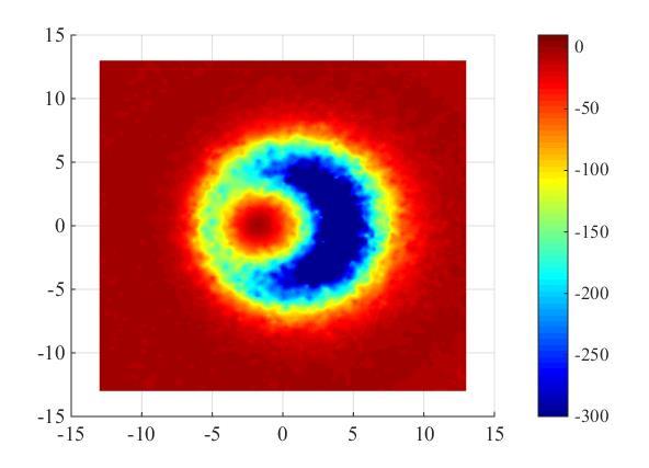
175 a b c 154