Joint inversion of crosshole radar and seismic traveltimes acquired at the South Oyster

Transcription

1 Joint inversion of crosshole radar and seismic traveltimes acquired at the South Oyster Bacterial Transport Site Niklas Linde 1, Ari Tryggvason 2, John Peterson 3, and Susan Hubbard 3 1 Swiss Federal Institute of Technology, Institute of Geophysics, Zurich, Switzerland; 2 Department of Earth Sciences/Geophysics, Uppsala University, Uppsala, Sweden; 3 Earth Sciences Division, Lawrence Berkeley National Laboratory, Berkeley, California, USA. Abstract: The structural approach to joint inversion, entailing common boundaries or gradients, offers a flexible way to invert diverse types of surface-based and/or crosshole geophysical data. The cross-gradients function has been introduced as a means to construct models in which spatial changes in two models are parallel or anti-parallel. Inversion methods that use such structural constraints also provide estimates of non-linear and non-unique field-scale relationships between model parameters. Here, we invert jointly crosshole radar and seismic traveltimes for structurally similar models using an iterative non-linear traveltime tomography algorithm. Application of the inversion scheme to synthetic data demonstrates that it better resolves lithological boundaries than the individual inversions. Tests of the scheme on observed radar and seismic data acquired within a shallow aquifer illustrate that the resultant models have improved correlations with flowmeter data than with models based on individual inversions. The highest correlation with the flowmeter data is obtained when the joint inversion is combined with a stochastic regularization operator, where the vertical integral scale is estimated from the flowmeter data. Point-spread functions shows that the most significant resolution improvements of the joint inversion is in the horizontal direction. 1

2 1. Introduction To determine petrophysical properties, state variables, and structural boundaries, it may be necessary to combine information provided by models obtained from different geophysical data (e.g., Tronicke et al., 2004; Bedrosian et al., 2007). Interpretation of several individually inverted data sets can be illuminating, but the results are usually affected by the resolution limitations of each model. For consistent interpretations of multiple geophysical models, it would be advantageous to have inversion tools that have similar formulations of the inverse problem regardless of the type of geophysical data being inverted. This would allow models to be coupled, as long as the data have comparable spatial support. By joint inversion, we refer to coupled models that are obtained by simultaneously minimizing a misfit function that includes the data misfit of each data type. Joint inversion can improve the resolution of each geophysical model and provide models that are consistent with each other and therefore easier to interpret (e.g., Gallardo and Meju, 2004). Joint inversion is not yet a standard tool in geophysical applications, mainly because robust and well-established petrophysical models that can be used to couple the models are usually only available for certain geophysical parameters, such as compressional and shear wave slownesses (Tryggvason et al., 2002). Furthermore, petrophysical models often apply only in restricted geological settings (e.g., Sen et al., 1981; Marion et al., 1992). In addition, the parameters of petrophysical models can seldom be adequately constrained by individual field data sets, such that fairly strong assumptions are required to couple models based on their petrophysical properties. To avoid introducing questionable petrophysical models, joint inversion methods have been developed for layered (1D) structures that are expected to have coincident layer boundaries and constant properties within each layer (e.g., Monteiro Santos et al., 2006). A 2

3 natural extension to two- and three-dimensional applications has been to assume that the earth can be divided into sub-volumes of uniform properties with geometries that are common for all physical properties in the inversion (e.g., Hyndman and Gorelick, 1996; Musil et al., 2003). Such approaches are certainly useful, but physical properties can vary gradually in space and not all data are necessarily sensitive to the same changes in lithology and state variables. Furthermore, the zonations must be updated continuously, making the inversions computationally expensive. In Occam s inversion (Constable et al., 1987), fine model discretizations are used and the inverse problem is regularized by minimizing, for example, model roughness with the constraint that the simulated model response is close to a given target data misfit. Haber and Oldenburg (1997) introduced a joint inversion scheme to find models that are structurally similar, in the sense that spatial changes in models occur at the same location. This scheme is applicable to over-parameterized two- and three-dimensional models and it is essentially based on minimizing the squared difference of a weighted Laplacian of the two models. Gallardo and Meju (2003) further developed the framework of the structural approach to joint inversion proposed by Haber and Oldenburg (1997) by defining the cross-gradients function t(x,y,z) as A B ( x y z) m ( x y z) m ( x y z) t,, =,,,,, (1) A B where m ( x, y, z) and m ( x, y, z) are the gradients of models m A and m B at location x, y, and z, and indicates the cross-product. By forcing the discretized cross-gradients function to be close to zero at each location during the inversion process, either the gradients of the two resulting models will be parallel or anti-parallel to each other or one or both of the models does not change. The boundaries of the resulting models have the same orientation, thus facilitating geological interpretations. An advantage compared to the work of Haber and Oldenburg (1997) is that constraints based on the cross-gradients function do not focus on the 3

4 magnitudes of the changes, which are difficult to estimate a priori and may necessitate a number of tuning parameters, but rather on a common direction. The validity of imposing the cross-gradients function to be zero is discussed by Linde et al. (2006a) in the context of electrical properties. The cross-gradients function was first employed in two-dimensions to invert jointly surface-based electrical resistance tomography (ERT) and seismic refraction profiles collected over weathered granodioritic bedrock overlain by mudstone (Gallardo and Meju, 2003; 2004). The same seismic refraction data was later jointly inverted with controlled-source audio magnetotelluric data (Gallardo and Meju, 2007). Recently, Gallardo (2007) proposed an extension of the cross-gradients function that allows the simultaneous inversion of more than two data types. Gallardo (2007) then used this scheme in two-dimensions to jointly invert surface-based P-wave and S-wave traveltimes, ERT, and magnetic data. Tryggvason and Linde (2006) presented the first three-dimensional application of joint inversion based on the cross-gradients function. By jointly inverting P- and S-wave traveltimes in a synthetic local earthquake tomography experiment, they found that the resulting anomalous V p /V s -ratios were better defined than those obtained by separate inversions or joint inversion based on damping the solution around a pre-defined V p /V s ratio. The efficiency of this approach was demonstrated on seismological data collected in the surroundings of the Hengill volcanic system on Iceland (Tryggvason and Linde, 2007). Linde et al. (2006a) jointly inverted crosshole ground penetrating radar (GPR) and ERT data collected in unsaturated sandstone in three dimensions. Scatter plots of the jointly inverted models were used together with petrophysical models to infer a zonation and to determine possible ranges of the electrical formation factors, water contents, and effective grain radius of the sediments within each of the zones. The resulting estimates were consistent with gamma logs, measured clay fraction, and electrical formation factor in a cored borehole. 4

5 Linde et al. (2006a) presented the only study so far in which geophysical models obtained from joint inversions using the cross-gradients function were evaluated against borehole data. However, their example provided by the unsaturated Sherwood Sandstone was limited by the one-dimensional character of the geology. We acknowledge that the crossgradients method needs to be applied to additional well-instrumented study sites before it is widely accepted. Here, we present the results of jointly invertied crosshole radar and seismic traveltimes recorded at the South Oyster study site, VA (Chen et al., 2001; Hubbard et al., 2001), where the geology consists of saturated unconsolidated sediments with three-dimensional heterogeneity. To guide the choice of inversion parameters, we calculate trade-off curves between the weight given to the cross-gradients constraint in the objective function and the resulting structural similarity of the resulting model, as well as between the weight given to the cross-gradients constraints and the weight given to the regularization operators. Finally, the improved resolution offered by the joint inversion is visualized with point-spare functions calculated in the central part of the interwell region. 2. Method 2.1 The inversion method Our formulation of the joint inverse problem closely follows that developed by Linde et al. (2006a) for use with ERT and GPR data. In the algorithm, the first arrival traveltimes are computed with the finite difference (FD) algorithm time3d (Podvin and Lecomte, 1991; Tryggvason and Bergman, 2006). Ray tracing is performed by a posteriori back propagation perpendicular to the wave fronts from the receivers to the transmitters (Hole, 1992). Our objective function have three competing components: the data fit resulting from two piece-wise constant individual slowness models m A and m B weighted by the estimated data errors; regularization of the individual models by penalizing model complexity (the relative 5

6 weights given to the regularization operators are determined by B ε and ε, where small Α p p values provides a strong relative weight); and coupling of the two models by enforcing structural similarity via cross-gradients constraints (the weight given to this term is controlled by λ). These objectives are formulated in one objective function that we seek to minimize, at each iteration, in a least-squares sense (see equations 8-9 in Linde et al. (2006a)) with the iterative conjugate gradient algorithm LSQR (Paige and Saunders, 1982). We regularize the inverse problem by seeking either a model that has small secondderivatives (i.e., smoothness constraints) or is close to a given stationary exponential covariance function. Linde et al. (2006a) show how such stochastic regularization operators can be calculated efficiently. To include the structural constraints in our objective function, we discretize the cross-gradients function, equation 1, with a central finite-difference scheme, which provides better results than the forward difference scheme used in previous work (e.g., Gallardo and Meju, 2004). The cross-gradients function for a candidate model is estimated using a first-order Taylor expansion around the cross-gradients function at the previous iteration (see equation 7 in Linde et al. (2006a)). 2.2 Inversion strategy The goal of the inversion is to construct two models where each model explain the data within pre-defined data errors (i.e., the weighted RMS of each of the models are very close to Α B 1) for a given λ, with the smallest possible value of ε p and ε p. For the joint inversion of radar and seismic traveltimes, in which the same type of traveltime tomography is employed and in which the relative variations in the model are expected to be similar, we assign ε = ε = ε. A simple way to test this assumption is to perform individual inversions to Α B p p p assure that ε Α p ε at the final iteration stage. When considering methods with significantly B p different resolution characteristics or relative variations in the parameters inverted for, we 6

7 Α B recommend to follow Linde et al. (2006a) and perform a line-search for both ε p and ε p at each iteration. To simplify the inversion process, we keep λ fixed during the inversion and choose it such that the objective function is dominated by the terms that force the linearized cross-gradients function to be close to zero. In Section 4.2, we investigate how the choice of λ affects the resulting model. The joint inverse problem is non-linear not only because the ray-paths depend on the slowness structure, but also because the cross-gradients function is non-linear (equation 1). The derivatives of the cross-gradients function are only valid in the vicinity of the previous model, and care must be made such that the updates are made within the region where the linearized cross-gradients function is reasonably valid. To avoid large model updates outside the region where the linearizations are valid, we keep ε p small in the first few iterations such that we solve a problem in which the regularization operator is heavily weighted relative to the data fit. This means that ε 1 is chosen such that the relative improvement in the data fit is only approximately 10%. In each iteration, we evaluate three candidate models derived from the inversion for 1/1.3 ε p, ε p, and 1.3 ε p, respectively. We retain the model with the lowest RMS, or the model with the smallest ε p that meets the target misfit. The trade-off parameter corresponding to the preferred model, will be the new ε p in the next iteration. When the target data misfit has been reached, we perform additional inversions where we seek to decrease ε p under the constraint that the resulting models explain the data within the target data misfit. These additional inversions where only minor changes between iterations occur, also serve the purpose of further decreasing the value of the cross-gradients function. This approach where we only gradually change ε p requires more inversion steps than a full line-search at each iteration (Linde et al., 2006a), but it allows the non-linearity of the cross-gradients function to be better accounted for. 7

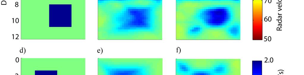
8 To visualize the results, we introduce a normalized cross-gradients function as B (,, ) (,, ) A m x y z m x y z t' ( x, y, z) =, (8) A B m m where the cross-gradients function is weighted by the absolute values of the models and where ( x, y, z) t' has units of m -2 regardless of the units of the inverted parameters. 3. Synthetic example A synthetic example is used to demonstrate the impact of the cross-gradients constraints on the solution of the inverse problem. Figure 1a shows a GPR velocity model that consists of three homogeneous rectangular zones of high- (100 m/µs) and low velocity (50 m/µs) embedded in a homogeneous background (75 m/µs). Figure 1d shows a matching seismic velocity model, where the high- and low velocities are 2 km/s and 1km/s, respectively, embedded in a homogeneous background of 1.5 km/s. A discretization of m 2 is used both for the forward and the inverse modeling yielding 1750 model cells for each model type. The two models are characterized by sharp boundaries that are difficult to resolve using individual smoothness-constrained inversions. These models illustrate a case in which the petrophysical relationships between the radar and seismic velocities are non-unique. Our synthetic experiment involved seismic and GPR pulses transmitted at intervals of 0.25 m in the m depth range of a borehole located along the left side of the model. The resulting traveltimes were computed in the high-frequency limit for a set of receivers with the same interval and depth range in a borehole located on the right side of the model. We restricted the inversions to the rays with angles less than 45. This is often done in field applications to avoid fast GPR ray-paths within the boreholes and because traveltime calculations are typically based on the assumption that the radar antenna acts like a point source, thereby overestimating velocities when inverting data with high angular 8

9 coverage. The traveltimes were contaminated with uncorrelated Gaussian noise with standard deviations of 0.5 ns and 20 µs for the radar and seismic traveltimes, respectively. The resulting radar and seismic velocity models of the individual inversions are shown in Figures 1b and 1e, respectively. The models are smeared, such that it is difficult to determine the actual geometry of the zones. The models also indicate that the locations of the highest velocities in the common high velocity zone differ for the seismic and radar models. The radar and seismic velocity estimates are plotted for every collocated model pair between the boreholes (Figure 2a). This scatter plot seems to indicate that the sub-surface is composed of three different anomalous zones. The resulting radar and seismic velocity models of the joint inversion are shown in Figures 1c and 1f, respectively. The three zones are less smeared out and the geometries of the upper and lower zones correspond well with the actual geometries. In addition, the common high-velocity zone in Figures 1c and 1f have fairly uniform velocities. The scatter plot in Figure 2b has very little scatter in the direction normal to the main axes of velocity gradients and the anomalies can therefore be picked by eye (for additional examples and discussions illustrating this, see Gallardo and Meju (2004, 2007), Linde et al. (2006a), Tryggvason and Linde (2006)). All models have a weighted RMS very close to one. As expected, the models constructed from the individual inversions and the joint inversion all resolve the high velocity zones better than the low velocity zones. Figure 2b indicates that the joint inversion resolves the upper zone of high seismic velocity better than the corresponding zone of low radar velocity, and vice versa for the lower zone where the radar velocity is high and the seismic velocity is low. However, the joint inversion greatly improves the geometry of the low velocity zones (e.g., compare the low velocity zone in Figure 2b with the one in Figure 2c). 9

10 The velocity contrasts considered in the example above are larger than the ones encountered in most environmental applications. Figure 2c and 2d shows the scatter plots resulting from individual inversions and joint inversion, respectively, for a model where the velocity range of the radar model was m/µs and km/s for the seismic model. The low velocity zones are now better resolved since the ray coverage in the low velocity regions is improved. 4. A field example We now consider radar and seismic traveltime data collected between wells S14 and M3 in the South Oyster Focus Area, Virginia (Hubbard et al., 2001). The radar data were collected using a PulseEKKO 100 system with 100 MHz nominal frequency antennas and a transmitter and receiver spacing of m in each borehole. The seismic data were collected using a Geometrics Strataview seismic system, a Lawrence Berkeley National Laboratory piezoelectric source, and an ITI hydrophone sensor string. The central frequency of the pulse was 4000 Hz, with a bandwidth from approximately 1000 to 7000 Hz, and the source and geophone spacings in the boreholes were m. These high-resolution data sets consist of 3248 radar and 2530 seismic traveltimes. We used a discretization of m 2 in our forward modeling, and a model discretization of m 2 for the inverse solution. We defined a target data misfit of 0.5 ns for the radar traveltimes and 20 µs for the seismic traveltimes. 4.1 Individual inversions The individual inversions were carried out using two different types of regularization: an anisotropic roughness operator that penalizes spatial variations in the horizontal direction five times as much as in the vertical direction, and a stochastic regularization operator (Linde et al., 2006a) based on an exponential model with a vertical integral scale of 0.28 m and an anisotropy factor of five, which is the model that was proposed and used by Hubbard et al. 10

11 (2001). The marine shore-face deposits at Oyster are expected to have a longer horizontal than vertical correlation length, such that assuming a certain anisotropy in the regularization provides geologically more reasonable models compared with isotropic regularization. The individually inverted smoothness-constrained radar (Figure 3a) and seismic (Figure 3e) velocity models contain a common low-velocity zone in the upper 2 m and a common high velocity zone at 4-5 m. The radar velocity model also includes a smaller low-velocity zone at 3 m, which is much less pronounced in the seismic model. The radar model includes a low velocity zone at m that is not seen in the seismic model, possibly because of low ray-coverage in that depth interval. A scatter plot of velocities presented by the two models indicates an overall positive relationship (Figure 3m) with a correlation coefficient of The individually inverted radar (Figure 3b) and seismic (Figure 3f) velocity models based on the stochastic regularization include the same main zones as those based on the smoothness-constrained inversions. However, the former models are more variable, since stochastic regularization operators represent a combination of general smoothness constraints (i.e., providing smooth models) and damping constraints (i.e., providing uncorrelated smallscale variability around an a priori model) (Maurer et al., 1998). The short vertical integral scale used here makes the zones thinner, more variable, and more pronounced. The models based on the stochastic regularization tend to split the upper low-velocity zones into two different horizontally aligned zones; a similar behavior is found in the high-velocity zone at 4-5 m. Again, a scatter plot of the radar and seismic velocities (Figure 3n) indicate a strong correlation with a correlation coefficient of Joint inversions A series of joint inversions with stochastic regularizations was carried out with different weights λ given to the cross-gradients constraints. Figure 4a indicates that the smallest value of the cross-gradients function is obtained for a λ of , which results in models where 11

12 the cross-gradients function is approximately 100 times smaller than for the individual inversions. Figure 4b shows that a λ in the range of 100 to enforces the trade-off parameter in the final iteration ε p to be increased with 30% compared with the individual inversions. As λ grows above , ε p is increased significantly to achieve a model that fit the target data misfit. The inversion results presented below were performed with a λ of , which corresponds to the structurally most similar models and where the spatial variability of the models are only slightly larger than those of the individual inversions. The models obtained by jointly inverting radar (Figure 3c) and seismic (Figure 3g) traveltimes with anisotropic smoothness constraints contain the same main zones as in the individually inverted models. However, the resolution is higher, since more small-scale variability is present and the boundaries between the different zones are sharper. The lowvelocity zone in the upper 2 m of the seismic model is divided into two. A high-velocity region between 2-3 m on the left side of the model, which is only weakly indicated in the individually inverted models, appears more clearly in the jointly inverted model. The highvelocity zone at 4 m becomes thinner and more elongated, and the modeled velocities are higher than those in the individually inverted models. Finally, the low-velocity zone at m in the radar velocity model now appears in the seismic model. The associated scatter plot (Figure 3o) are less scattered and thereby easier to interpret than those of the individually inverted models (Figures 3m and 3n). As expected, there is a strong positive correlation between the radar and seismic velocities, but there are also zones in which the relationship changes, thereby demonstrating the flexibility of the structural approach to joint inversion to deal with non-stationary apparent petrophysical relationships. The correlation coefficient is The models obtained by jointly inverted radar (Figure 3d) and seismic (Figure 3h) traveltimes with stochastic regularization operators are spatially the most variable, but they 12

13 contain mostly the same features as observed in models based on anisotropic smoothness constraints. The associated scatter plot (Figure 3p) indicates a strong linear correlation between the radar and seismic velocities, with a correlation coefficient of Table 1 demonstrates that the RMS data fit for all models are quite similar. The joint inversions decrease the scatter in the scatter plots significantly (Figures 3o and 3p), but they do not markedly change the trends that appear in the scatter plots for the individual inversions (Figures 3m and 3n). This indicates that also the regularization operator is very important, since it will significantly influence any zonation or petrophysical interpretation of the models. The visual similarity between the individual inversions and the joint inversions indicates that the joint inversion is not getting trapped in a local minima. 4.3 Image appraisal To investigate the resolution characteristics of the resulting models, we calculate the point-spread function (PSF) for the final inversion models based on the stochastic regularizations. The PSF is a row of the resolution matrix and it can be interpreted as the spatial averaging filter that relates the true underlying model to the resulting model estimate at a specific location. The PSFs are calculated with the LSQR algorithm analogously to the method presented by Alumbaugh and Newman (2000) for the conjugate gradient method and assuming that the cross-gradients function for the true model is zero. The PSFs based on the joint inversions are first normalized with regards to the mean values of the radar and seismic slownesses. The PSFs are then normalized with regards to the largest value in accordance with Alumbaugh and Newman (2000). Horizontal and vertical profiles through the normalized PSFs at a central location (depth=3.2 m, distance=3.4 m) are shown in Figure 5. As expected, the individual inversions have similar PSFs for the radar and seismic inversions. A much poorer horizontal (Figures 5a and 5c) than vertical resolution (Figures 5b and 5d) is evident. The profile of the PSF in the 13

14 horizontal direction is more narrow for the joint inversion (Figures 5a and 5c) than for the individual inversions indicating a higher resolution. In addition, the PSF constructed for the joint inversion has no side lobes in the vertical direction (Figures 5b and 5d). The radar model from the joint inversion is at this location only dependent on the surrounding radar estimates, and not of the seismic model (Figures 5a-5b). The seismic model is here primarily affected by the neighboring seismic estimates, but it is also strongly affected by the surrounding radar estimates. This observation can be explained when studying the models at this location. The radar model indicates a low velocity zone with a significant gradient that influences the resulting seismic model through the cross-gradients constraints (see equation 7 in Linde et al. (2006a)). The seismic model is fairly uniform at this location and do therefore not impose any significant restrictions on the radar model. The PSFs constructed for the joint inversion are thus strongly dependent on the neighboring values of the seismic and radar slowness models. This means that the PSFs are only meaningful if they are evaluated around the final model estimate. 4.4 Comparison with flowmeter data Hubbard et al. (2001) used tomograms from the Oyster site together with flowmeter data to create a hydraulic conductivity model. The flowmeter data collected in the boreholes were first kriged to provide a prior model of hydraulic conductivity. Relationships between geophysical attributes and hydraulic conductivity were developed using collocated tomographic estimates and flowmeter data; these relationships had a linear correlation coefficient of 0.68 (between hydraulic conductivity and radar velocity) and 0.67 (between hydraulic conductivity and seismic velocity). A Bayesian model was then used to update this prior model based on the observed correlation between flowmeter data and collocated geophysical estimates. Schiebe and Chien (2003) found that model predictions based on 14

15 stochastic indicator simulations conditioned to these estimates were superior to those based on stochastic indicator simulations conditioned to the flowmeter data alone. The usefulness or not of geophysical tomograms for constraining hydrological models is strongly dependent on the intrinsic relationships between the geophysical properties and hydraulic conductivity, here most likely through a common link with porosity (e.g., Carcione et al., 2007). If the models based on the joint inversions correlate better with the flowmeter data, it should be possible to improve the hydraulic conductivity model of Hubbard et al. (2001) and hence also solute transport predictions. To evaluate if the joint inversions are likely to provide better models than those supplied by the individual inversions, we have compared hydraulic conductivity estimates based on flowmeter data at borehole M3 (located near the right side of the tomographic models in Figure 3) with tomographic estimates located two model cells away from the borehole. The flowmeter data are shown in Figure 6a and the collocated radar velocity and seismic velocity models are shown in Figures 6b and 6c, respectively. To facilitate comparison, we highlight three depth intervals where the hydraulic conductivity data display a local minimum (Low 1-3) and three where they display a local maximum (High 1-3). The radar velocity model based on individual inversion with stochastic regularization accurately indicates five zones, whereas the radar model based on anisotropic smoothness constraints only accurately indicates one zone. The seismic velocity model based on stochastic regularization accurately indicates five zones, whereas the seismic model based on anisotropic smoothness constraints does not indicate any of these zones. The correlation coefficients of the collocated models based on the separate inversion and the flowmeter data are higher for the stochastic regularization (i.e., 0.72 for radar velocity and 0.60 for seismic velocity) than for the anisotropic smoothness constraints (i.e., 0.63 for radar velocity and 0.49 for seismic velocity). 15

16 The models based on the joint inversion with stochastic regularization indicate all six zones. The radar model based on the anisotropic regularization indicates three zones and the seismic velocity model indicates four zones. The correlation coefficients of the collocated models based on joint inversion and the flowmeter data are higher when using the stochastic regularization (i.e., 0.78 for radar velocity and 0.69 for seismic velocity) than when using the anisotropic smoothness constraints (i.e., 0.67 for radar velocity and 0.52 for seismic velocity). These results are summarized in Table 2 and they indicate that joint inversion with stochastic regularization at this site offer higher resolution and accuracy in determining lithological changes than the other inversion approaches considered here. Stochastic regularization operators based on borehole data (flowmeter data) provided better models than those supplied by traditional anisotropic smoothness constraints. Indeed, changes associated with varying the regularization operator seem to improve the resulting models slightly more than the joint inversion. The radar and seismic traveltime data could not individually provide the necessary resolution to image the small-scale variability revealed by the flowmeter data. Regularization based on flowmeter data from the site and the assumption that the two models are structurally similar improves the resolution of the resulting models. 5. Discussion The resulting inversion models are qualitatively similar and they reach the target misfit for all inversion types considered. This indicates that the non-linearity of the cross-gradients function do not cause the joint inversion process to be trapped in local minima for the examples considered here. When performing this type of joint inversion, we recommend to first perform individual inversions to assess if the models appear to be structurally similar. In addition, the individual inversions help to define a target data misfit and to assure that ε Α p ε. The joint inversion is expected to focus the images obtained from the individual B p inversions. If the joint and individual inversion models are very different, this is likely to 16

17 indicate that the two physical properties under consideration are not structurally similar or that the model updates at the early iteration steps have been too large. The best way to choose λ when performing the joint inversions is to perform a series of inversions with different choices of λ (see Figure 4). The resolution improvements offered by the joint inversion vary from case to case and throughout the model domain since it is largely dependent on the spatial variations of the physical parameters inverted for. To evaluate the resolution improvements, we recommend to calculate PSFs at selected locations (see Figure 5) as suggested by Alumbaugh and Newman (2000). We expect that some of the oscillations in the horizontal profiles of the PSF (e.g., Figure 5c) is caused by the discretization of the cross-gradients constraints, which operates on neighboring model cells only. This problem could be avoided if the cross-gradients constraints were discretized on the same scale as the stochastic regularization operator. The stochastic regularization operator defines a presumably known scale on which structure is resolved. Large integral scales will result in large-scale features with large amplitudes, small integral scales will result in a heavily damped solution with a lot of smallscale variability (see Maurer et al. (1998) for a good illustration). This implies that the magnitudes exhibited in the scatter plots of radar and seismic velocities (e.g., Figure 3p) are dependent on the regulartization operator. The synthetic example also shows that earth models with large variability (e.g., Figure 1a and 1d) will introduce bias in the resulting scatter plots (see Figure 2b), since the velocity of low-velocity zones will be over-estimated. These effects must be considered when making petrophysical interferences from such scatter plots (e.g., Linde et al., 2006a). The sharper boundaries and the more variable models offered by the joint inversion with stochastic regularization are likely to significantly improve flow- and transport predictions if used to constrain hydrological model compared with using individually inverted models with 17

18 smoothness constraints. In the future, we plan to develop new strategies to infer the underlying geometry and physical properties of earth model from jointly inverted models. The resulting method will be used to parameterize a three-dimensional flow- and transport model at an ongoing research site. 6. Conclusions The structural approach to joint inversion is based on the assumption that the two relevant physical properties have common structural boundaries. Gallardo and Meju (2003) introduce a quantitative measure of structural similarity that they term the cross-gradients function. By discretizating and linearizating the cross-gradients function, it is possible to define a joint inversion method that penalizes models where the gradients of two models are neither parallel nor anti-parallel. We use the cross-gradients function to develop an iterative non-linear traveltime tomography algorithm that jointly inverts seismic and GPR traveltimes. A synthetic example shows that the joint inversion improves the determination of the boundaries of three anomalous zones as well as their geometry compared with models based on individual inversions. The inversion method was applied to crosshole radar and seismic traveltime data collected in an unconsolidated and saturated environment. The inverse problem was regularized (i) with an exponential geostatistical model based on flowmeter data and tomographic estimates presented in Hubbard et al. (2001) and (ii) with anisotropic smoothness constraints. The radar and seismic velocity models based on individual inversions indicated a strong structural similarity, in which the models based on stochastic regularization showed more variability for a given data misfit. The magnitudes of the cross-gradients function for the models based on the joint inversion were approximately 1% of the individually inverted models. The jointly inverted models were not only structurally more similar, but they also displayed larger spatial variability for a given data fit. 18

19 We used flowmeter data collected in one of the boreholes to assess if the stochastic regularization and the joint inversion could improve the resulting models as indicators of geological variability. We identified three zones in which the flowmeter data indicated local minima in the hydraulic conductivity and three zones indicating local maxima. The joint inversion based on the stochastic regularization was the only one that accurately located all six zones. Since tomographic models may be used to constrain hydrological flow and transport models (e.g., Hubbard et al., 2001; Schiebe and Chien, 2003; Linde et al., 2006b), we suggest that if structural similarity can be established, then the structural approach to joint inversion and the use of borehole data to determine the regularization operators has the potential to improve such hydrological models. Acknowledgments We thank Alan Green and Stewart Greenhalgh for commenting on draft versions of this manuscript. We also thank the Associate Editor, Lanbo Liu, and three anonymous reviewers for construcive reviews that helped to improve the paper. Funding for this study was partially provided by the Environmental Remediation Science Program, Office of Biological and Environmental Research, U.S. Department of Energy Grant DE-AC02-05CH

20 References Alumbaugh, D. L., and G. A. Newman, 2000, Image appraisal for 2-D and 3-D electromagnetic inversion: Geophysics, 65(2), Bedrosian, P. A., N. Maercklin, U. Weckmann, Y. Bartov, T. Ryberg, and O. Ritter, 2007, Lithology-derived structure classification from the joint interpretation of magnetotelluric and seismic models: Geophysical Journal International, 170(2), doi: /j x x Carcione, J. M., B. Ursin, and J. I. Nordskag, 2007, Cross-property relations between electrical conductivity and the seismic velocity of rocks: Geophysics, 72(5), E193-E204. Chen, J., S. Hubbard, and Y. Rubin, 2001, Estimating the hydraulic conductivity at the South Oyster Site from geophysical tomographic data using Bayesian techniques based on the normal linear regression model: Water Resources Research, 37(6), Constable, S. C., R. L. Parker, and C. G. Constable, 1987, Occam s inversion: a practical algorithm for generating smooth models from EM sounding data: Geophysics, 52(3), Gallardo, L. A., and M. A. Meju, 2003, Characterization of heterogeneous near-surface materials by joint 2D inversion of dc resistivity and seismic data: Geophysical Research Letters, 30(13), doi: /2003gl Gallardo, L. A., and M. A. Meju, 2004, Joint two-dimensional DC resistivity and seismic travel time inversion with cross-gradient constraints: Journal of Geophysical Research, 109, B03311, doi: /2003JB Gallardo, L. A., 2007, Multiple cross-gradient joint inversion for geospectral imaging, Geophysical Research Letters, 34, L19301, doi: /2007GL Gallardo, L. A., and M. A. Meju, 2007, Joint two-dimensional cross-gradient imaging of magnetotelluric and seismic traveltime data for structural and lithological classification: 20

21 Geophysical Journal International, 169(3), doi: /j X x Haber, E., and D. Oldenburg, 1997, Joint inversion: A structural approach: Inverse problems, 13(1), Hole, J. A., 1992, Nonlinear high-resolution three-dimensional seismic travel time tomography: Journal of Geophysical Research, 97(B5), Hyndman, D. W., and S. M. Gorelick, 1996, Estimating lithological and transport properties in three dimensions using seismic and tracer data: the Kesterson aquifer: Water Resources Research, 32(9), Hubbard, S. S., J. Chen, J. Peterson, E. L. Mayer, K. H. Williams, D. J. Swift, B. Mailloux, and Y. Rubin, 2001, Hydrogeological characterization of the South Oyster Bacterial Transport Site using geophysical data: Water Resources Research, 37 (10), Linde, N., A. Binley, A. Tryggvason, L. B. Pedersen, and A. Revil, 2006a, Improved hydrogeophysical characterization using joint inversion of crosshole electrical resistance and ground penetrating radar traveltime data, Water Resources Research, 42, W doi: /2006wr Linde, N., S. Finsterle, and S. Hubbard, 2006b, Inversion of tracer test data using tomographic constraints: Water Resources Research, 42, W doi: /2004wr Maurer, H., K. Holliger, and D. E. Boerner, 1998, Stochastic regularization: Smoothness or similarity?: Geophysical Research Letters, 25(15), Marion, D., A. Nur, H. Yin, and D. Han, 1992, Compressional velocity and porosity in sandclay mixtures: Geophysics, 57 (4), Monteiro Santos, F. A., S. A. Sultan, P. Represesas, and A. L. El Sorady, 2006, Joint inversion of gravity and geoelectrical data for groundwater and structural investigation: 21

22 applicatiom to the northwestern part of Sinai, Egypt: Geophysical Journal International, 165, doi: /j X x Musil, M., H. R. Maurer, and A. G. Green, 2003, Discrete tomography and joint inversion for loosely connected or unconnected physical properties: application to crosshole seismic and georadar data sets: Geophysical Journal International, 153(2), Paige, C. C., and M. A. Saunders, 1982, LSQR: An algorithm for sparse linear equations and sparse least squares: ACM Transactions on Mathematical Software, 8(1), Podvin, P., and I. Lecomte, 1991, Finite difference computation of travel times in very contrasted velocity models: A massively parallel approach and its associated tools: Geophysical Journal International, 105(1), Scheibe, T. D., and Y. J. Chien, 2003, An evaluation of conditioning data for solute transport prediction: Ground Water, 41, Sen, P. N., C. Scala, and M. H. Cohen, 1981, A self-similar model for sedimentary-rocks with application to the dielectric-constant of fused glass-beads: Geophysics, 46(5), Tronicke, J., K. Holliger, W. Barrash, and M. D. Knoll, 2004, Multivariate analysis of crosshole georadar velocity and attenuation tomograms for aquifer zonation: Water Resources Research, 40, W doi: /2003wr Tryggvason, A., S. Th. Rögnvaldsson, and Ó. G. Flovenz, 2002, Three-dimensional imaging of the P- and S-wave velocity structure and earthquake locations beneath Southwest Iceland: Geophysical Journal International, 151(3), Tryggvason, A., and B. Bergman, 2006, A travel time reciprocity inaccuracy in the time3d finite difference algorithm by Podvin & Lecomte: Geophysical Journal Intenational, 165(2), Doi: /j X x 22

23 Tryggvason, A., and N. Linde, 2006, Local earthquake (LE) tomography with joint inversion for P- and S-wave velocities using structural constraints: Geophysical Research Letters, 33, L doi: /2005gl Tryggvason, A. and N. Linde, 2007, Local earthquake tomography for P- and S-velocity structure using 3D cross-gradients constraints: 69 th Conference & Exhibition, EAGE, Expanded Abstracts, June. 23

24 Figure captions Figure 1. (a, d) True radar and seismic velocity models; (b,e) individually inverted radar and seismic velocity models; (c, f) jointly inverted radar and seismic velocity models. Figure 2. (a) and (b) Scatter plots of the individually and jointly inverted models shown in Figure 1, respectively. The large dots in (a) and (b) are the true velocity values and the small dots with the same color coding are ranges of the tomographic estimates at the corresponding locations. (c) and (d) Corresponding scatter plots where the true velocity values have a smaller range as indicated by the large dots. Figure 3. Radar velocity models from Oyster: (a) individual inversion with anisotropic smoothness constraints, (b) individual inversion with stochastic regularization, (c) joint inversion with anisotropic smoothness constraints, (d) joint inversion with stochastic regularization, (e) to (h) corresponding seismic velocity inversion results, (i) to (l) the cross-gradients function for these models, (m) to (p) scatter plots of these models. Figure 4. (a) The mean value of t and (b) ε p for different choices of λ. The values correspond to those of the final iteration of the inversion with stochastic regularization operators. Figure 5. (a, d) Normalized PSFs of the final radar models in the horizontal and the vertical direction and (c, d) for the corresponding seismic models. Dotted line indicates profiles of PSFs from the individual inversions with stochastic regularization, solid line indicates PSFs of radar parameters for joint inversion with stochastic regularization and the dashed line indicates the corresponding seismic parameters. Figure 6. (a) Flowmeter data of hydraulic conductivity in borehole M3 (located on the right side of the tomograms in Figure 3); (b) tomographic radar velocity models two model cells away from M3; (c) tomographic seismic velocity models two model cells away from M3. The red solid and dotted line in (b-c) represent models from the joint inversion model 24

25 with stochastic regularization and anisotropic smoothness constraints, respectively; the black solid and dotted lines represent the corresponding models for the individual inversions. The zones (Low 1-3) are locations where the measured hydraulic conductivity has a local minima and the zones (High 1-3) where it has a local maxima. Table 1. Final RMS value with regards to a target data fit of 0.5 ns for the radar traveltimes and 20 µs for the seismic traveltimes. The data fits for all inversions are practically the same. Table 2. The table indicates to what extent low (Low 1-3) and high (High 1-3) permeability zones can be identified in the different inversion models. The correlation coefficients (ρ) between the flowmeter data and collocated inversion models are also summarized. 25

26 26

27 27

28 28

29 29

30 30

31 31

32 Inversion type RMS of Radar model RMS of seismic model Individual inversion, anisotropic smoothness constraints Individual inversion, stochastic regularization Joint inversion, anistropic smoothness constraints Joint inversion, stochastic regularization

33 Separate inversions Joint inversions Radar models Seismic models Radar models Seismic models smooth stochastic smooth stochastic smooth stochastic smooth stochastic Low High Low High Low High ρ