GEOCLIMATIC DESIGN OF WATER BALANCE COVERS FOR MUNICIPAL SOLID WASTE LANDFILLS IN TEXAS

Transcription

1 January 20, 2017 GEOCLIMATIC DESIGN OF WATER BALANCE COVERS FOR MUNICIPAL SOLID WASTE LANDFILLS IN TEXAS TXSWANA WATER BALANCE STUDY TXSWANA has not thoroughly reviewed this study, but has noted a discrepancy between the cover thickness recommended in the DFW area and other nearby areas, and recommends that additional study be undertaken before this study is relied upon for use in designing covers in Texas. Board of Directors Lone Star Chapter of the Solid Waste Association of North America (TXSWANA)

2

3 TABLE OF CONTENTS ACKNOWLEDGEMENT... 8 EXECUTIVE SUMMARY INTRODUCTION DESIGN APPROACH METEOROLOGICAL DATA Precipitation Data Solar Radiation Data Modeled vs. Measured Dataset Modeled Dataset PET Estimates GEOCLIMATIC REGIONS SOIL TESTING WATER BALANCE MODELING Central Texas Field-Scale Water Balance Study Conceptual Model Soil Properties Meteorological Data Vegetation Data Initial Conditions and Numerical Control Parameters WATER BALANCE COVER DESIGNS In-Service Hydraulic Conductivity In-Service vs. As-Built Hydraulic Conductivities IMPLEMENTATION AND CONSTRUCTION QA/QC POST-CLOSURE MONITORING APPLICABILITY AND ASSUMPTIONS REFERENCES APPENDIX A: UNSAT-H INPUT FILES APPENDIX B: AVERAGE ANNUAL PERCOLATION PREDICTED BY UNSAT-H APPENDIX C: AVERAGE ANNUAL RUNOFF PREDICTED BY UNSAT-H 2

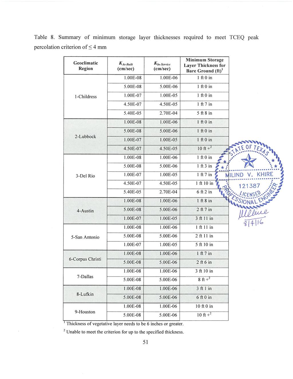
4 APPENDIX D: AVERAGE ANNUAL ET PREDICTED BY UNSAT-H LIST OF TABLES Table 1. Precipitation and PET/P for weather stations located in Texas Table 2. PET/P for Geoclimatic Regions for APY and WPY Table 3. Summary of geotechnical properties for samples collected from the geoclimatic regions Table 4. Fitting parameters for soil-water characteristic curves Table 5. Fitting parameters for unsaturated hydraulic conductivity functions Table 6. Yearly weather parameters for geoclimatic regions for average precipitation year Table 7. Yearly weather parameters for geoclimatic regions for wet precipitation year Table 8. Summary of minimum storage layer thicknesses required to meet TCEQ peak percolation criterion of 4 mm

5 LIST OF FIGURES Figure 1. Average annual precipitation contours for Texas obtained from 50 years of historic data Figure 2. Wet year annual precipitation contours for Texas obtained from 50 years of historic data Figure versus 96.7 percentile annual precipitation for Texas weather stations Figure 4. Contours of PET/P for average precipitation year Figure 5. Contours of PET/P for wet precipitation year Figure 6. Comparison of APY and WPY potential evapotranspiration (PET) for Texas weather stations Figure 7. Delineated Geoclimatic regions for Texas with average year annual precipitation contours Figure 8. Delineated Geoclimatic regions for Texas with wet year annual precipitation contours Figure 9. Soil sampling locations Figure 10. Saturated hydraulic conductivity vs. molding water content with respect to OMC Figure 11. Saturated hydraulic conductivity vs. finer fractiona Figure 12. Instrumented lower catchment during early Spring 2012 after a year of drought Figure 13. Measured precipitation and runoffs from upper and lower catchments Figure 14. Cumulative runoff to cumulative precipitation ratio during the monitoring period Figure 15. Measured runoff versus runoff simulated by UNSAT-H for upper catchment Figure 16. Measured runoff versus runoff simulated by UNSAT-H for lower catchment Figure 17. Conceptual model of water balance cover for UNSAT-H modeling Figure 18. Peak annual percolation predicted by UNSAT-H vs. thickness of storage layer for inservice storage layer hydraulic conductivity of 10-6 cm/s

6 Figure 19. Peak annual percolation predicted by UNSAT-H vs. thickness of storage layer for inservice storage layer hydraulic conductivity of cm/s Figure 20. Peak annual percolation predicted by UNSAT-H vs. thickness of storage layer for inservice storage layer hydraulic conductivity of 10-5 cm/s Figure 21. Peak annual percolation predicted by UNSAT-H vs. thickness of storage layer for inservice storage layer hydraulic conductivity of cm/s Figure 22. Peak annual percolation predicted by UNSAT-H vs. thickness of storage layer for inservice storage layer hydraulic conductivity of cm/s Figure 23. Required minimum storage layer thickness vs. in-service saturated hydraulic conductivity of the storage layer Figure 24. Relationship between as-built and in-service hydraulic conductivities Figure 25. Required minimum storage layer thickness vs. as-built saturated hydraulic conductivity of the storage layer

7 LIST OF SYMBOLS AND ABBREVIATIONS = van Genuchten soil-water characteristic curve fitting parameter dmax = maximum dry unit weight r = residual volumetric water content s = saturated volumetric water content = matric suction = gravimetric water content opt = optimum gravimetric water content cm = centimeter (unit of length) cm/s = centimeter per second (unit of speed) ft = feet (unit of length) hr = hour (unit of time) in = inch K( ) = unsaturated hydraulic conductivity of soil at soil suction of K In-service = in-service saturated hydraulic conductivity K As-built = as-built saturated hydraulic conductivity K sat = saturated hydraulic conductivity l = van Genuchten Maulem pore-interaction parameter m = van Genuchten soil-water characteristic curve fitting parameter n = van Genuchten soil-water characteristic curve fitting parameter pcf = pound per cubic feet (unit of unit weight) sec = seconds (unit of time) APY = Average precipitation year 6

8 ET = Evapotranspiration NOAA = National Oceanic and Atmospheric Administration NCDC = National Climatic Data Center NREL = National Renewable Energy Laboratory NSRDB = National Solar Radiation Data Base OMC = Optimum moisture content P = Precipitation PET = Potential evapotranspiration PET/P = Ratio of potential evapotranspiration to precipitation SWCC = Soil-water characteristic curve TCEQ = Texas Commission on Environmental Quality TxSWANA = The Lone Star Chapter of the Solid Waste Association of North America UHCF = Unsaturated hydraulic conductivity function UNSAT-H = Unsaturated Flow and Heat Flow Model USCS = Unified Soil Classification System WB = Water balance WPY = Wet precipitation year 7

9 ACKNOWLEDGEMENT Texas Commission on Environmental Quality (TCEQ) Waste Permits Division brought together stakeholders representing public and privately owned solid waste landfills to fund this project. Earl Lott of TCEQ organized several conference calls and meetings over the duration of this project. Dwight Russell of TCEQ spent invaluable amount of time as he provided his regulatory input throughout the duration of the project. TCEQ s efforts are appreciated. Several key stakeholders including Mike Caldwell, Vance Kemler, Holly Holder, Scott Trebus, and Wade Wheatley provided valuable practical input during various phases of this project and also provided soil samples for testing and characterization. This project was initially funded at Michigan State University (MSU) and later transferred to the University of North Carolina, Charlotte. These graduate students assisted in the laboratory and field testing and computer modeling phases of this project: Tryambak Kaushik and Tula Ngasala. Waste Management, Inc. funded the catchment-scale surface runoff monitoring project at the Austin Community Landfill. Mike Caldwell, Terry Johnson, and the site staff at Austin Community Landfill provided valuable support for this long-term field water balance cover project. The data collected from this project was used to validate the runoff estimation capabilities of UNSAT-H for an in-service water balance cover. 8

10 EXECUTIVE SUMMARY This report represents the work product of a joint effort between stakeholders represented by the TCEQ Office of Waste, Waste Permits Division, the Lone Star Chapter of TxSWANA representing both public and privately owned solid waste landfills, and the University of North Carolina, Charlotte. The intended purpose of this report is to summarize the findings of numerical water balance modeling for ten geoclimatic regions in Texas with the outcome of a series of template water balance cover designs based on climate and soil type. The intent of these designs is to provide final cover designs that can be approved for construction and meet the requirements for equivalency without the need to construct field verification test plots or additional modeling by the owner/operator of MSW landfills located in 9 of the total 10 geoclimatic regions. The scope of work included the designation of ten (10) geoclimatic regions primarily based on PET/P ratio, annual precipitation, and the locations of weather stations with high quality and comprehensive meteorological data obtained from National Climatic Data Center. Soil samples were collected from seven geoclimatic regions and submitted for laboratory analysis of grain size, moisture-density evaluation, and saturated hydraulic conductivity testing. In-service saturated and unsaturated hydraulic properties were estimated or adapted from published long-term field-scale studies. Transpiration was not simulated due to lack of regionspecific data needed for modeling water balance covers. The collected and available data were input into UNSAT-H for numerical modeling based upon guidance for cover performance metrics provided by TCEQ in the technical guide entitled Guidance for Requesting a Water Balance Alternative Final Cover for a Municipal Solid Waste Landfill (TCEQ RG-494), dated January Partial validation of UNSAT-H model was carried out with a field-scale multiyear water balance study at an in-service water balance final cover located in central Texas. The final cover designs that meet the TCEQ performance criteria are presented in a chart in this report. These designs can be used by the owners of the solid waste landfills when seeking approval for a water balance cover once site-specific borrow soils are characterized. The minimum borrow soil characterization required includes laboratory analysis of grain size, moisture-density relationships, and saturated hydraulic conductivities as a function of compaction effort and molding water content. 9

11 1 INTRODUCTION Based on the scope of work submitted to the Lone Star Chapter of the Solid Waste Association of North America (TxSWANA) in October 2012 and a revised scope submitted in December 2013, this report presents the geoclimatic region-specific design of water balance covers for solid waste landfills located in Texas. This scope was reviewed and approved by the Texas Commission on Environmental Quality (TCEQ). This project was commissioned by TxSWANA with the primary goal being that geoclimatic region-specific designs developed in this project would offer another option for TCEQ to issue permits to the stakeholders for alternative or water balance final covers for Type 1 landfills located in Texas without a need to construct field verification test plots or additional modeling. The water balance covers were designed to meet the TCEQ design criteria stated in the water balance (WB) cover guidance document Guidance for Requesting a Water Balance Alternative Final Cover for a Municipal Solid Waste Landfill (TCEQ RG-494), dated January 2012 (TCEQ 2012). The guidance document allows for an alternative final cover if it achieves an equivalent reduction in percolation and equivalent protection from wind and water erosion as the prescriptive or conventional geomembrane cover. The scope of this design document was limited to the design of water balance covers using numerical modeling carried out using the water balance model UNSAT-H (Fayer and Jones 1990, Fayer 2000). The water balance cover guidance document (TCEQ 2012) requires a WB cover modeling and design process to demonstrate that the simulated percolation at the bottom of the WB final cover is 4 mm for each of the years during a consecutive 30-year period of record. TCEQ (2012) allows 8 mm annual percolation if verification testing is carried out. However, geoclimatic-region specific designs may not need to be verified in the field. Hence, annual percolation 4 mm was used as the criterion to design geoclimatic region-specific water balance covers. The scope of the designs presented in this report is strictly limited to hydrologic or water balance modeling that relates to the percolation criterion. The design of water balance covers to meet the wind or water erosion criteria was not part of the scope. In addition, slope stability analysis, design of a stormwater management system, or equivalency analysis with a conventional cover were not part of the scope. 10

12 2 DESIGN APPROACH The approach followed to design geoclimatic region-specific water balance covers consisted of: 1. Obtaining long-term comprehensive meteorological data as required by the model UNSAT-H for 24 weather stations located in Texas where this data as required by UNSAT-H has been measured; 2. Using the meteorological data to estimate potential evapotranspiration (PET) for each of the 24 locations of the weather stations; 3. Using the spatial distribution of PET and other variables to divide Texas into representative geoclimatic regions; 4. Measuring region-specific soil properties consisting of soil classification, moisturedensity relationships and saturated hydraulic conductivities to identify the soil groups that might be used as final covers; and 5. Using published field-scale unsaturated hydraulic properties of various types of soils coupled with long-term meteorological data to design region-specific water balance covers that meet the TCEQ (2012) percolation criterion. 3 METEOROLOGICAL DATA Meteorological data is an integral part of water balance modeling and establishing a representative climate for each region to ascertain long-term site-specific performance of water balance covers. It is not unusual for long-term hydrologic modeling to become limited in scope and prediction due to lack of high-quality meteorological data. The National Climatic Data Center (NCDC) database ( managed by the National Oceanic and Atmospheric Administration (NOAA) was reviewed and 24 Texas weather stations were identified where comprehensive meteorological data consisting of daily values of precipitation, maximum and minimum air temperatures, average relative humidity (or dew point), average wind speed and total solar radiation. A majority of these identified stations had about 50 years of recorded (or simulated data for solar radiation) data. The 50 years of climate data obtained and analyzed for the water balance modeling ranged from 1961 to

13 3.1 Precipitation Data A total of 31 stations in Texas were identified with at least 50 consecutive years of precipitation data. Two climate years, namely average precipitation year (APY) and wet precipitation year (WPY) were identified for each station in Texas. An APY received 50 percentile 50-year annual precipitation, while a WPY received 95 percentile annual precipitation. The years with missing rainfall data were not used in the evaluation of average or 95 percentile precipitation. A summary of annual precipitation based on at least 50 years of data at all identified stations in Texas is presented in Table 1. Figs. 1 and 2 show the contour maps of average and wet year precipitation. While all 31 stations were used to draw precipitation contours, Figs. 1 and 2 only show the 24 comprehensive weather data stations. Fig. 2 shows that there are relatively high annual precipitation contours just to the north of Del Rio. This precipitation data was obtained for weather station located in Carta Valley (Item 25 in Table 1). 3.2 Solar Radiation Data The National Renewable Energy Laboratory (NREL) provides access to the national solar radiation database (NSRDB) (Wilcox 2012). The database contains 1,454 stations across the United States, with 89 stations in Texas Modeled vs. Measured Dataset The NSRDB has measured solar radiation data for 40 stations across the nation with 8 stations located in Texas for a limited number of years. The NSRDB provides modeled solar radiation data at hourly intervals in a dataset from 1961 forward. METSTAT (Maxwell 1998) software was used by the NSRDB to model solar radiation with measured input parameters such as solar radiation data (global, direct, and diffuse radiation), dry bulb temperature, dew-point temperature, humidity, wind speed, aerosol optical depth, precipitation, and atmospheric pressure. 12

14 Serial Number Table 1. Precipitation and PET/P for weather stations located in Texas Station NSRDB Class APY Precipitation (in) PET/P for APY WPY Precipitation (in) PET/P for WPY 1 Abilene I Austin I Brownsville I Corpus Christi I Dallas I Houston I Lubbock I Lufkin I Midland I Port Arthur I San Angelo I San Antonio I Victoria I Waco I Amarillo I Childress II Cotulla II Dalhart II Del Rio II Laredo II Wichita Falls II Texarkana II Longview II College Station II Carta Valley Menard Rocksprings Brackettville Camp Wood Sonora APY is average precipitation year. 2. WPY is wet precipitation year. 13

15 Legend * Weather Station Type1 Landfill Average Annual Precipitation (in) Figure 1. Average annual precipitation contours for Texas obtained from 50 years of historic data 14

16 Legend * Weather Station Type1 Landfill Wet Year Annual Precipitation (in) Figure 2. Wet year annual precipitation contours for Texas obtained from 50 years of historic data 15

17 3.2.2 Modeled Dataset Because, measured solar radiation data is only for a limited number of years and for relatively few stations in Texas, modeled solar radiation data were used in this project. The modeled NSRDB data is available in two sets: 1. The old data set from ; and 2. The new data set from The new data set from 1991 to 2010 was used in this project. The old data set from 1961 to 1990 was not used due to the following limitations: 1. The old data set uses manual cloud cover observations while the new data set uses automated observations. Automated observations have relatively few data gaps compared to manual observations. 2. The old data set uses estimated aerosol, water vapor and ozone data as compared to measured aerosol, water vapor and ozone data in the new data set. 3. The new data set has a better quality controlled measured solar radiation data set and advanced satellite-based techniques to measure irradiance from the last two decades. 4. Classification of stations based on modeled data quality is available only for the new data set. The NSRDB classifies modeled solar radiation data in the new data set in three classes of stations as follows. 1. Class I. These stations are identified with a complete period of records for key meteorological fields and the highest quality of modeled solar radiation data. Texas has 15 Class I stations. All Class I stations were used for the data required to model water balance covers in this study. 2. Class II. These stations have a complete period of record but significant periods of interpolated, filled, or otherwise lower-quality input data for the solar models. A total of 9 Class II stations were identified in Texas for the current analysis. 16

18 3. Class III. These stations did not have complete measured records with a minimum of only three years of measured data available. Data from none of the class III stations was used in this study. 3.3 PET Estimates The Penman (1940) method incorporated in the UNSAT-H model (Fayer 2000) is commonly used to evaluate potential evapotranspiration (PET) demand for water balance covers (Khire et al. 1997; Khire et al. 1999; Khire et al. 2000; and Mijares and Khire 2012). 24 weather stations located in Texas had comprehensive long-term (1991 onwards) meteorological data available to estimate PET using the Penman method. The wet precipitation year had precipitation that exceeded the 95 percentile precipitation calculated from the 50-year record. 95 percentile precipitation corresponds to a wet year that repeats on average every 20 years. TCEQ water balance criterion (TCEQ 2012) requires modeling 30 consecutive years of meteorological data. However, due to the limited availability of high-quality solar radiation data, wet year data corresponding to 95 percentile precipitation was considered appropriate. Fig. 3 shows a plot of the 95 percentile (1 in 20 years) vs. the percentile (1 in 30 years) annual precipitation for all 24 weather stations in Texas. The difference in 95 percentile and percentile precipitation is relatively small (average ~ 6%) for all weather stations except Lufkin (~ 20%). PET was estimated for the 24 locations for APY and WPY using the Penman method. Table 1 presents the ratios of PET to precipitation (P) for the 24 weather stations. In addition, contour plots of PET/P are presented in Figs. 4 and 5 for APY and WPY, respectively. Figure 6 shows that PET is usually lower during wet years compared to average precipitation years. This shows that it is critical to use all climatic parameters collected during the specific years for which the water balance modeling is carried out. 4 GEOCLIMATIC REGIONS A total of 10 Geoclimatic regions were delineated based on these considerations: 1. Spatial distribution of PET/P; 2. Annual precipitation; 17

19 3. Relative magnitudes of percolation for identical designs; 4. County boundaries; and 5. Locations of weather stations with high-quality and comprehensive meteorological data; PET/P was the primary indicator used to delineate geoclimatic regions. The PET/P ratio was mapped based on PET/P estimated for the weather station locations for APY and WPY (Figs. 4 and 5). The PET /P ratio for Texas ranged from 1.1 to 7.5 for APYs and from 0.7 to 4.6 for WPYs. Generally, PET/P 1.0 is an indicator that a water balance cover with a relatively small percolation criterion (few mm per year) is not feasible due to lack of adequate evapotranspiration (ET) to remove stored water from the cover. The design thickness of a water balance cover is primarily influenced by the wet-year precipitation and the PET/P for the wet year (Kaushik 2014). Table 2 presents PET/P for APY and WPY for the 10 geoclimatic regions presented in Figs. 7 and 8. The regional PET/P presented in Table 2 reflect the arithmetic mean of PET/P of all weather stations located within the region that were included in the modeling. All boundaries of the geoclimatic regions were lined up with the boundaries of the counties or the state boundary (Figs. 7 and 8). 18

20 El Paso Midland Dalhart Amarillo Del Rio San Angelo Lubbock Childress Abilene Wichita Falls Cotulla Laredo Brownsville San Antonio Waco Corpus Christi Austin Dallas College Station Texarkana Longview Houston Victoria Lufkin Port Arthur Annual Precipitation (in) Percentile Precipitation Percentile Precipitation Figure vsersus 96.7 percentile annual precipitation for Texas weather stations 19

21 Legend PET/P < > 5.0 Figure 4. Contours of PET/P for average precipitation year 20

22 Legend PET/P < > 5.0 Figure 5. Contours of PET/P for wet precipitation year 21

23 El Paso Lubbock Midland Amarillo Dalhart Childress San Angelo Laredo Abilene Brownsville Wichita Falls Corpus Christi Dallas Waco Del Rio San Antonio Austin College Station Cotulla Victoria Longview Houston Port Arthur Texarkana Lufkin Annual PET (in) 125 Average Precipitation Year Wet Precipitation Year Figure 6. Comparison of APY and WPY potential evapotranspiration (PET) for Texas weather stations 22

24 Table 2. PET/P for Geoclimatic Regions for APY and WPY Geoclimatic Region Average Precipitation Year (APY) PET/P Wet Precipitation Year (WPY) PET/P 1. Childress Lubbock Del Rio Austin San Antonio Corpus Christi Dallas Lufkin Houston Port Arthur

25 Legend * Type1 Landfill Average Year Annual Precipitation (in) Figure 7. Delineated Geoclimatic regions for Texas with average year annual precipitation contours 24

26 Legend * Type1 Landfill Wet Year Annual Precipitation (in) Figure 8. Delineated Geoclimatic regions for Texas with wet year annual precipitation contours 25

27 Table 2 shows that for Region 1, PET/P ratio ranges from 2.5 to 4 and it ranges from 2.5 to 5 for Region 2 for WPY. The name of the region corresponds to the name of the location of the weather station within that region which was used to represent the weather for the entire region. Whenever possible, a weather station located centrally in that region was chosen. Simulated percolation not only depends on the PET/P and annual P but also on other parameters including distribution and intensity of storm events. While PET/P range and annual P for Regions 1 and 2 are about the same, preliminary water balance simulations using UNSAT-H indicated that Lubbock had greater percolation than any of the locations in Region 1. Hence, Lubbock was assigned as a separate region. Similarly, while PET/P range and P for Regions 4, 5, and 6 is about the same, preliminary water balance simulations using UNSAT-H indicated that San Antonio had greater percolation than Austin and Corpus Christi had less percolation than San Antonio but greater percolation than Austin. As a result, San Antonio and Corpus Christi were assigned as separate regions. Houston and Lufkin have similar PET/P and annual P. However, preliminary water balance simulations indicated that Lufkin had less percolation than Houston for identical water balance cover designs. Therefore, Lufkin was assigned as a separate geoclimatic region. Geoclimatic region 10 (Port Arthur) is located in the far eastern portion of Texas. A majority of this region has PET/P 1.0 for WPY. This region was considered too wet for a single layer water balance cover to be feasible. Consequently, this region was excluded in this study. Multilayer alternative covers consisting of lateral drainage layer(s), hydraulic storage layer(s), and/or hydraulic barrier layer(s) maybe feasible for this region. However, this evaluation was beyond the scope for this project. 5 SOIL TESTING Soil samples were collected from all geoclimatic regions except Regions 1 and 5. The soil samples were collected from one or two Type 1 landfill sites selected from each geoclimatic region. A total of 10 soil samples were collected and tested. The approximate locations of the sites where these samples were collected are presented in Fig. 9. Bulk soil samples were collected from borrow areas of the sites. 26

28 Figure 9. Soil sampling locations 27

29 TRI Environmental, Inc. was engaged by the site owners or operators to carry out the following tests: 1. USCS soil classification (ASTM D 2487); 2. Standard Proctor compaction (ASTM D 698); 3. Modified Proctor compaction (ASTM D 1557); 4. Specific gravity (ASTM D 854); and 5. Saturated hydraulic conductivity using flexible wall permeameter (ASTM D 5084). The key objective of carrying out these tests was to evaluate the range of saturated hydraulic conductivities that can be achieved for a range of compaction efforts and molding water contents for the geoclimatic regions. Saturated hydraulic conductivity is a key design parameter that influences the design thickness of a water balance cover. The Proctor compaction results were used to establish the dry of optimum moisture content (OMC) range for each of the sampled soils. For the saturated hydraulic conductivity tests, two samples were tested for each of the compaction efforts, one at the OMC and the other at 3 to 4% dry of OMC. The reason for testing the soils at dry of OMCs was to ensure relatively small structural changes in the compacted cover during service. Soils compacted dry of optimum undergo a smaller increase in saturated hydraulic conductivity during service because its shrink/swell potential is less than when it is compacted wet of optimum. Table 3 presents a summary of all geotechnical properties that were measured for the 10 soil samples collected in this project. Fig. 10 shows the saturated hydraulic conductivity as a function of molding water content relative to OMC. The hydraulic conductivity is generally higher when the soil is compacted at water contents drier than OMC. However, it is absolutely a requirement to compact the soil in the field at dry of OMCs for covers. Fig. 10 shows that the lowest lab-scale saturated hydraulic conductivity achieved was about 10-8 cm/s. One sample had saturated hydraulic conductivity that was in the 10-9 cm/s order, only when the sample was compacted relatively close to the OMC. When the sample was compacted at 4% dry of OMC, the saturated hydraulic conductivity was about 10-8 cm/s. Hence it was assumed that 10-8 cm/s is a practical lowest limit of as-built lab-scale saturated hydraulic conductivity for natural compacted soils in Texas. 28

30 Fig. 11 shows the saturated hydraulic conductivity as a function of the finer fraction ( 5 m). Based on the results for the 10 soils tested in this project, there is rapid decrease in the hydraulic conductivity as the finer fraction increases from 20% to 40%. For finer fraction ranging from 40% to 90%, there is insignificant influence on the hydraulic conductivity. Thus, it is expected that soils having finer fraction 40% will most likely yield the lowest hydraulic conductivities. 29

31 Table 3. Summary of geotechnical properties for samples collected from the geoclimatic regions. Geoclimatic Region 2-Lubbock 3-Del Rio 4-Austin 6-Corpus Christi 7-Dallas 8-Lufkin 9-Houston Location City of Lubbock Landfill City of Midland Ponderosa Regional Landfill Austin Community Landfill 1 City of Brownsville Cefe F. Valenzuela Landfill City of Denton Landfill City of Nacogdoches Landfill Ft. Bend Regional Landfill McCarty Road Landfill USCS Classification Not Provided SC Not Provided CH Not Provided CH CL SC CH CL Proctor Compaction Effort dmax (pcf) opt (%) (%) Hydraulic Conductivity 1 Deviation from opt K sat (cm/sec) Standard E E-05 Modified E E-06 Standard E E-05 Modified E E-06 Standard E E-07 Modified E E-08 Standard E-07 Modified E-08 Standard Modified Standard Modified Standard Modified Standard Modified Standard Modified Standard Modified > 0 is dry of optimum, = 0 is at optimum, and < 0 is wet of optimum E E E E E E E E E E E E E E E E E E E E E E E E E E E E-07 30

32 Saturated Hydraulic Conductivity (cm/sec) Houston Lufkin Corpus Christi Dallas Austin Del Rio Lubbock Open Symbol: Standard Proctor Closed Symbol: Modified Proctor OMC: Optimum Moisture Content Wet of optimum Dry of optimum Gravimetric Water Content: OMC-Molding (%) Figure 10. Saturated hydraulic conductivity vs. molding water content with respect to OMC 31

33 Saturated Hydraulic Conductivity (cm/sec) Lubbock Del Rio Austin Dallas Corpus Christi Houston Closed Symbol: Modified Proctor Open Symbol: Standard Proctor Fraction Finer than 5 m (%) Figure 11. Saturated hydraulic conductivity vs. finer fraction 32

34 6 WATER BALANCE MODELING Water balance modeling was carried out using the public domain finite-difference water balance model UNSAT-H Ver (Fayer 2000). Each of the 9 geoclimatic regions with all possible soil types that could be used in that region to design a WB cover that will meet the TCEQ percolation criterion (TCEQ 2012) was modeled. Use of UNSAT-H or another approved equivalent model for water balance modeling is one of the design requirements in the TCEQ guidance document (TCEQ 2012). UNSAT-H has been validated in several field studies since the early 1990s (Fayer and Jones 1990; Khire et al. 1997; Benson et al. 2005; Mijares and Khire 2012). UNSAT-H numerically solves a modified form of Richards equation to calculate the flow of water through both saturated and unsaturated soil(s). UNSAT-H can simulate water and heat flow processes in one dimension (1-D) and is capable of simulating steady-state and transient conditions. UNSAT-H does not simulate flow through macropores because they do not follow capillarity and hence cannot be represented by Richards equation. UNSAT-H also does not consider air/gas pressures. Therefore, if air/gas pressures develop during rapid infiltration events, the model is unable to simulate the flow accurately. However, natural infiltration events in compacted fine-grained soils do not develop air or gas pressures due to relatively slow moving wetting fronts. 6.1 Central Texas Field-Scale Water Balance Study In a recent catchment-scale study carried out at the Austin Community Landfill (ACL), which is a Type I landfill located in Austin, Texas, UNSAT-H was validated using catchment scale runoff measured at two instrumented catchments of a 3-acre portion of the water balance cover that has been in service for over 6 years (Kaushik 2014; Kaushik et al. 2014). ACL is located in Geoclimatic Region 4. At ACL the monitoring system was designed to measure surface runoff and soil water contents and suction. The cover consisted of 3-ft thick compacted native clay overlain by 0.5-ft thick topsoil to support vegetation. The landfill cover is sloped at 1V to 4H. The compacted clay is high plasticity clay (CH) according to the Unified Soil Classification System (USCS) and was designed to function as the soil water storage layer. The 33

35 clay was compacted in lifts to achieve 95% relative compaction at the Standard Proctor effort at up to 5% wet of the optimum moisture content. Two adjacent catchments were instrumented to measure surface runoff and soil water contents. The upper catchment was 100 ft 400 ft (0.9 acres) while the lower catchment was 175 ft 400 ft (1.6 acres). A berm approximately 1 ft high, separated surface water runoff from the upper and lower catchments. Runoff monitoring system was installed in December 2011 when the vegetation on the cover was relatively scant due to drought in 2011 (Fig. 12). Three nests consisting of four water content and matric suction sensors each were installed within the two catchments to estimate in-situ unsaturated hydraulic properties of the cover. Total precipitation received during the monitoring period Dec 2011 to Nov 2013 was 70 in. The potential evapotranspiration (PET) to precipitation ratio (PET/P) for the monitored period was 2.1. A total of 132 storms were recorded and 29 storms produced runoff. ACL received an average precipitation of 0.1 in/hr for all precipitation events over the monitoring period. The upper catchment shed 8.25 in (12% of precipitation) runoff and the lower catchment shed 5.5 in (8% of precipitation) runoff during the monitoring period (Fig. 13). The upper catchment recorded a maximum event runoff of 1.9 in (from a 2.6 in precipitation event), a minimum event runoff of 2.7E-3 in (from a 0.55 in precipitation event), and an average event runoff of 0.28 in for the rainfall events generating runoff during the monitoring period. The lower catchment recorded a maximum event runoff of 1.4 in (from a 2.6 in precipitation event), a minimum event runoff of 7.9E-4 in (from a 0.55 in precipitation event), and an average event runoff of 0.2 in for the rainfall events generating runoff during the monitoring period. While the cumulative runoff averaged 12% and 8% of annual precipitation over the 23 month monitoring period for the two catchments, it varied significantly throughout the period. Cumulative runoff for the upper and lower catchments peaked at 22.5% and 17% in April 2012, and decreased to a minimum of 7.6% and 5.5% in September 2013, respectively (Fig. 14). However, cumulative runoff gained in the following months and finally ended at 12% and 8% for upper and lower catchments, respectively, in November Density of vegetation, antecedent moisture contents, PET/P, and duration, intensity and magnitudes of storms were the key variables that may have influenced the magnitude of runoff. 34

36 Cumulative Runoff (in) Figure 12. Instrumented lower catchment during early Spring 2012 after a year of drought 100 Precipitation 10 Upper Catchment (12%) Lower Catchment (8%) Dec/15 Apr/15 Aug/15 Dec/15 Apr/15 Aug/ Figure 13. Measured precipitation and runoffs from upper and lower catchments 35

37 Cumulative Runoff Cumulative Precipitation (%) Upper Catchment 10 5 Lower Catchment 0 Dec/15 Apr/15 Aug/15 Dec/15 Apr/15 Aug/ Figure 14. Cumulative runoff to cumulative precipitation ratio during the monitoring period Kaushik (2014) numerically modeled both catchments using the numerical water balance models UNSAT-H and the Root Zone Water Quality Model (RZWQM) using meteorological and soil hydraulic properties measured in the field. The field-based unsaturated hydraulic properties of the cover were estimated using data collected from sensors embedded in the cover in the field using the method used by Mijares & Khire (2012). RZWQM over-estimated the runoff by a factor of two and UNSAT-H underestimated runoff for one of the two instrumented catchments by about 50% while it slightly underestimated runoff for the second instrumented catchment. Kaushik (2014) demonstrated by additional modeling that with a slight decrease in the input value of the saturated hydraulic conductivity of the vegetative layer (topsoil layer), the model was able to predict the runoff very accurately. This shows that hydrology of water balance covers is very sensitive to the in-service hydraulic properties of the soils that constitute the cover. Hence, input of representative in-service hydraulic conductivities is vital for accurate predictions. Figures 15 and 16 show the runoff simulated by UNSAT-H when the surface layer hydraulic conductivity was corrected such that field and simulated runoffs are relatively close. 36

38 Cumulative Runoff (in) Cumulative Runoff (in) 5 Upper Catchment 4 Measured 3 2 UNSAT-H 1 0 Dec/15 Mar/15 Jun/15 Sep/15 Dec/15 Mar/ Figure 15. Measured runoff versus runoff simulated by UNSAT-H for upper catchment 4 Lower Catchment 3 Measured 2 UNSAT-H 1 0 Dec/15 Mar/15 Jun/15 Sep/15 Dec/15 Mar/ Figure 16. Measured runoff versus runoff simulated by UNSAT-H for lower catchment 37

39 6.2 Conceptual Model A schematic of the conceptual model used for modeling each of the water balance covers is presented in Fig. 17. The model consisted of a 6-inch thick vegetative or topsoil layer underlain by a storage layer. The underlying waste was not modeled. Mijares and Khire (2012) demonstrated that the underlying waste, which exists in the field application, acts as a temporary storage layer for infiltration which can be partially removed via ET. Therefore, ignoring the underlying waste would usually yield conservative values of percolation. If a waste layer is modeled, site-specific waste properties are required and generically assuming waste properties may result in erroneous predictions. Hence, waste layer was not modeled. The thickness of the storage layer was varied from 1 ft to 8 ft for a majority of simulations. Relatively few simulations were carried out with storage layer thickness of 10 ft. The thinnest storage layer was assumed to be 1-foot thick because, in the author s opinion, that is the practical limit to construct a compacted soil layer in the field that can maintain its physical integrity during construction and service. The maximum thickness of 8 ft was selected based on economic considerations. The upper boundary of the model was specified as a variable flux boundary. The variable flux boundary corresponds to the infiltration rate if it is raining during a given time period or evaporation rate if otherwise. The lower boundary was simulated as unit gradient boundary. Figure 17. Conceptual model of water balance cover for UNSAT-H modeling 38

40 6.3 Soil Properties The soil properties input to UNSAT-H consisted of albedo, saturated hydraulic conductivity, and fitting parameters for soil-water characteristic curves (SWCCs) and unsaturated hydraulic conductivity functions (UHCFs). The albedo value that was input to the model for all simulations was 0.2. This value has been used by Khire et al. (1997), Mijares and Khire (2012), and Kaushik (2014) in the field validation studies of UNSAT-H. Tables 4 and 5 summarize the unsaturated hydraulic parameters input to UNSAT-H. The SWCCs are described by the van Genuchten (1980) function (Table 4) and the unsaturated hydraulic conductivities are described by the van Genuchten-Mualem (1976) function (Table 5). The van Genuchten function (van Genuchten 1980) is as follows (Eq. 1): s r 1 r n m (1) where = matric suction head; = water content; s = saturated water content; r = residual water content; and, n, and m (m =1-n -1 ) are fitting parameters. Table 4. Fitting parameters for soil-water characteristic curves Parameter r (-) s (-) (1/cm) n (-) Source CH Soil Kaushik et al. (2014) ML-CL/SC Soil Khire and Gromachenko (2014) SM-ML Soil Khire et al. (2000) SM-ML Soil Khire et al. (1997) SM Soil Khire et al. (2000) Vegetative Layer Kaushik et al. (2014) The unsaturated hydraulic functions were described by Mualem (Mualem 1976) function to predict the unsaturated hydraulic conductivities using the van Genuchten fitting parameters 39

41 and the saturated hydraulic conductivities. The van Genuchten-Mualem model (Mualem 1976) is as follows (Eq. 2): nm n m 1 ( ) [1 ( ) ] 2 K( ) K sat [1 ( ) n ] ml (2) where K sat is saturated hydraulic conductivity; K( ) is unsaturated hydraulic conductivity at matric suction ; and l is pore-interaction term. Table 5. Fitting parameters for unsaturated hydraulic conductivity functions Parameter K sat (cm/sec) (1/cm) n (-) l (-) Source CH Soil Kaushik et al. (2014) ML-CL/SC Soil Khire and Gromachenko (2014) SM-ML Soil Khire et al. (2000) SM-ML Soil Khire et al. (1997) SM Soil Khire et al. (2000) Vegetative Layer Kaushik et al. (2014) In this project, unsaturated properties for the CH soil were obtained from a water balance cover that has been in service in Austin. The unsaturated hydraulic properties were not measured for other soil samples. However, lab-scale saturated hydraulic conductivities were measured. Mijares and Khire (2012) have demonstrated that lab-scale unsaturated hydraulic properties are not representative for simulating water balance of covers in the field. A majority of unsaturated hydraulic properties presented in Tables 4 and 5 were obtained from the water contents and soil suctions measured in the field for instrumented test sections of covers. Hence, these hydraulic properties are representative of hydraulic properties of covers in service. 40

42 The saturated hydraulic conductivities input to UNSAT-H represent the long-term saturated hydraulic conductivities of the vegetative layer and the storage layers for covers in service. The as-built hydraulic conductivities are required to be up to two orders of magnitude less than the in-service saturated hydraulic conductivities to account for pedogenesis. Pedogenesis is formation of cracks and preferential flow paths due to desiccation, freeze-thaw and plant root intrusion (Benson et al. 2007). The as-built saturated hydraulic conductivities and their relationship with in-service saturated hydraulic conductivities is explained in Section Meteorological Data Each of the 9 geoclimatic regions was represented by a NOAA weather station that is located within the region. Each of the weather stations had historical records ( 20 years) of daily values of: precipitation, maximum and minimum air temperatures, average relative humidity (or dew point), average wind speed, and total solar radiation. The geoclimatic regions and the representative weather stations are listed in Tables 6 and 7. Tables 6 and 7 also list a summary of weather parameters for the selected average and wet precipitation years, respectively. UNSAT-H requires geographic parameters and daily values of weather parameters presented in Tables 6 and 7 to estimate potential evapotranspiration and evaporation. UNSAT-H allows input of daily or hourly values of precipitation. Hourly values of precipitation are not available for all weather stations. Kaushik (2014) carried out sensitivity of daily versus hourly precipitation values on runoff predictions for Austin. Kaushik (2014) observed a difference of less than 1% in predicted runoffs. In this project, because hourly precipitation values were not available for all the selected years for all weather stations, in order to maintain consistency, only daily precipitation values were used. 41

43 Table 6. Yearly weather parameters for geoclimatic regions for average precipitation year Average Precipitation Year Geoclimatic Region No. Weather Station Latitude ( N) Altitude (ft) Precipitation (in) Daily Solar Radiation (Wh/m 2 ) Daily Temperature ( F) Daily Dew Point Temperature ( F) Daily Wind Speed (miles/hr) 1 Childress 34 1, to to to 71 3 to 30 2 Lubbock 34 3, to to to 69 4 to 25 3 Del Rio to to to 72 3 to 18 4 Austin to to to 76 2 to San Antonio to to to 75 2 to 16 Corpus Christi to to to 78 4 to 25 7 Dallas to to to 74 2 to 25 8 Lufkin to to to 78 1 to 15 9 Houston to to to 77 2 to 16 42

44 Table 7. Yearly weather parameters for geoclimatic regions for wet precipitation year Wet Precipitation Year Geoclimatic Region No. Weather Station Latitude ( N) Altitude (ft) Precipitation (in) Daily Solar Radiation (Wh/m 2 ) Daily Temperature ( F) Daily Dew Point Temperature ( F) Daily Wind Speed (miles/hr) 1 Childress 34 1, to to to 71 4 to 25 2 Lubbock 34 3, to to to 67 4 to 29 3 Del Rio to to to 75 1 to 21 4 Austin to to to 75 2 to San Antonio to to to 75 3 to 20 Corpus Christi to to to 79 3 to 23 7 Dallas to to to 74 3 to 24 8 Lufkin to to 98 8 to 77 1 to 14 9 Houston to to to 76 2 to 17 43

45 6.5 Vegetation Data UNSAT-H allows simulation of transpiration by plants when the following transpiration related parameters are input: (1) Root length density function; (2) maximum root depth; (3) growing season; (4) leaf area index (LAI); and (5) suctions that control the rate of water uptake by plants. While growing season and LAI of native grasses, shrubs, and other crops are well published for Texas, the root length density functions, maximum root depth and suctions that control the rate of water uptake by plants are site-specific parameters and there is very little data available that is applicable for Texas water balance covers. These parameters are expected to be influenced by location, soil type, density of the soil (dependent on level of compaction), plant type, and magnitude of seasonal precipitation. While plants are expected to remove water by transpiration, plants will develop preferential flow paths due to root intrusion and root decay (Melchior 1997; Wieler and Naef 2003; Khire and Saravanathiiban 2013) which adds to an unknown complexity in model input. UNSAT-H does not simulate preferential or macropore flow. In order to consider plants and simulate transpiration for water balance covers, site-specific measurements need to be carried out. Due to lack of such data, transpiration was not simulated. Nevertheless, plants are expected to be maintained to minimize erosion and to maintain aesthetics. A 0.5 ft thick vegetative soil layer that will support plants was simulated. 6.6 Initial Conditions and Numerical Control Parameters The modeling approach consisted of simulating 20 years of average precipitation year followed by one year of the wet year. This approach allowed prediction of percolation for a given water balance cover design for a return period of 20 years for the wet year selected with 95 percentile precipitation. The peak percolation values simulated by UNSAT-H during this 21-year simulation period were used to design the water balance cover that meets the TCEQ percolation criterion (TCEQ 2012). While the TCEQ requirement (TCEQ 2012) is to simulate 30 years of consecutive data, the 20-year return period allowed the use of high-quality and comprehensive weather data consistently for all weather stations that were selected to represent the 10 geoclimatic regions. In addition, Fig. 3 indicates that a wet year with a 30-year return period (96.7 percentile) has incrementally higher annual precipitation than a wet year with a 20-year 44

46 return period. As additional high-quality and comprehensive weather data becomes available in the future, the model results can be updated, if necessary. Initial conditions for UNSAT-H were specified across the depth of the soil profile by specifying matric suctions. The matric suctions corresponding to water contents at 60% degree of saturation were input to represent the initial conditions. 60% of degree of saturation is a representative degree of saturation when a cover is compacted at dry of optimum water contents. Spatial discretization of the model domain was optimized by conducting sensitivity analysis. This was done by repeatedly refining the nodal spacing until insignificant changes in simulated water balance parameters were achieved. The nodal spacing between the nodes located near the upper and lower boundaries, as well as near the interface between layers, was relatively small (~1 mm). The maximum spacing between the adjacent nodes ranged from 0.1 cm to 10 cm. A maximum time step of 1 hr and a minimum time step of hr were used for the simulations. This was necessary to accurately evaluate the extreme drying and wetting conditions typically encountered at the ground surface. For most numerical simulations, the mass balance error was less than 0.1 % of annual precipitation. All key input files prepared for all 9 geoclimatic regions for average as well as wet precipitation years are presented in Appendix A. 7 WATER BALANCE COVER DESIGNS Design of water balance covers was carried out by simulating various thicknesses of the storage layer using each of the 5 soil types listed in Table 4. These soil types represent finegrained to coarser-grained soils that can be used to design water balance covers in Texas. The thickness of the uppermost layer, the vegetative layer, was maintained fixed at 0.5 ft. A sensitivity analysis was carried out by increasing the vegetative layer thickness to 1 ft. Due to the relatively high hydraulic conductivity of the vegetative layer, insignificant decrease or no decrease in percolation was observed when the thickness was increased from 0.5 ft to 1 ft. The relatively high hydraulic conductivity of the vegetative layer represents the in-service hydraulic conductivity. It is relative high due to repeated volume changes of the surface layer from wetting and drying and intrusion of plant roots (Mijares and Khire 2012; Khire et al. 1999). 45

47 The storage layer thickness was increased from 1 ft to a value that resulted in peak annual percolation of 4 mm during the 21-year simulation period. For certain soil types in certain regions, an increase in storage layer thickness did not result in a significant decrease in peak annual percolation. In such cases, the maximum simulated thickness of the storage layer was limited to 8 ft to 10 ft for practicality. 7.1 In-Service Hydraulic Conductivity Figs. 18 to 22 present the peak annual percolation vs. the thickness of the storage layer for all geoclimatic regions for each of the storage layer soils presented in Tables 4 or 5. Appendix B presents the annual percolation predicted by UNSAT-H vs. thickness of storage layer for an average precipitation year. If a site owner or operator decides to use the design option which allows the owner to construct, instrument, and monitor a lysimeter for a proposed water balance cover design (TCEQ 2012), the plots presented in Appendix B will be useful to design as well assess performance of the cover during the monitoring period when annual precipitation may be less than 95 percentile precipitation corresponding to WPY. If the field measured annual percolation is greater than that presented in Appendix B for average precipitation year(s), there is a reasonable likelihood that the cover will not meet the TCEQ (2012) 4 mm annual peak percolation criterion if wet year precipitation were to occur during the monitoring period. Regional maps of predicted annual surface runoff and ET normalized with respect to precipitation for APY and WPY are presented in Appendices C and D, respectively. The annual runoff and ET are presented to provide region-specific as well as state-wide simulated water balance which can used as a guidance if water balance modeling were to be carried out using site-specific data when regional-scale design presented in this report may not be representative of the site conditions. Fig. 18 presents the peak annual percolation predicted by UNSAT-H vs. thickness of the storage layer for in-service storage layer hydraulic conductivity of 10-6 cm/s for the wet precipitation year. Except for Corpus Christi region, the wet precipitation year represents the year when simulated percolation peaked during the 21-year simulation period. For Corpus 46

48 Christi region, simulated percolation peaked for average precipitation year. The minimum thickness of the storage layer to achieve the TCEQ percolation criterion ranged from 1 ft for Childress, Lubbock, and Del Rio regions to 2.5 ft, 4 ft, and 10 ft for Lufkin, Dallas, and Houston regions, respectively. Fig. 19 presents the peak annual percolation predicted by UNSAT-H vs. thickness of storage layer for in-service storage layer hydraulic conductivity of cm/s for the wet precipitation year. Except for Corpus Christi region, the wet precipitation year represents the year when simulated percolation peaked during the 21-year simulation period. For Corpus Christi region, simulated percolation peaked for average precipitation year. The minimum thickness of the storage layer to achieve the TCEQ percolation criterion ranged from 1 ft for Lubbock region to 2.5 ft, 5 ft, and 6.5 ft for San Antonio, Lufkin, and Dallas regions, respectively. For the Houston region, the TCEQ percolation criterion was not achievable for storage layer thickness 10 ft. Fig. 20 presents the peak annual percolation predicted by UNSAT-H vs. thickness of storage layer for in-service storage layer hydraulic conductivity of 10-5 cm/s for the wet precipitation year. Except for Corpus Christi region, the wet precipitation year represents the year when simulated percolation peaked during the 21-year simulation period. For Corpus Christi region, simulated percolation peaked for average precipitation year. The minimum thickness of the storage layer to achieve the TCEQ percolation criterion ranged from 1 ft for Childress and Lubbock regions to 4 ft and 5 ft for Austin and San Antonio regions, respectively. For Dallas, Lufkin, and Houston regions, the TCEQ percolation criterion was not achievable for simulated storage layer thickness 10 ft. The required minimum storage layer thicknesses to achieve the TCEQ criterion are summarized in Table 8. 47

49 Peak Annual Percolation (mm/yr) 4 mm 100 K In-Service = 10-6 cm/s K As-Built = 10-8 cm/s Wet Precipitation Year 10 Houston 1 Austin Dallas Lufkin Note: Del Rio Corpus Christi 1 1 Peak percolation occurs in average precipitation year. 0.1 Childress San Antonio Lubbock Thickness of Storage Layer (ft) Figure 18. Peak annual percolation predicted by UNSAT-H vs. thickness of storage layer for inservice storage layer hydraulic conductivity of 10-6 cm/s. 48

50 Peak Annual Percolation (mm/yr) 4 mm 100 K In-Service = cm/s K As-Built = cm/s Wet Precipitation Year 10 Dallas Lufkin 1 Lubbock & Childress Del Rio Austin San Antonio Corpus Christi 1 Note: Peak percolation occurs during average precipitation year Thickness of Storage Layer (ft) Figure 19. Peak annual percolation predicted by UNSAT-H vs. thickness of storage layer for inservice storage layer hydraulic conductivity of cm/s. 49

51 Peak Annual Percolation (mm/yr) 4 mm Dallas Lubbock Lufkin K = 10-5 cm/s In-Service K = 10-7 cm/s As-Built Wet Precipitation Year Houston Corpus Christi 1 San Antonio 1 Childress Austin 0.1 Note: 1 Peak percolation occurs during average precipitation year. Del Rio Thickness of Storage Layer (ft) Figure 20. Peak annual percolation predicted by UNSAT-H vs. thickness of storage layer for inservice storage layer hydraulic conductivity of 10-5 cm/s. 50

52