SPATIAL ECOLOGY OF LARGE HERBIVORES IN THE SERENGETI ECOSYSTEM

Transcription

1 SPATIAL ECOLOGY OF LARGE HERBIVORES IN THE SERENGETI ECOSYSTEM By SMRITI BHOTIKA A DISSERTATION PRESENTED TO THE GRADUATE SCHOOL OF THE UNIVERSITY OF FLORIDA IN PARTIAL FULFILLMENT OF THE REQUIREMENTS FOR THE DEGREE OF DOCTOR OF PHILOSOPHY UNIVERSITY OF FLORIDA

2 2012 Smriti Bhotika 2

3 ACKNOWLEDGMENTS I thank my advisor, Robert Holt, and the members of my supervisory committee, Benjamin Bolker, Michael Binford, Todd Palmer, and Mary Christman, for the insights, guidance, and suggestions they offered on various aspects of my research, the contributions they made to my intellectual growth during my years of study, and the steadfast support and encouragement they provided throughout the process of completing this degree. I thank the National Center for Ecological Analysis and Synthesis (NCEAS) Serengeti Biocomplexity Working Group for making data for this project available and Tony Sinclair, Kris Metzger, and Grant Hopcraft for facilitating access to data sources. The Tanzania Wildlife Research Institute (TAWIRI), the Tanzania Wildlife Conservation Monitoring Program, and the Frankfurt Zoological Society provided animal survey data and maps of roads and rivers for the study area; S.J. McNaughton provided nutrient data; Rico Holdo provided nutrient maps; and J. Dempewolf provided fire maps. For awarding funds for this research, I thank the Harold Hume Presidential Fellowship, John Olowo Memorial Research Award, Department of Biology, School of Natural Resources and Environment, Center for African Studies, and the Office of Research and Graduate Programs of the University of Florida. I thank the faculty, staff, and graduate students in the department; their collegiality greatly influenced my journey in this degree program. In particular, Mike Barfield, Rico Holdo, and Kristen Sauby provided input, guidance, and encouragement during various stages of my research. I extend a special thanks to my dear friend Jame McCray, for her company during numerous work sessions and for her support week after week during the final stages of my graduate program. Lastly, my foundation -- I 3

4 thank my family and friends for believing in me and my parents for supporting me however and whenever they could throughout my lifetime and especially during this endeavor. 4

5 TABLE OF CONTENTS page ACKNOWLEDGMENTS... 3 LIST OF TABLES... 8 LIST OF FIGURES ABSTRACT CHAPTER 1 INTRODUCTION General Introduction Study Area Outline ON THE RELATIONSHIP OF A COMMUNITY OF LARGE HERBIVORES TO ENVIRONMENTAL AND ANTHROPOGENIC INFLUENCES IN THE SERENGETI ECOSYSTEM: A COMPARISON OF FOUR COMMUNITY MEASURES Methods Study Area Census Data Habitat Characteristics Statistical Analyses Community correlations Collinearity among habitat variables Spatial regression model selection Results Community Correlation Patterns Community Distribution Patterns Spatial Regression Model Selection Model Results Discussion Community Correlation Patterns Community Distribution Patterns Human activity Topography Resources Concluding Remarks OCCUPANCY AND ABUNDANCE PATTERNS IN RELATION TO SPECIES TRAITS FOR LARGE HERBIVORES IN A SAVANNA ECOSYSTEM

6 Methods Study Area Census Data Occupancy and Abundance Aggregation Spatial Autocorrelation Results Occupancy and Abundance Aggregation Spatial Autocorrelation Discussion Occupancy and Abundance Aggregation Spatial Autocorrelation Concluding Remarks COMMUNITY STRUCTURE AND INTERSPECIFIC ASSOCIATIONS AMONG LARGE HERBIVORES IN THE SERENGETI Methods Study Area Census Data Rank-Abundance Species Responses to Aggregate Community Abundances Results Rank-Abundance Species Responses to Aggregate Community Abundances Discussion Rank-Abundance Species Responses to Aggregate Community Abundances Concluding Remarks CONCLUSIONS APPENDIX A SUPPORTING INFORMATION FOR CHAPTER Appendix A-1. Large Herbivore Species Surveyed in the Study System Appendix A-2. Distribution of Migratory Wildebeest Appendix A-3. Dates for Species and Habitat Data Appendix A-4. Spatial Distribution for Each Community Measure for Each Survey Appendix A-5. Habitat Characteristics Methods (with Figures) Human Activity Topography Resources

7 Appendix A-6. Model Selection and Model Output for Subset of Data Consisting of Three Wet Season Surveys Appendix A-7. Correlations Among the Community Measures B SUPPORTING INFORMATION FOR CHAPTER C SUPPORTING INFORMATION FOR CHAPTER LIST OF REFERENCES BIOGRAPHICAL SKETCH

8 LIST OF TABLES Table page 2-1 Species names and traits of the twelve herbivores in the study Habitat characteristics considered in the study to incorporate the major human and environmental influences in the system Model selection using AIC for models with species richness, total abundance, total biomass, and total BMR as the response variable for analysis of eight wet season surveys Model output for species richness for analysis of eight wet season surveys Model output for total abundance for analysis of eight wet season surveys Model output for total biomass for analysis of eight wet season surveys Model output for total basal metabolic rate (BMR) for analysis of eight wet season surveys Species names and traits of the thirteen herbivores in the study Species names and traits of the twelve herbivores in the study For each census, estimates of k and C k for the abundances of species modeled by a geometric series A-1 Population estimates for each herbivore species surveyed in the study system and included in the main analyses A-2 Population estimates for each herbivore species surveyed in the study system but not included in the main analyses A-3 Traits for species recorded in the surveys but not included in the analysis A-4 Dates for static habitat data A-5 Dates for species and dynamic habitat data A-6 Model selection using AIC for models with species richness, total abundance, total biomass, and total BMR as the response variable for analysis of three wet season survyes A-7 Model output for species richness for analysis of three wet season surveys A-8 Model output for total abundance for analysis of three wet season surveys

9 A-9 Model output for total biomass for analysis of three wet season surveys A-10 Model output for total basal metabolic rate for analysis of three wet season surveys A-11 Correlations over time for each of the community measures

10 LIST OF FIGURES Figure page 2-1 Serengeti National Park and neighboring conservation areas and game reserves in Tanzania and Kenya, East Africa Correlations among the four community measures for the 1996 wet season survey Spatial distribution for each community measure. Values are the grid-wise averages of eight wet season surveys between 1988 and Serengeti National Park and neighboring conservation areas and game reserves in Tanzania and Kenya, East Africa Abundance (average abundance of occupied sites) in relation to occupancy for a census. Nine censuses are plotted for each species Rank occupancy-abundance profile (ROAP) for each species for wet and dry seasons Estimates for parameters m and k (indicating mean and clustering respectively) of negative binomial fit to each species abundance distribution Moran s I (index of spatial autocorrelation) in relation to body mass of each herbivore Serengeti National Park and neighboring conservation areas and game reserves in Tanzania and Kenya, East Africa Rank-abundance plot for twelve large herbivore species for each survey Abundance of each species in relation to total abundance of the rest of the community for each survey A-1 The distributions of migratory wildebeest for April A-2 Spatial distribution for each community measure for eight wet season survey years between 1988 and A-3 Community distributions for a dry season survey in A-4 Indicators of human activity at each survey location in the study area A-5 Topography of the study area A-6 The distance from each survey location to the nearest river

11 A-7 Plant nutrient maps for the study area A-8 Tree cover in the study area A-9 NDVI from approximately the month of each survey for the study area A-10 Standard deviation of NDVI for four wet season surveys for the study area A-11 Average rainfall for the two months preceding each survey date in the study area A-12 Percent burn within the prior year for the study area A-13 Correlations among the community measures for each survey B-1 Abundance (average abundance of occupied sites) in relation to occupancy for a census, including wildebeest B-2 Average abundance at occupied sites in relation to occupancy for each species B-3 Estimates for parameters m and k (indicating mean and clustering respectively) of negative binomial fit to each species abundance distribution, including wildebeest C-1 Rank-abundance plot for twelve large herbivore species for each survey

12 Abstract of Dissertation Presented to the Graduate School of the University of Florida in Partial Fulfillment of the Requirements for the Degree of Doctor of Philosophy SPATIAL ECOLOGY OF LARGE HERBIVORES IN THE SERENGETI ECOSYSTEM Chair: Robert Holt Major: Interdisciplinary Ecology By Smriti Bhotika December 2012 With rapidly increasing human populations, ensuring the long-term effectiveness of protected areas through wise management is increasingly important. To conserve biodiversity, species abundance and distribution patterns must be identified and underlying processes must be understood. This research examined how human activities, spatial processes, and species traits collectively influence the abundance, occupancy, and interspecific associations of species in the Serengeti ecosystem in East Africa. Thirteen large herbivore species were investigated using nine annual aerial surveys from Using spatial regression models, influences of habitat characteristics on community distributions were assessed. Results indicate efforts to manage for species richness would involve emphasizing habitat characteristics different from those that would maximize total abundance, biomass, or metabolic rate. Human activities could be managed to mitigate negative effects on wildlife habitat use (e.g., monitor road usage). It may also be important to maintain the spatial and temporal heterogeneity of plant resources due to their influence on the spatial distribution of the community. Occupancy and average abundance of individual species differed. Species with low occupancy and abundance tend to have distinct social behavior and specific 12

13 habitat associations, whereas species with high occupancy and abundance tend to be migratory and smaller. Species with strong grouping behavior tend to deviate from these general patterns. Rank occupancy-abundance profiles revealed that the overall shape of the distribution (straight, S-shaped, etc.) for most species appears to be fairly consistent over time. Clustering of species decreased in relation to body mass, with migratory species showing more variability in aggregation. The structure of the community, summarized using rank-abundance plots, indicated a few species numerically dominate and overall community structure appears constant over time. Observed strong negative associations tend to be for species with large body sizes and which form large groups, suggesting competition for resources and space. In addition, negative interactions may be related to habitat specificity. Weak negative associations are observed for migratory species. The patterns observed provide an expansive view of the large herbivore community for this study area and could potentially be applied to other systems or species and to predict effects of environmental changes and management strategies on communities. 13

14 CHAPTER 1 INTRODUCTION General Introduction With increasing human population and activity, the need to balance ecosystem and biodiversity conservation with sustainable anthropogenic living practices has intensified. Parks, one of many approaches used to achieve biological conservation and preserve ecosystem processes, are coupled with human activities varying from wildlife tourism and game reserves to agricultural and ranching intensification in neighboring areas (Sinclair et al. 2007, Homewood et al. 2001). Parks can be established in areas having little human population, or may require integrating with local human communities. Once established, protected areas must be monitored and managed to ensure the habitat remains adequate for conservation in the long-term amid changes in environmental conditions, anthropogenic activities, and management practices within and across park boundaries. Knowledge of species responses to changes in an ecosystem is essential to establish effective long-term conservation and wise management programs, including the interactions between wildlife and wildlifedependent human livelihoods, and other human activities. To conserve biodiversity effectively within protected areas and predict how species within and outside protected areas will respond to such changes, species abundance and distribution patterns must be identified and the processes underlying these patterns must be understood. To gain knowledge of the distribution, abundance, and composition of species within a community, multiple processes that function at a range of spatial and temporal scales must be taken into consideration. The spatial arrangement of a species is in the first place the result of physiological constraints due to abiotic characteristics of the 14

15 habitat (i.e., the fundamental niche of a species) (Hutchinson 1957, Mac Arthur et al. 1966, Brown et al. 1995). A species distribution is additionally affected by biotic interactions such as competition, predation, mutualisms, and disease (i.e., the realized niche of a species) as well as conspecific attraction and stochastic dispersal and disturbance events (Hutchinson 1957, Pulliam 2000, Hubbell 2001, Lichstein et al. 2002, Tilman 2004). The limitations imposed by abiotic and biotic factors in a system influence the traits of species that persist and coexist in a system, and in turn species traits govern species response to ecological conditions. When investigating populations and communities, ecological studies and theory have traditionally assumed spatial homogeneity for simplicity. However, spatial heterogeneity is a central factor that influences processes such as resource availability, species dispersal, and physiology (Pickett and Cadenasso 1995). Ecological studies that conduct gradient analyses -- investigating how populations of species change along gradients such as elevation, temperature, vegetation, or precipitation (Whittaker 1952) -- may reveal important mechanisms regulating species populations and make apparent thresholds above and below which dramatic shifts in the populations occur (Hutchinson 1957, Turner 2005). Furthermore, due to the spatial nature of many ecological studies, spatial autocorrelation is often present in ecological data and must be accounted for in statistical analyses (Legendre 1993). The presence of spatial autocorrelation can also be informative biologically, for instance indicating the effects of species grouping behavior, dispersal limitations, and other factors. Ecological studies have historically also had a tendency to focus on pairwise interactions such as competition and predation, an approach that may be appropriate 15

16 for low-diversity systems (McGill et al. 2006) but not sufficient for species-rich communities. To understand processes regulating populations in diverse communities, an approach that integrates the traits of species and how they relate to environmental heterogeneity may be preferable (Whittaker 1952, Scott et al. 2002, McGill et al. 2006). Since species in a community that share a common trait may function similarly in responding to heterogeneity in ecological conditions, analyses that incorporate species traits may identify processes that collectively regulate multiple species and may thus improve our ability to arrive at general principles for communities. General functional traits, such as metabolic rate and body mass, are of particular interest because they are traits that strongly affect the performance of an organism (McGill et al. 2006). Study Area The Serengeti-Mara ecosystem is renowned for human-wildlife interactions, habitat heterogeneity, and a diverse species assemblage. The ecosystem is a network of protected areas in Tanzania and Kenya (~25,000 km 2 ), with Serengeti National Park (~15,000 km 2 ) at the core (Sinclair et al. 2008). The national park was first established in 1951; its boundaries were realigned over time and other areas were later given protection status and added to the system. The park is almost entirely enclosed by conservation areas and game reserves that serve as a buffer from the effects of a rapidly growing human population in the surrounding region (Sinclair et al. 2008). The heterogeneity of the habitat is characterized by distinct wet (Dec-Apr) and dry (May- Nov) seasons and by an increasing rainfall gradient from the southeast (500 mm) to the northwest (1,200 mm) (Norton-Griffiths et al. 1975). The vegetation shifts from shortgrass treeless plains in the southeastern area to taller grass and woodlands in the northern and western areas (Sinclair et al. 2007). In addition, fires (human-caused) 16

17 occur in the system in the dry season (Sinclair et al. 2007). The unique, largely intact diverse assemblage of large herbivores inhabiting this system consists of twenty-eight prey species that range in size from 5 kg (dikdik) to 3000 kg (elephant, Loxodonta africana) (Sinclair et al. 2003) and vary in migratory behavior (migratory, resident), feeding guild (grazer, browser, mixed feeder), and digestive strategy (ruminant, nonruminant) (Mduma and Hopcraft 2008, Sinclair et al. 2008). The animal census data provided for this study cover the park and some neighboring areas and spans an 18- year time span ( ; this includes eight wet season surveys and one dry season survey). Outline The research reported in this dissertation investigates the large herbivore community of the Serengeti-Mara. The overall objective is to advance the understanding of how human activities, spatial processes, and species traits collectively influence, at a landscape level, the abundance, occupancy, and interspecific associations of species. Chapter 2 assesses the influences of habitat characteristics (both natural and anthropogenic) on the spatial distribution of a suite of aggregate community measures. Diversity metrics such as the number of species present (richness) and their relative abundances (evenness) (Magurran 2004), are often used to identify the relative conservation values of areas (Lindenmayer and Hunter 2010). Beyond diversity metrics, aggregate community properties such as total abundance, biomass, and energy use can be used to indicate resource availability to foraging guilds and total rates of community consumption (Rowe et al. 2011). In addition, species richness may not always be well correlated with other community attributes such as total abundance 17

18 (Bock et al. 2007); therefore, when used alone, richness provides an incomplete picture of how a community responds to the environment. This chapter explores the spatial distribution of the large herbivore community over time using species richness, total abundance, total biomass, and cumulative basal metabolic rate. Moreover, correlations between these community measures are examined. The influences of seventeen habitat characteristics representing human activity, topography, and resources on the spatial distribution of each of the four community measures are assessed using spatial regression models. Chapter 3 relates distribution patterns of species over time to species traits. The distribution of species can be characterized both by the sites occupied by species, and by the abundance of those species in occupied sites. Occupancy is generally positively correlated with abundance (Gaston et al. 2000); that is, widespread species are expected to be more abundant, and vice versa. Combinations in levels of occupancy and abundance can be used to characterize species, for instance in depicting forms of rarity of species vulnerable to extinction (e.g., regionally and locally rare, regionally rare but locally abundant, and regionally common but locally rare) (Rabinowitz 1981, Collins et al. 2009). This chapter explores the occupancy and average abundance (of occupied sites) of each species over time (within the same season and seasonally). The abundance distribution patterns of each species over time are further investigated using rank occupancy-abundance profile (ROAP) analyses (Collins et al. 2009). In addition, the clustering of species over time is examined using Moran s I analysis (a measure of spatial autocorrelation). Throughout this study, relationships between species body 18

19 size, feeding guild, and behavior on spatial patterns of occupancy and abundance are investigated. Chapter 4 characterizes patterns in community structure over time and patterns in interspecific associations for each species. Communities can vary in their structure due to differences in the richness and evenness of their species (Magurran 2004). Furthermore, the species in a community may have different roles in the system (some species may be typically numerically dominant, for instance). Among species, positive or negative associations could arise. Negative associations may be due to species utilizing different habitats (e.g., plains vs. woodland habitats) or from species interacting negatively due to competition for resources or apparent competition (Holt 1977). Note that, because species overlap in their diet, the total availability of high quality food for a species may to some degree depend on the rest of the community (i.e., diffuse competition) (MacArthur 1972). Positive associations could also be present from species being mutualists or indirect mutualists. This chapter first summarizes the overall community structure using rank-abundance plots and compares patterns in species relative abundances over time. Next, the interspecific associations are explored by examining each species response in abundance to the aggregate community abundance. Together, these chapters explore how anthropogenic activities, spatial processes, and species traits jointly influence community habitat use, species abundance distributions, and interspecific associations among species over time. The collective results and implications of these chapters are summarized in Chapter 5. 19

20 CHAPTER 2 ON THE RELATIONSHIP OF A COMMUNITY OF LARGE HERBIVORES TO ENVIRONMENTAL AND ANTHROPOGENIC INFLUENCES IN THE SERENGETI ECOSYSTEM: A COMPARISON OF FOUR COMMUNITY MEASURES African savanna ecosystems are characterized by diverse assemblages of large, mammalian herbivores (Shorrocks 2007). Conserving species diversity in these systems is vital, because the range of body sizes and foraging strategies of ungulates shapes the structure and function of savannas, due to the effects of ungulates on vegetation diversity and nutrient cycling (du Toit and Cumming 1999). As these systems have important ecological, as well as economic (Nelson and Agrawal 2008) value, it is fortunate that the number of protected areas designated to conserve African savannas has increased over time. Since 1970, the area of habitat dedicated to protected areas in Africa has nearly doubled to ~3 million km 2, with more than 1,100 national parks and reserves designated in sub-saharan Africa (Newmark 2008). However, effects of anthropogenic activities such as agricultural development, hunting, and disease transfer from domesticated animals have also intensified and are increasingly threatening wildlife populations (Newmark 2008, Wittemyer et al. 2008). On a continent with pressing needs to accommodate a booming human population and with severely limited financial resources, ensuring the long-term effectiveness of protected areas through wise management is increasingly important. To conserve biodiversity, processes underlying community responses to changes in the environment and in management practices must be understood, requiring species diversity to be monitored at appropriate spatial and temporal scales (Cromsigt et al. 2009a). Primary factors influencing ungulate habitat selection include nutrient or energy maximization and predation risk minimization (Wilmshurst et al. 2000, Sinclair et al. 20

21 2003, Fryxell et al. 2004). Nutrient and energy maximization of herbivores indirectly reflects the nutrients and water available to forage plants. Plant quantity and quality can vary in opposing ways. Soil nutrients increase the nutrient content and productivity (biomass per unit time) of plants, whereas moisture increases productivity but reduces plant per unit biomass nutrient content. On a global scale, areas with high soil nutrients and intermediate moisture seem to have both sufficient plant biomass to sustain larger herbivores and plant quality high enough for utilization by smaller herbivores; such areas may contain more diversity because they can support a range of herbivore body sizes (Olff et al. 2002). In the Serengeti, hotspots of grazer richness tend to occur in areas that are above a rainfall threshold of 650 mm per year, relatively flat, farther from rivers, and have relatively low standing plant biomass (Anderson et al. 2010), presumably reflecting higher forage quality and/or lower predation risk. Ungulate abundances and spatial distributions have been influenced historically and at present by local anthropogenic and climatic perturbations (e.g., rinderpest, Sinclair et al. 2007). Regions surrounding the park have experienced a rapidly growing human population, particularly west of the park where higher rainfall is favorable for agriculture (Sinclair et al. 2008). Conversion of land to cultivation has progressively disrupted the wildebeest (Connochaetes taurinus) migration route and eliminated dry season refuges that historically have been outside the protected areas. Fluctuating poaching activities close to human settlements have resulted in the near extinction of black rhinoceros (Diceros bicornis) and have had transient but substantial effects on populations of African elephant (Loxodonta africana) and buffalo (Syncerus caffer) (Metzger et al. 2007, Sinclair et al. 2007). Extreme weather events have had dramatic 21

22 effects. For instance, a drought in 1984 caused a substantial decline in buffalo; also, a drought in 1993 caused a 40% decline in wildebeest and a 70% decline in buffalo due to starvation (Sinclair et al. 2007). To identify the relative conservation values of specific locations, diversity metrics are often used (Lindenmayer and Hunter 2010) such as the number of species present (richness) and their relative abundances (evenness) (Magurran 2004). Going beyond diversity, aggregate community properties such as total abundance, biomass, and energy use can measure total rates of community consumption and indicate resource requirements of foraging guilds (Rowe et al. 2011). Such measures have not typically been employed in conservation, but may provide insights beyond traditional measures such as species richness. These aggregate measures can indicate the carrying capacity of a system for a given species assembly (Fritz and Duncan 1994) and help monitor community responses to broad environmental changes. Energy availability is believed to be a main determinant of species richness, abundance, and biomass (Evans et al. 2005); therefore, positive relationships might be hypothesized to exist among these measures. However, species richness may not always be well correlated with other community attributes such as total abundance (Bock et al. 2007); therefore, when used alone, richness provides an incomplete picture of how a community responds to the environment. A decline in total abundance may not lead to an immediate reduction in species richness, but still provide a warning signal of detrimental environmental changes. In this study, a rich historic dataset from the Serengeti National Park (SNP) is used to understand how community metrics (species richness, total abundance, total 22

23 biomass, and total basal metabolic rate) for twelve large herbivore species are distributed across space in relation to habitat characteristics and anthropogenic factors. We assess trends in these relationships over an 18-year period and examine crosscorrelations of these aggregate community measures. The dataset from the aerial surveys does not include wildebeest. Migratory wildebeest are a well-known and dominant species in this system (Sinclair 2003, Sinclair et al. 2007), but because they are so abundant, their properties would tend to overwhelm any analysis of the community taken as a whole (Appendix A-1). We therefore have deliberately put aside the wildebeest in our assessment of patterns in community metrics. This study addresses the hypothesis that although soil fertility, moisture, and predation risk should influence the spatial distribution of the community, human activity and extreme weather events will also have pronounced effects. Identifying the areas of the park and associated habitat characteristics that support the greatest diversity and abundance of large herbivores sharpens expectations about the kinds of changes that could affect this community. Methods Study Area The Serengeti-Mara ecosystem is a long-established network of protected areas straddling the border of Tanzania and Kenya in East Africa. It spans approximately 25,000 km 2, most of which is SNP (approximately 15,000 km 2 ), (Sinclair et al. 2008) (Figure 2-1). The park and surrounding buffer areas do not permit livestock or agriculture; however some buffer areas do allow licensed hunting (in game reserves) and controlled pastoralism (i.e., ranching) (in conservation areas). 23

24 The spatially and temporally heterogeneous habitat of the Serengeti-Mara is characterized by an annual cycle of a wet season (March-May) followed by a dry (August-October) season. Rainfall increases along a gradient from southeast (500 mm/yr) to northwest (1,200 mm/yr) (Norton-Griffiths et al. 1975, Sinclair et al. 2008). The vegetation transitions from treeless, short-grass plains in the southeast to tall-grass savannas and woodlands in the north and west (Sinclair et al. 2007). Dry season fires, generally human-caused, are a vital factor in the system (Sinclair et al. 2007). The park contains a largely intact community of twenty-eight large herbivore species and ten carnivorous large predator species (Mduma and Hopcraft 2008, Sinclair et al. 2008). Wildebeest are a dominant species and vital for maintaining the ecosystem in its current state (Sinclair 2003, Sinclair et al. 2007, Holdo et al. 2011). Their annual migration (between the southern grasslands in the wet season and the northern woodlands and savannas in the dry season) is driven by the seasonal rainfall gradient, which governs vegetation growth and availability (Pennycuick 1975, Boone et al. 2006, Holdo et al. 2009) (Appendix A-2). The broad question we address is how patterns in the species richness and abundance of the other complementary species in the system reflect major environmental gradients and anthropogenic influences. Census Data The census data consists of nine annual surveys from (eight wet seasons and one dry season) (Appendix A-3, Table A-5). Data were collected by the Tanzania Wildlife Research Institute using Systematic Reconnaissance Flights (SRF) to estimate wildlife densities across a survey grid with a cell size of 5 x 5 km (Figure 2-1) from flights along east-west transects across the middle of each grid cell. Herbivores were counted in subunits, defined as 30 seconds of flying time (approximately 2 km) 24

25 with a strip width of m on either side of the aircraft (thus, animals were counted in approximately 6-7% of the survey grid cell). These data were used to calculate a density (number per km 2 ) for each 25 km 2 survey grid cell. Survey data were recorded using a Universal Transverse Mercator (UTM) coordinate system (easting and northing coordinate pair), with each location at the center of a grid cell (see Campbell and Borner (1995) for detailed methods). The annual surveys resulted in 730 sample locations (covering the majority of the park and some neighboring areas) consistently sampled across surveys. Based on perceived reliability of the survey data (detectability) (Campbell and Borner 1995, Mduma and Hopcraft 2008), twelve herbivore species (out of twenty-eight observed) were selected for analysis (Table 2-1, Appendix A-1, Table A-1 and A-2). Migratory wildebeest were not counted during these aerial surveys. Future studies I conduct will incorporate this species, using other data sources. Four community measures were determined (number per km 2 ) for each grid cell: species richness, total abundance, total biomass, and total basal metabolic rate (BMR) (Appendix A-4). Species richness was defined as the number of species observed in a grid cell; total abundance was found by summing the number of individuals across the twelve species. Total biomass (kg) was calculated by multiplying each species abundance by its mass, derived from the literature (Table 2-1), and summing values across species. Basal metabolic rate (measured in watts) was calculated for each species using an allometric equation for ungulates: R (W) = 3.392M 0.75 (kg), where R is basal metabolic rate and M is body mass (Coe et al. 1976, also see Savage et al. 2004). For a given species, we multiply this estimate by that species abundance, then 25

26 sum across species in a cell. This sum estimates total metabolic demand of this assemblage of large herbivores. Habitat Characteristics Habitat characteristics were selected representing major environmental and human influences in the system, based on prior studies (Olff et al. 2002, Metzger et al. 2007, Holdo et al. 2009, Anderson et al. 2010). The 17 habitat characteristics (Table 2-2) include both natural and anthropogenic factors. Data for each habitat characteristic were resolved to the same spatial scale as the survey data. In addition to habitat variables (see Appendix A-3 and Appendix A-5 for a detailed description), year and spatial coordinates (eastings and northings) were included in the set of potential independent variables. Statistical Analyses Community correlations Correlations between each pair of aggregate community measures (i.e., species richness, total abundance, total biomass, and total BMR) within each year, and correlations between each pair of years for each measure, were determined at the grid cell level using Pearson correlation coefficients. Collinearity among habitat variables Collinearity among the independent variables (habitat variables, spatial coordinates, and date) was examined by calculating the variance inflation factor (VIF) using the car package (Fox et al. 2009) in R v (R Development Core Team 2009). A threshold of 3 was used for inclusion in the model (10 is commonly used, however, a lower threshold provides a more rigorous approach for weak ecological signals) (Zuur et al. 2010). The VIF was calculated for all covariates; if any VIFs were above the 26

27 threshold, the covariate with highest VIF was excluded from the model. This process was repeated until all covariates had a VIF below the threshold. This analysis was completed using all eight wet season surveys combined into a single dataset with year ignored. Based on the VIF calculations, the parameters distance to permanent river and plant N were not included in the analysis. Distance to permanent river and plant N were strongly correlated with each other (0.91) and with northings (-0.92). They were also correlated with a variable included in the analysis, plant P (0.61 and 0.77, respectively). Spatial regression model selection For each of the four community metrics, spatial regression models were implemented to determine the effects of habitat characteristics on the community. Spatial correlation was examined in two ways. First, spatial coordinates were incorporated as predictors to determine if there are broad-scale spatial patterns in the species data not due to the measured habitat variables. Second, spatially correlated errors were implemented to capture fine-scale autocorrelation due to factors such as species group behavior. The first modeling approach used linear regression (LR) to determine if incorporating spatial coordinates as predictors improved the model (i.e., trend surface analysis), following Lichstein et al. (2002). Three models were compared which used the habitat variables identified from the above VIF analysis and either (a) did not incorporate spatial coordinates, or incorporated spatial coordinates as a (b) first order relationship, or (c) second-order relationship (Legendre and Legendre 1998). The spatial coordinates were centered to have a mean of 0 (corresponding to and 27

28 in eastings and northings) to reduce the magnitude of values used in calculations. Models were compared using Akaike s Information Criterion (AIC) (Crawley 2007, Zuur et al. 2009), a measure of how much information is explained by the model considering the model s complexity. A threshold of AIC < 10 was used to determine the set of best approximating models and a threshold of AIC < 2 was used to indicate models that are essentially equivalent in performance (following the recommendation of Burnham and Anderson (1998) and Bolker (2008)). A second modeling approach incorporated spatially correlated errors with generalized least squares (GLS) models using the nlme package (Pinheiro et al. 2009) in R v (R Development Core Team 2009); this method allows errors to be correlated and have unequal variances (Crawley 2007, Zuur et al. 2009). The GLS models used the habitat variables identified from the above VIF analysis and include spatial coordinates as predictors (none, linear, or quadratic) as determined by the best model of the LR analysis above. The five candidate GLS models differed in the implemented spatial correlation error structure (exponential, Gaussian, linear, rational quadratic, or spherical). Model selection for error structure for the GLS models was conducted using AIC, as above. Then, all eight models (3 LR and 5 GLS) were compared using AIC for each community measure. The analysis used an interaction between each of the dynamic variables (Normalized Difference Vegetation Index (NDVI), heterogeneity of NDVI, rainfall, and percent burn) and year (categorical). The analysis was initially limited to the three years for which data for percent burn and heterogeneity of NDVI were available. These two habitat variables proved not to be significant (Appendix A-6). Therefore, the final 28

29 analyses used data from all eight wet seasons, with these two habitat variables excluded as predictors. Results Community Correlation Patterns For each survey (i.e., within-year), three aggregate measures (total abundance, total biomass, and total BMR) were strongly correlated (Figure 2-2; Appendix A 7, Figure A-13). In particular, total biomass and total basal metabolic rate were highly correlated. However, the values were not highly correlated between pairs of years for any of the four measures with two exceptions: the 2000 wet season survey and the 1996 dry season survey were highly correlated for each of the four aggregate community measures (e.g., biomass in 2000 is correlated with biomass in 1996) (Appendix A-7, Table A-11). Geographic proximity (e.g., due to habitat features, grouping behavior) could potentially be driving some of the correlations observed, therefore these results are descriptive and we do not make any statistical inferences. Community Distribution Patterns Species richness during the wet season appears to be consistently higher in two regions of the park: across a mid-latitude band and in the southern plains along the southeastern boundary of the park (note, migratory wildebeest are also largely present in the latter area, and so adding them to the dataset would not markedly alter these spatial patterns) (Figure 2-3; Appendix A-2, Appendix A-4, Figure A-2 a). Richness is lower in the center of the park and in game reserves. Richness is often noticeably lower in cells near the SNP boundaries, particularly in the northern third of the park, and along the southwestern boundary. Lower richness was observed in the southeast in 1988 and The spatial pattern of richness in 2000 is unusual, compared to other wet season 29

30 years, in that diverse assemblages were more common and distributed more widely spatially; this wet season distribution is more similar to the 1996 dry season survey (Appendix A-4, Figure A-2 a and Figure A-3 a). Richness also shows considerable variability at a local scale among surveys. Total abundance is prominently higher primarily in the southern plains along the southeastern boundary (migratory wildebeest are also largely present here) (Figure 2-3; Appendix A-2; Appendix A-4, Figure A-2 b). The mid-latitude band noted for high species richness is not apparent in total abundance. As observed with species richness, total abundance values in the southeast were not as high in 1988 and 2000, and total abundance is distributed more widely spatially in 2000 resembling the 1996 dry season survey (Appendix A-4, Figure A-2 b and Figure A-3 b). Total biomass and total metabolic rate show patterns similar to total abundance (Figure 2-3; Appendix A-4, Figure A-2 c-d and Figure A-3 c-d). These two measures show lower values in the southeast in another year, 1991, and have higher values adjacent to the southern tip of the park, in the Maswa game reserve, in Spatial Regression Model Selection Of the three candidate linear regression models (independent error models), the model including spatial coordinates as a second-order relationship performed best for each of the four aggregate community measures (Table 2-3). For species richness and total abundance, the linear regression model with spatial coordinates as a second-order relationship performed best ( AIC of the next best model was > 10). For total biomass and total BMR, all three linear regression models were within the threshold for best approximating model; however, the linear regression model with spatial coordinates as 30

31 a second-order relationship performed best (Table 2-3). The GLS models were therefore implemented with spatial coordinates as a second-order relationship. When comparing the five candidate GLS models (which differ in the spatial correlation structure they incorporate) with the linear regression models, only the GLS models were within the threshold for best approximating models (Table 2-3). Of the GLS models, the best model correlation structure varied depending on the response variable: species richness (exponential), total abundance (rational quadratic), total biomass (rational quadratic), and total BMR (exponential) (Table 2-3). The performance of the various correlation structures was at times not distinguishable for a particular community measure. Model Results The GLS model applied to the dataset consisting of eight wet seasons resulted in several significant habitat effects on species richness (Table 2-4). Species richness decreases with increasing distance west of the western park boundary (p < 0.001). There is also a positive effect of road density (p < 0.01) and a negative effect of average elevation (p < 0.001). Of the resource variables, there is a positive effect of plant P (p < 0.05) and a negative effect of NDVI but the magnitude of the slope depends on year. There also appears to be a difference in the intercept for the year 1996 (p < 0.05); there are some positive spatial trend effects (eastings x northings (p < 0.001) and eastings 2 (p < 0.05)). Many of these effects are not so clear when looking at univariate relationships, as there is much scatter in the data. Total abundance, total biomass and total BMR showed similar patterns to each other (Table 2-5, 2-6, 2-7). For these three measures, there was a negative effect with increasing distance west of the western park boundary (abundance p < 0.001; biomass 31

32 p < 0.001; BMR p < 0.01). In addition, there were positive effects of plant P (abundance p < 0.1; biomass p < 0.05; BMR p < 0.05), plant Na (abundance p < 0.05; biomass p < 0.05; BMR p < 0.05), and plant Ca (abundance p < 0.001; biomass p < 0.05; BMR p < 0.01). NDVI had a negative slope for years 1989 and 2006 for total abundance (p < 0.1 and p < 0.05, respectively); no significant effects were observed for the other two response variables. Also, rain had a negative effect for year 1996 for total abundance (p < 0.01) whereas it had a positive effect for years 1991, 2003, and 2006 for total biomass (p < 0.1, p < 0.1, and p < 0.05, respectively), and for years 1989, 1991, and 2006 for total BMR (p < 0.05, p < 0.05, and p < 0.01, respectively). There also appears to be a difference in the intercept for the year 1996 (relative to 1988) for all three of these response variables (abundance p < ; biomass p < 0.1; BMR p < 0.05) and also for the years 2000, 2003, and 2006 (again relative to 1988) for biomass (p < 0.1, p < 0.05, and p < 0.05, respectively) and BMR (p < 0.1, p < 0.1, and p < 0.1, respectively). These three response variables also showed some spatial trends: a negative effect of eastings for total abundance (p < 0.01) and total BMR (p < 0.1), a positive effect of northings for total abundance (p < 0.1), a positive effect of northings 2 for total biomass (p < 0.05) and total BMR (p < 0.1), and a positive effect of eastings * northings for total abundance, total biomass and total BMR (abundance p < 0.01; biomass p < 0.05; BMR p < 0.05). Discussion Community Correlation Patterns Species richness was initially expected to have a positive relationship with total abundance, as such a positive relationship in general is observed in other studies (e.g., Mittelbach 2001, Martinko et al. 2006, Bock et al. 2007). However, we found that 32

33 herbivore richness is not positively correlated with total abundance. This is a surprising result and we are not aware of other studies reporting this clear lack of a relationship between overall abundance of a taxon and species richness. Indeed, the patterns in Figure 2-2 and Appendix A-7, Figure A-13 if anything suggest a hump-shaped relationship between maximal richness and total abundance (we caution that this may be influenced by the large number of zeros in the data); in most censuses, the maximal richness occurs at relatively low total abundance values. We note that along a midlatitude band of the park, species richness was high whereas total abundance was not; the community distribution in this area may in particular be driving the overall relationship between these measures. One can speculate that this pattern could arise because of strong interspecific interactions. The presence of a numerically dominant species that interferes with other species may result in the lack of correlation. At high abundances of the dominant species (e.g., due to herding), not as many other species would be present; at low abundances or absence of the dominant species, more species are present. Note that the dataset does not include wildebeest. Survey grid locations where wildebeest are highly distributed in the southeast have lower species richness and total abundance; adding wildebeest to the analysis is therefore expected to make the overall relationship between total herbivore abundance and species richness even more negative. A high positive relationship between total abundance and total biomass (as observed in this study) suggests that as total abundance increases, either the increase in abundances of species across body sizes is fairly even or there is an increase in abundances of larger species. With an even increase in abundance, a high positive 33

34 correlation between total biomass and total BMR is expected to be observed as well. Chapter 4 examines in more detail the species-specific patterns underlying these aggregate community results. As these three aggregate community measures were highly correlated in our dataset, the discussion hereafter refers primarily to total abundance. Community Distribution Patterns The specific regions of the park, and locations outside the park boundary, that support higher richness and total abundance of species potentially have more interactions and greater strength of interactions among species. These are areas of potentially greatest importance in management. The habitat characteristics identified by our analyses that influence species richness and total abundance are as follows. Human activity Large herbivore species richness and abundance appear to be showing discernible negative effects from human activity, as seen by the effect of distance from and into unprotected areas and game reserves (the latter is intended to serve as a buffer zone for the park). The unprotected areas, with their rapid human population growth, will not be available to wildlife in the future. Without proper management, herbivores will lack viable refuges to the west, thus increasing their overall vulnerability even within the park. Compared to the park area, impala (Aepyceros melampus) in neighboring partially protected areas not only have lower density, but also a sex-ratio skewed towards females and more alert and flighty behavior, likely due to illegal hunting as well as unregulated legal hunting (Setsaas et al. 2007). Our results suggest comparable patterns should be expected for other species, but hunting may not be responsible for the results we found. Even though the nearby human population has 34

35 increased over the study period ( ), poaching has declined from the era of (when it was commonplace) to the present (Hilborn et al. 2006, Metzger et al. 2010). If poaching remains at low levels, the park area may be able to maintain the herbivore populations for the long term. The lower richness observed on the western side of the park may more subtly relate to a mid-domain effect, where the existence of an edge itself can lead to lower richness (Colwell and Lees 2000, Colwell 2011), e.g., because opportunity for migration to the west is precluded even without deterministic processes such as poaching acting to depress abundance and richness near the edge. Unexpectedly, we found a positive effect of road density on species richness. The correlation may not imply causation, of course: roads inside the park may have been built where animal sightings would be more likely. In addition, human presence on roads may scare off predators or provide a warning that predators are near. Alternatively, locally cleared space could increase visibility, permitting herbivores to detect predators more effectively. There are some areas with high road density (e.g., Seronera in the central area of the park and the Maswa game reserve) that do appear to have lower species richness, as initially expected. However, because there was not a negative effect of roads on total abundance or species richness, herbivores do not appear to be avoiding roads, overall. The herbivore community might in the future be quite vulnerable to increases in poaching, if poachers enter the park via roads. We caution that a quite different effect would likely emerge, were the planned addition of a major new road through the northern Serengeti (linking the Lake Victoria area and eastern Tanzania) completed. The proposed road will likely disrupt movement, in particular preventing 35

36 wildebeest migration (Dobson et al. 2010, Holdo et al. 2011), and will surely result in roadkills due to high traffic volume. The current roads have a low traffic density. Topography The increase in species richness in areas of lower elevation (which are largely towards the west) may be due to plant N rather than to a direct effect of elevation (elevation and plant N were correlated, thus the latter was not included in the analysis); see the discussion of nutrients below. Although herbivores were expected to prefer flat areas due to lower energy demands for movement, heterogeneity of elevation did not influence species richness or total abundance. Our results contrast with those of Anderson et al. (2010), who did observe the expected relationship between species richness and elevation heterogeneity in the Serengeti. They suggested that the underlying cause was that animals are more susceptible to predation in topographically complex areas because lions (Panthera leo) use flat areas less often (Hopcraft et al. 2005). Our two datasets, however, differ quite considerably: our study includes four large herbivore species (elephant, giraffe (Giraffa camelopardalis), buffalo, and eland (Taurotragus oryx)) and impala, in addition to the seven species in the study by Anderson et al. (2010). Larger species are much less susceptible to predation (Sinclair et al. 2003), possibly explaining the difference between our results and those of Anderson et al. (2010). Resources The lack of effect of distance to river on species richness or total abundance is reasonable, as water sources are not as crucial to herbivore well-being during the wet season (when the surveys were conducted). Anderson et al. (2010) observed that herbivore hotspots occur away from rivers, and argued this was due to lower risk of 36

37 predation by lions (Hopcraft et al. 2005). By contrast, we found no significant effects of distance to river on species richness or total abundance in this study. Again, this may reflect body size; some larger species that are not as susceptible to predation are located closer to rivers whereas smaller species are more distant from rivers (Hopcraft et al. 2012). In addition, note that another measure of rivers, distance to permanent river, was not included in the analysis due to its strong positive correlation with plant P, which did have a significant positive effect on species richness (see discussion of effects of nutrients below); thus there may in fact be higher species richness farther from a permanent river, but the reason may have to do with nutrient supply rather than water availability. Large herbivores respond to the patchy distribution of nutrient and vegetation resources. On a global scale, large mammalian herbivore diversity is higher in locations with high nutrients and intermediate moisture, because larger herbivore species accept lower plant nutrient content than do smaller species but also require greater plant abundance (Olff et al. 2002). Our results are partially consistent with this broad trend. There was a positive effect of plant P on species richness; however, note that plant P was strongly correlated both with distance to permanent river and to plant N which thus were not included in the analysis. It is difficult to discuss which of these variables might actually matter. The importance of plant nutrients was noted by Anderson et al. (2010) (though the nutrients in that analysis found to predict species hotspots (high leaf concentrations of N, Na, and Mg) differed from those in our study). However, in contrast to the results of Olff et al. (2002), in our study NDVI had a negative effect on species richness (in 1989, 1991, 1996, and 2006). The discrepancy may be because 37

38 the majority of species in our study are grazers or smaller species for whom higher plant productivity (or leaf area index) is not as favorable. Likewise, Anderson et al. (2010) observed species hotspots in areas with low standing biomass and concluded that these areas offer higher quality vegetation and less predation risk. On a regional and continental scale, herbivore density correlates positively with primary productivity (Petorelli et al. 2009) and herbivore biomass correlates positively with rainfall and soil nutrients (Fritz and Duncan 1994). In this study, nutrients (plant P, Na, and Ca) had a positive effect on total abundance. However, in contrast to other studies NDVI had a negative effect on total abundance (in 1989 and 2006) and the effects of rainfall were more varied and showed no clear pattern. This suggests that there may not be a straightforward relationship between richness and productivity. The result that species richness and total abundance were not affected by fires from the prior year agrees with Anderson et al. (2010), who concluded that hotspots of grazing ungulates in SNP are not related to fire. A study of ungulates in Benoue National Park, Cameroon, Central Africa found that species richness was not different on burned and unburned sites; however total species density was higher on burned sites due to vegetation regrowth (Klop and van Goethem 2008). In contrast, in a regional study of West Africa, fires, due to their effects on grass quality and structure, were more important for species richness of grazers than climate or soil fertility (Klop and Prins 2008). While fire does not appear to affect habitat use in the Serengeti, there is thus currently no general consensus on the effects of fire on ungulate habitat use in savannas taken as a whole. These differences may be due to effects of temporal and spatial scales of study and the composition of the ungulate assembly. Moreover, the 38

39 burn regime (the frequency, intensity, and area burned) and time elapsed since fire are expected to affect the productivity, quality, structure, and heterogeneity of vegetation, and these factors may vary in a complex manner among sites (Anderson et al. 2007, Hassan et al. 2008). Although fire is an important management tool in our system, it does not appear to have large-scale influences, at least as assessed by the period of our dataset, on the aggregated distribution of these herbivores. There may however be a pronounced effect on a local scale or on particular species; unraveling such effects would require a different kind of analysis than presented here. There was not a consistent effect of floods and droughts on herbivore distributions (floods occurred in and ; droughts occurred in 1993 and (Sinclair et al. 2007, Ogutu et al. 2008)). The flood and drought episodes do not all coincide with the survey years, making it harder for us to discern any effects. However, we hypothesize the strong anomaly observed for the 2000 wet season distribution and its similarities to the 1996 dry season survey may reflect the 2000 drought. Concluding Remarks Identifying preferred habitat areas and their characteristics should help us predict how the Serengeti large herbivore community will respond to changes in environmental conditions and management strategies. Managing for different community measures improves our ability to achieve desired outcomes. In this important suite of protected areas, species richness and total abundance are vulnerable to encroachment from growing human populations in surrounding areas, as seen by the effect of distance from and into partially protected and unprotected areas on aggregate community measures. Though the buffer areas present may reduce human impacts within park boundaries, 39

40 they do not appear to completely mitigate such effects for herbivores. Management needs to consider the landscape of the ecosystem, take as a whole, and in particular, understanding the mechanisms by which richness and abundance are depressed near the park boundary may identify key issues of management concern. Within the park, to our surprise, roads do not appear to be a negative influence on herbivores as commonly believed (Newmark 2008). This may reflect limits on the level of road usage by staff and visitors, a factor that could easily change over time if not carefully monitored. Resources explaining community distributions are patchy, dynamic properties of the system (e.g., nutrients and NDVI), emphasizing the importance of maintaining the spatial and temporal heterogeneity of the ecosystem. Fire, although a prominent management tool in this system, does not appear to be affecting community distributions on a landscape level, at least at short (within annual cycle) time scales. Managing for total abundance or biomass would lead one to emphasize quite different system attributes than managing for species richness. For instance, locations that support higher species richness do not necessarily support higher total abundance. These insights may be useful in continuing to effectively maintain a diversity of species across space and over an extended time in this globally important conservation area. 40

41 Table 2-1. Species names and traits of the twelve herbivores in the study (ordered by decreasing body mass). Abundance values, total biomass, and total BMR are from the average of the eight wet surveys (n = 730 grid cells in a survey) between 1988 and Species name a Common name a Mass (kg) b Feeding guild c Ruminant/ non-ruminant Behavior d Abundance Total biomass (kg) Total BMR (W) Loxodonta africana African elephant 3000 Mixed Non-ruminant Resident 4,338 13,012,500 5,963,981 Giraffa camelopardalis Giraffe 800 Browser Ruminant Resident 7,741 6,192,500 3,949,566 Syncerus caffer African buffalo 450 Grazer Ruminant Resident 64,094 28,842,188 21,241,291 Taurotragus oryx Eland 400 Mixed* Ruminant Migratory 13,519 5,407,500 4,101,450 Equus burchellii Burchell s zebra 250 Grazer Non-ruminant Migratory 157,009 39,252,344 33,483,931 Kobus defassa Defassa waterbuck 180 Grazer Ruminant Resident , ,002 Alcelaphus buselaphus Kongoni 150 Grazer Ruminant Resident 11,391 1,708,594 1,656,044 (Coke s hartebeest) Damaliscus korrigum Topi 120 Grazer Ruminant Resident 50,491 6,058,875 6,209,441 Phacochoerus Warthog 60 Grazer * Non-ruminant Resident aethiopicus 4, , ,040 Aepyceros melampus Impala 50 Mixed Ruminant Resident 76,447 3,822,344 4,875,769 Gazella granti Grant s gazelle 50 Mixed Ruminant Migratory 45,663 2,283,125 2,912,346 Gazella thomsoni Thomson s gazelle 20 Mixed Ruminant Migratory 166,191 3,323,813 5,331,321 Sources: a. Mduma and Hopcraft (2008). b. Sinclair et al. (2003). c. Pérez-Barbería et al. (2001); items marked with * from Kingdon (1997). d. Sinclair et al. (2008). Total: 602, ,338,031 90,203,182 41

42 Table 2-2. Habitat characteristics considered in the study to incorporate the major human and environmental influences in the system (see Appendix A-3 and Appendix A-5 for a detailed description). Habitat category Habitat variable Units Human activity Distance from western boundary x m Direction (east or west) a Road density km/km 2 Topography Elevation (average) m Elevation (standard deviation) m Resources Distance to river m Distance to permanent river d m Plant nutrients: Ca ppm Plant nutrients: Mg ppm Plant nutrients: N d percent Plant nutrients: Na ppm Plant nutrients: P ppm Tree cover (average) percent Tree cover (standard deviation) percent NDVI (average) b n/a NDVI (standard deviation) b, c n/a Rainfall (average) b mm/month Fire area b, c percent Date Year a n/a Spatial coordinates Eastings d m Northings d m Eastings * northings m 2 Eastings 2 m 2 Northings 2 m 2 a. Categorical variable. b. Dynamic variable used different data values over time. c. Variables that were not used in the full analysis of eight wet season surveys (as data for these variables were only available for the analysis of three wet season surveys). d. Variables that were not used in the full analysis of eight wet season surveys because of strong correlation with other variables. 42

43 Table 2-3. Model selection using AIC for models with species richness, total abundance, total biomass, and total BMR as the response variable. Candidate models were linear regression (LR) and generalized least squares (GLS) models incorporating spatial correlation. Data from eight wet season surveys were included in this analysis. Candidate Spatial coordinates Spatial correlation K AIC b model a structure Species richness Total abundance Total biomass Total BMR GLS Second order Exponential GLS Second order Rational quadratic GLS Second order Spherical GLS Second order Gaussian GLS Second order Linear LR Second order n/a LR First order n/a LR No spatial coordinates n/a GLS Second order Rational quadratic GLS Second order Exponential GLS Second order Gaussian GLS Second order Spherical GLS Second order Linear LR Second order n/a LR First order n/a LR No spatial coordinates n/a GLS Second order Rational quadratic GLS Second order Exponential GLS Second order Gaussian GLS Second order Linear GLS Second order Spherical LR Second order n/a LR No spatial coordinates n/a LR First order n/a GLS Second order Exponential 45 0 GLS Second order Rational quadratic GLS Second order Gaussian GLS Second order Spherical GLS Second order Linear LR Second order n/a LR First order n/a LR No spatial coordinates n/a

44 a. The linear regression models include spatial coordinates as predictors (none, linear, or second order). The generalized least squares models implement second order spatial coordinates (as determined from LR model) and a spatial correlation error structure (exponential, Gaussian, linear, rational quadratic, or spherical). b. The AIC values use the highest-ranked model (lowest AIC value) as a baseline. AIC < 10 is considered the threshold to be included in the set of best approximating models. 44

45 Table 2-4. Model output for species richness for analysis of eight wet season surveys. The best model determined was a GLS model including second order spatial coordinates as predictors and an exponential spatial correlation structure. Significance codes: * p < 0.05; ** p < 0.01; *** p < Parameter Coefficient SE t p Intercept < 0.01 ** Human activity Direction west < *** Distance from west boundary E E Direction west x distance E < *** Road density < 0.01 ** Topography Elevation average < *** Elevation SD Resources Distance to river E E Plant P * Plant Na E E Plant Mg Plant Ca Tree cover Tree cover SD NDVI Rain Date Date Date Date * Date Date Date Date NDVI x * NDVI x * NDVI x * NDVI x NDVI x NDVI x NDVI x < 0.01 ** Rain x Rain x Rain x Rain x Rain x Rain x Rain x Spatial coordinates Eastings E E Northings E E Eastings * northings E E < *** Eastings E E * Northings E E

46 Table 2-5. Model output for total abundance for analysis of eight wet season surveys. The best model determined was a GLS model including second order spatial coordinates as predictors and a rational quadratic spatial correlation structure. Significance codes: * p < 0.05; ** p < 0.01; *** p < Parameter Coefficient SE t p Intercept Human activity Direction west * Distance from west boundary < 0.01 ** Direction west x distance < *** Road density Topography Elevation average Elevation SD Resources Distance to river Plant P Plant Na * Plant Mg Plant Ca < *** Tree cover Tree cover SD NDVI Rain Date Date Date Date < *** Date Date Date Date NDVI x NDVI x NDVI x NDVI x NDVI x NDVI x NDVI x * Rain x Rain x Rain x < 0.01 ** Rain x Rain x Rain x Rain x Spatial coordinates Eastings < *** Northings Eastings * northings E E < *** Eastings E E Northings E E

47 Table 2-6. Model output for total biomass for analysis of eight wet season surveys. The best model determined was a GLS model including second order spatial coordinates as predictors and a rational quadratic spatial correlation structure. Significance codes: * p < 0.05; ** p < 0.01; *** p < Parameter Coefficient SE t p Intercept Human activity Direction west Distance from west boundary Direction west x distance < *** Road density Topography Elevation average Elevation SD Resources Distance to river Plant P * Plant Na * Plant Mg Plant Ca * Tree cover Tree cover SD NDVI Rain Date Date Date Date Date Date Date * Date * NDVI x NDVI x NDVI x NDVI x NDVI x NDVI x NDVI x Rain x Rain x Rain x Rain x Rain x Rain x Rain x * Spatial coordinates Eastings Northings Eastings * northings E E * Eastings E E Northings E E * 47

48 Table 2-7. Model output for total basal metabolic rate (BMR) for analysis of eight wet season surveys. The best model determined was a GLS model including second order spatial coordinates as predictors and an exponential spatial correlation structure. Significance codes: * p < 0.05; ** p < 0.01; *** p < Parameter Coefficient SE t p Intercept Human activity Direction west * Distance from west boundary Direction west x distance < 0.01 ** Road density Topography Elevation average Elevation SD Resources Distance to river Plant P * Plant Na * Plant Mg Plant Ca < 0.01 ** Tree cover Tree cover SD NDVI Rain Date Date Date Date * Date Date Date Date NDVI x NDVI x NDVI x NDVI x NDVI x NDVI x NDVI x Rain x * Rain x * Rain x Rain x Rain x Rain x Rain x < 0.01 ** Spatial coordinates Eastings Northings Eastings * northings E E * Eastings E E Northings E E * 48

49 Figure 2-1. Serengeti National Park and neighboring conservation areas and game reserves in Tanzania and Kenya, East Africa. The animal census survey grid (730 cells of size 5 x 5 km) is shown. CA = conservation area, GR = game reserve, NP = national park, RA = reserve area. 49

50 Figure 2-2. Correlations among the four community measures for the 1996 wet season survey (n = 730 grid cells in a survey). Patterns are similar for the other surveys (Appendix A-7, Figure A-13). 50

51 A) B) C) D) Figure 2-3. Spatial distribution for each community measure (for sample locations at 5 km intervals): A) species richness, B) total abundance, C) total biomass (kg), D) total basal metabolic rate (W). Values are the grid-wise averages of eight wet season surveys (n = 730 grid cells in a survey) between 1988 and

52 CHAPTER 3 OCCUPANCY AND ABUNDANCE PATTERNS IN RELATION TO SPECIES TRAITS FOR LARGE HERBIVORES IN A SAVANNA ECOSYSTEM The distribution of species can be characterized both by the sites occupied by a species and by the abundance in occupied sites. Distribution (i.e., occupancy) is generally positively correlated with abundance (Gaston et al. 2000); that is, widespread species are expected to be more abundant, and vice versa. Various combinations of levels of occupancy and abundance can be used to characterize species, for instance in depicting forms of rarity for species vulnerable to extinction (e.g., regionally and locally rare, regionally rare but locally abundant, and regionally common but locally rare) (Rabinowitz 1981, Collins et al. 2009). This study investigates the occupancy and abundance patterns of large mammalian herbivores in the Serengeti-Mara ecosystem. The ungulates in the Serengeti ecosystem, which are mostly resident grazer species, exhibit a noticeable patchy distribution across the landscape (Seagle and McNaughton 1992). The distribution and abundance of each species is expected to be influenced by the spatial and temporal environmental variability across the landscape as well as by species traits. This study compares patterns of abundance over time and among species and, in particular, addresses 1) whether the occupancy and abundance of each species changes over years (within the same season) and seasonally, within the Serengeti; and, 2) how species -- which vary substantially in body size, feeding guild, and behavior -- differ in their spatial patterns of occupancy and abundance. Species preferences for vegetation relate to the influence of body size on foraging. Body size influences the spatial scale of perception and the grain of resource utilized (Cromsigt et al. 2006) as well as the quantity and quality of vegetation needed by foraging ungulates. Smaller species forage at a finer scale and require lower 52

53 amounts of food, but with their higher per mass metabolic rates, they tend to seek higher-quality plant types and parts (Demment and VanSoest 1985, Cromsigt et al. 2006, Hopcraft et al. 2012). For instance, smaller ungulates in the Serengeti such as impala (Aepyceros melampus) and gazelle are often associated with short grasses and consume more leafy material, both of which are relatively high in quality relative to other potential food sources (McNaughton 1985, Wilsey 1996). Compared to migratory species, the resident ungulate species, which are often smaller and have more specialized diets, are generally in the tall-grass areas, woodlands, and kopjes (large rocky outcrops) of the north and west (Dobson 2009). In addition, some areas are recognized as herbivore hotspots, areas with mixed herds of resident grazers that are temporally stable (Anderson et al. 2010). On a more local level, fires, which occur periodically during the dry season, create new patches of green vegetation that are more nutritious and palatable and are preferentially consumed by herbivores (Dobson 2009), compared to unburned areas. On the other hand, larger species forage at a coarser scale and require higher quantities of food, but due to their lower per mass metabolic rate, they are able to use a wider range in quality of resources (Demment and VanSoest 1985, Cromsigt et al. 2006). For instance, larger ungulates in the Serengeti such as zebra (Equus burchellii) can consume abundant coarser material and often feed on more stemmy grass tissues (NcNaughton 1985, Wilsey 1996). The distributions of large grazers, such as African buffalo (Syncerus caffer), are relatively unconstrained and principally driven by forage abundance (Hopcraft et al. 2012), rather than say predation. Due to their wider food 53

54 quality tolerance, larger species are able to use a greater diversity of habitat types (Cromsigt et al. 2009). In addition to body size, other factors such as digestive strategy and migratory behavior should influence resource use. Non-ruminants have a wider diet tolerance than ruminants (Cromsigt et al. 2009b). Compared to the expected diet based on body size, the diets of non-ruminants resemble those of larger ruminant species (Kleynhans et al. 2011). Migratory and larger ungulates in the system are provided resources ultimately dependent on seasonal rainfall, which creates large-scale spatial and temporal heterogeneity in vegetation (Dobson 2009). For instance, large herds of wildebeest (Connochaetes taurinus) migrate annually in seasonal movements that strongly correlate with rainfall and new vegetation availability (Pennycuick 1975, Musiega and Kazadi 2004, Boone et al. 2006). Nutritious forage that seasonally emerges for a few months in the short grass plains of the southeast attracts the larger migratory species (Dobson 2009). In the Serengeti, traits such as body size and migratory behavior also have a strong influence on herbivore vulnerability to predation. The number of predators upon a given prey species decreases with prey body size (Sinclair 2003). Smaller herbivores such as impala are more vulnerable to predators and experience greater adult mortality due to predation (Sinclair et al. 2003). Herbivores larger than the threshold body size of approximately 150 kg have few natural predators because predators have difficulty killing them (Sinclair 2003). For instance, the lion (Panthera leo) is the sole predator of buffalo and giraffe (Giraffa camelopardalis) (450 and 800 kg respectively), and the largest herbivores in the system, rhinoceros, hippopotamus, and elephant (Loxodonta 54

55 africana) (1200, 2000, and 3000 kg, respectively), rarely experience predation (Sinclair 2003). In these larger species, food limitation is the principal cause of mortality (Sinclair 2003). In addition to larger body size, species can also escape predation limitation by movement through migration (Fryxell et al. 2008) or by group formation. Due to their differences in susceptibility to predation, the distributions of larger species are expected to be relatively unimpeded by the presence of predators, whereas smaller species are expected to seek areas with greater visibility (less vegetation biomass) to detect predators. Smaller species are also expected to avoid areas where predators are commonly found, such as near river confluences, where lions are more abundant as they strive to increase access to prey (Hopcraft et al. 2005). In support of these predictions, smaller grazers are observed to be more abundant in areas with less predation risk, that is in areas with short grasses, less woody cover, and which are farther from rivers (Hopcraft et al. 2012). The largest grazer, African buffalo, is observed to not be influenced in its habitat distribution by predation risk (Hopcraft et al. 2012). Based on the processes discussed above, we propose the following hypotheses for the abundance and occupancy of the species relative to one another and over time: 1) Larger species, due to their requirements for greater vegetation quantity, are expected to be more widespread and less abundant, and to show more variation in occupancy and abundance over time than smaller species, 2) Migratory species, due to their mobility, are expected to be more widespread and more abundant, and to show more variation in occupancy and abundance over time, than resident species, 3) Grazers, due to the less patchy distribution of their preferred vegetation, are expected to 55

56 be more widespread than browsers, 4) Non-ruminants, due to their flexibility for food quality, are expected to be more widespread than ruminants, and 5) Between seasons, higher abundance and lower occupancy are expected during the dry season due to decreased resource availability and larger and mobile species are expected to exhibit greater seasonal differences than smaller and more sedentary species. Methods Study Area The Serengeti-Mara ecosystem is a long-established network of protected areas across the border of Tanzania and Kenya in East Africa. The system spans approximately 25,000 km 2, the majority of which is Seregneti National Park (SNP, approximately 15,000 km 2 ) (Sinclair et al. 2008) (Figure 3-1). The park was established in Surrounding buffer areas do not permit livestock or agriculture; however some of the buffer areas allow licensed hunting (in game reserves) and controlled pastoralism (i.e., ranching) (in conservation areas). The spatially and temporally heterogeneous habitat of the Serengeti-Mara is characterized by a core wet (March-May) and dry (August-October) season and an increasing rainfall gradient from the southeast (500 mm/yr) to the northwest (1,200 mm/yr) (Norton-Griffiths et al. 1975, Sinclair et al. 2008). In relation to annual rainfall, the vegetation transitions from treeless, short-grass plains in the southeast to tall-grass savannas and woodlands in the north and west (Sinclair et al. 2007). Fires, which occur in the dry season and are usually human caused, are a vital factor in the system (Sinclair et al. 2007). The park contains a unique, largely intact community of twenty-eight herbivores and ten carnivorous large predators (Mduma and Hopcraft 2008, Sinclair et al. 2008). 56

57 Wildebeest are a dominant species and vital for maintaining the ecosystem in its current state (Sinclair 2003, Sinclair et al. 2007). Their annual migration (between the southern grasslands in the wet season and the northern woodlands and savannas in the dry season) is driven by the ecosystem s seasonal rainfall gradient and its effects on vegetation growth and availability (Pennycuick 1975, Boone et al. 2006, Holdo et al. 2009) (Appendix A-2). Census Data The census data for animals other than migratory wildebeest consists of nine annual surveys from (eight wet season and one dry season) (Appendix A-3, Table A-5). Data were collected by the Tanzania Wildlife Research Institute using Systematic Reconnaissance Flights (SRF) to estimate wildlife densities across a survey grid having a cell size of 5 x 5 km (Figure 3-1). A plane was flown along east-west transects across the middle of the survey grid cells. Herbivores were counted in subunits, which were defined as 30 seconds of flying time (approximately 2 km) with a strip width of m on either side of the aircraft (thus, animals were counted in approximately 6-7% of the survey grid cell). These data were used to calculate a density (number per km 2 ) value for each 5 x 5 km survey grid cell. Survey data were recorded using a Universal Transverse Mercator (UTM) coordinate system (easting and northing coordinate pair) with each survey location at the center of a survey grid cell. See Campbell and Borner (1995) for detailed methods. The annual surveys resulted in 730 sample locations (covering the majority of the park as well as some neighboring areas) that were consistently sampled in each survey. Based on the perceived reliability of the survey data considering detectability (Appendix A-1), twelve herbivore species (out of twenty-eight observed) were selected for the analyses (Table 3-1, 57

58 Appendix A-1, Table A-1 and A-2). Abundance data used in this study represent abundance for a 1 km 2 area in a 5 x 5 km survey grid cell. The census data for migratory wildebeest consists of three annual wet season surveys (1994, 1998, and 1999). Data were collected by the Tanzania Wildlife Conservation Monitoring Program using Aerial Point Surveys (APS), which were timed to take place when the migratory wildebeest are most evenly distributed on the southern plains. The survey extent was determined by the boundary of the wildebeest distribution. A plane was flown along transects at 5 km spacing and photographs were taken at subunits along the transect. These data were used to calculate a density (number per km 2 ) for each 5 x 5 km 2 survey grid cell. Detailed methods can be obtained elsewhere (Norton-Griffiths 1973, Borner et al. 1987, Tanzania Wildlife Conservation Monitoring 1994). Wildebeest data were selected for the same survey extent (n = 730 grid cells) used for the other species, with zero abundance assigned to any cells for which wildebeest were not surveyed. Occupancy and Abundance For each species, the proportion of cells occupied in a census and the average abundance of occupied cells were determined. The correlation between occupancy and average abundance across all censuses, ignoring species identity, was characterized with a Pearson correlation coefficient. This analysis was repeated both with and without wildebeest, given that their abundances are much larger than those of the other species. Individual correlations between occupancy and average abundance across censuses were also determined for each species. In addition, distributions of species abundances were depicted using rank occupancy-abundance profiles (ROAP), a technique developed by Collins et al. (2009) 58

59 (also see Anjos et al. 2011). A ROAP allows a simultaneous view of a species occupancy, maximum local abundance, and distribution of abundances across occupied sites. A cell in the survey area was used as the unit of data. For a given species, a ROAP was created as follows: 1) the cells, including those with zero abundance, were ranked from highest (rank 1) to lowest abundance; 2) the relative rank was determined by dividing the rank by the total number of cells in the survey; this standardizes ranks for comparison among surveys; 3) relative rank was then plotted on the x-axis and abundance was plotted on the y-axis. Zero abundance values were not plotted to improve the readability of the graphs. Aggregation To further quantify the pattern of abundance, a negative binomial probability distribution was fit to the abundance distribution of each species for each census. The negative binomial is often used to describe aggregation (overdispersion). The negative binomial parameters μ (the mean number of counts in a sample) and k (the overdispersion parameter; smaller values of k indicate greater amounts of clustering, aggregation, or heterogeneity) were estimated using the method of moments with μ = and k = 2 /(s 2 - ) (Bolker 2008). For each species, the deviations from the species average parameter value were examined in relation to census year, for μ and for k. This analysis was repeated both with and without wildebeest inasmuch as their abundances are much larger than those of the other species. Spatial Autocorrelation The clustering/aggregation of the species was assessed using Moran s Index, a measure of global spatial autocorrelation. Moran s I values near zero indicate spatial autocorrelation is not detected (i.e., the distribution is random); positive and negative 59

60 values up to 1 and -1 indicate positive and negative spatial autocorrelation, respectively (i.e., clustering and spatial over-dispersion). Moran s I was calculated for each species for each survey using the R ape package v2.6 (Paradis et al. 2004). The mean and standard deviation of the Moran s I values was calculated for the wet season surveys (n = 8). To investigate a pattern in spatial aggregation in relation to body size, a logarithmic regression was performed for the wet season data and also for the dry season survey. Analyses were completed using R v (R Development Core Team 2009). Results Occupancy and Abundance Figure 3-2 shows, for each sample period and for each species, the average abundance per cell within occupied sites. Ignoring species identity and excluding wildebeest, there is still a modest correlation between occupancy and abundance (i.e., species with higher occupancy have higher average local abundance) (r = 0.29, Figure 3-2). However, with wildebeest included, occupancy and average local abundance is not correlated (r = -0.09) (Figure B-1). For a given species, occupancy and abundance most often showed a positive trend over time (Figure 3-2). Elephant (r = 0.55), kongoni (Alcelaphus buselaphus) (r = 0.51), and Grant s gazelle (Gazella granti) (r = 0.43) had a moderate positive correlation, whereas eland (Taurotragus oryx) (r = 0.37), topi (Damaliscus korrigum) (r = 0.34), and giraffe (r = 0.25) had a weak positive correlation (Figure B-2). Zebra (r = ), Thomson s gazelle (Gazella thomsoni) (r = -0.44), and buffalo (r = -0.32) exhibited negative correlations (Figure B-2). Warthog (Phacochoerus aethiopicus) (r = 60

61 0.17), impala (r = 0.05), wildebeest (r = -0.1), and waterbuck (Kobus Defassa) (r = ) showed little evidence of an obvious trend (Figure B-2). Individual species showed discernible differences in levels of occupancy and average abundance and in the amount of variation in occupancy and average abundance over time. Some species always have relatively low occupancy and abundance over time such as elephant (oval 1 in Figure 3-2), giraffe, eland, kongoni, waterbuck, and warthog (Figure 3-2). Similarly, some species always have relatively high occupancy and abundance over time these include Grant s gazelle, impala, Thomson s gazelle (oval 2), topi, and zebra (Figure 3-2). Two species, buffalo (oval 3) and wildebeest (Figure 3-2 and B-2), have high average abundance but low occupancy and also show more variation in abundance but do not vary as much in occupancy. Some species do not vary much in abundance over time but do vary in occupancy, such as kongoni (oval 4) and warthog (Figure 3-2). Grant s gazelle, zebra, and Thomson s gazelle (in particular) showed greater variation in both occupancy and abundance, compared to other species (Figure 3-2 and B-1). When comparing the distribution of abundances of each species among surveys qualitatively, by inspection of the ROAP graphs, species show some variability in occupancy and abundances; however, the overall shapes of the distributions (straight, S-shaped, etc.) in general did not change for most species over time (Figure 3-3). Species showing noticeable change in the shape of the abundance distribution over time include elephant, buffalo (in particular, 2006 is distinct), wildebeest (in particular, 1998 is distinct), Thomson s gazelle, and Grant s gazelle. The ROAPs for the 1996 dry season survey did not appear uniquely different from the wet season surveys for any of 61

62 the species. The moderate variation in occupancy and abundance observed for each species appears to be more due to where they are scarce (x-axis) rather than due to shifts in maximum abundance. In addition, the species show differences among themselves in the shape of the distributions of their abundances, compared to one another (Figure 3-3). For instance, elephant, waterbuck, and wildebeest have relatively steeper ROAP curves, compared to other species, whereas giraffe, buffalo, eland, kongoni, and warthog have relatively flatter curves. Zebra, topi, impala, Grant s gazelle, and Thomson s gazelle exhibit more curvature in their ROAPs. Aggregation The parameters of the negative binomial were used to summarize the shape of each species abundance distribution for each census by describing the mean abundance and amount of clumping (aggregation). The relationship between μ and k (Figure 3-4 a and B-3 a) shows similarity to the relationship between average abundance and occupancy (Figure 3-2 and B-1). Notable exceptions are that the mean abundance (μ) for buffalo is lower, relative to other species (Figure 3-4 a), compared to the pattern for its average abundance (Figure 3-2) and also that the amount of clumping (k) for topi is lower relative to other species (Figure 3-4 a), compared to the pattern for its occupancy (Figure 3-2). The pattern for μ over time indicates certain years have noticeable deviations from the average (Figure 3-4 b). In particular, higher values are observed in the surveys in 1989 (for zebra), 1996 (for zebra, Thomson s gazelle, and Grant s gazelle), 1996 dry season and 2000 (for Thomson s gazelle and Grant s gazelle), and 2006 (buffalo and zebra). For wildebeest, a higher value is observed in the 1999 survey 62

63 (Figure B-3 b). Lower values are observed in 1988 (for buffalo and zebra), 1991 and 2001 (for Thomson s gazelle and zebra) and 2003 (for Thomson s gazelle). There is no obvious pattern for variation in k over time (Figure 3-4 c and B-3 c). Spatial Autocorrelation The average Moran s Index for each species was determined using the mean of the wet season censuses and the standard deviation was used to measure how clustering varies across time. The species exhibited at most, modest clustering as measured by Moran s I. They differed in the amount of spatial autocorrelation they exhibited in the wet season and in the amount of variation in their clustering across time (Figure 3-5 a). Clustering of species, based on abundance, was found to decrease in relation to body mass in the wet season (y = log(x) , r 2 = ). Thomson s gazelle and eland in particular showed more variation in Moran s I across wet seasons compared to the other species and giraffe, wildebeest, waterbuck, and buffalo showed the least variation in Moran s I. In the dry season, species still differed in the amount of spatial autocorrelation they exhibited; however, the strength of the relationship with body mass declined in the dry season compared to the wet season (y = log(x) , r 2 = , Figure 3-5 b). Discussion Occupancy and Abundance The positive correlation between average local abundance and occupancy observed in general supports the expected relationship for both interspecific and intraspecific abundance-occupancy relationships (Gaston et al. 2000). Each species seems to fall into a particular slice of the occupancy-abundance plane, with considerable differences apparent among species, suggesting different governing 63

64 forces. These interspecific differences in occupancy-abundance patterns should reflect a combination of factors, such as differing social behavior and group formation among the species, specific habitat associations, and effects of heterogeneity across the landscape. Of the species with relatively lower abundance and occupancy, elephant and giraffe have foraging behavior (for browse) distinct from other species in the study (Baskerville et al. 2011). Although low occupancy was observed for elephants, they are distributed throughout the landscape but may be limited to areas with ready drinking water access (Olff and Hopcraft 2008). Also, waterbuck is restricted to grasslands near larger rivers (Sinclair et al. 2008). Warthog (a small, non-ruminant species) is concentrated in locations with specific soil and moisture levels, potentially seeking sites with particular resource qualities (Olff and Hopcraft 2008). It is intriguing that there is very little temporal variation in warthog average abundance within occupied cells, despite moderate variation in occupancy over time (Figure 3-2). This suggests some kind of strong density-dependence may be operating at local scales. Kongoni likewise show relative constancy in abundance. Of the species with relatively higher abundance and occupancy, several of the species are migratory (Grant s gazelle, Thomson s gazelle, and zebra) and, with the exception of zebra, they are of relatively smaller body mass (< 150 kg). Migratory behavior, of wildebeest for instance, can free a species from constraints which otherwise limit resident species, including relaxing the constraints of resource availability and vulnerability to predation (Fryxell et al. 2008). The small body size of species also potentially allows them to be less limited by resources in the system, 64

65 although they are at the same time more vulnerable to predation (Demment and VanSoest 1985, Sinclair 2003, Sinclair et al. 2003, Hopcraft et al. 2012). Buffalo and wildebeest, both larger species (> 150 kg), had high abundance but low occupancy; these two species form very large herds (Bell 1971, Jarman 1974) and thus their grouping behavior may influence their distinct distribution patterns compared to the some of other species. These two species, along with zebra and Thomson s gazelle, also exhibited greater variation in occupancy and/or abundance than did the other species, as well as negative intraspecific correlations over time. The migratory nature and grouping behavior of these species likely underly these patterns as the amount of space occupied over time may show greater fluctuations for species which have greater movement. Also, species which form large herds and smaller species are more likely to have greater sampling error due to effects of detectability (Campbell and Borner 1995, Mduma and Hopcraft 2008). The fairly consistent overall occupancy-abundance patterns observed in the ROAPs for some species over multiple time points is unexpected. For example, note that in giraffe, the ROAP is always steep, at low rank, then becomes more shallow, for each year. By contrast, for buffalo the ROAP is linear for most years but exhibits curvature in a few years. The variability that was observed may be due to changes in vegetation and rainfall from year to year. However, as the overall shape of the ROAP (i.e., the distribution of abundances) was in general similar for many species over time, it suggests that although there is variation in abundance at a very local level (Campbell and Borner 1995), it does not affect important qualitative features of the aggregate pattern. The absence of a distinctive distribution of abundance for each species for the 65

66 1996 dry season was unexpected; species were expected to decrease in occupancy and increase in local abundance due to resources being more limited in the dry season (i.e., resources are available in fewer locations). But instead, the dry season patterns appear to be bracketed by the variation among years in the patterns of wet season surveys. The shape of the ROAP for each species provides insight into how aggregated a species is spatially (e.g., a ROAP with a steeper slope indicates a species is clustered whereas a flatter slope indicates a species is more widely distributed) (Collins et al. 2009). Species were expected to have different shapes for their ROAPs due to their varying traits. The species with steeper curves - wildebeest, elephant, and waterbuck - form large herds or have specific habitat associations, as discussed above for the relationship between average local abundance and occupancy. Some of the species with flatter curves, indicating that the abundances among grid locations are more uniform, appear to be less specialized in the range of habitats they use; for instance buffalo is a large grazer distributed throughout the study area, and eland is a droughttolerant migratory species (Olff and Hopcraft 2008). Several species have greater positive curvature in their ROAPs, indicating they have grid locations with similar moderate abundances but also have occupied locations with considerably higher abundances (hotspots) and lower abundances (rarity), include three migratory species which all prefer low-rainfall areas in the wet season zebra, Grant s gazelle, and Thomson s gazelle (the gazelles are drought-tolerant) (Olff and Hopcraft 2008). Similarly, topi and impala prefer specific spectrums of the rainfall gradient (topi are found in wet, fertile areas; impala are found in dry, fertile areas) (Olff and Hopcraft 66

67 2008). This may lead to hotspots of high local abundance. Overall, species show lower temporal variability in their maximal abundance. Understanding these patterns will require one to understand how density-dependent and density-independent processes vary over space and through time. Aggregation The mean abundance (μ) and clumping (k) parameters of the negative binomial for each species abundance distribution overall was comparable to the patterns observed for average abundance and occupancy discussed above. Buffalo, which exhibited a difference in the pattern of its abundance relative to other species (Figure 3-4 a), had lower abundance using the negative binomial estimate compared to the average abundance for occupied cells, indicating that the abundance pattern is more affected by the inclusion of grid cells with zero abundance compared to other species. The other exception, topi, exhibited a difference in the pattern of its aggregation relative to other species; however, the reason is less clear. The deviations of the mean abundance parameter μ from the species mean across year shows that particular years have considerably larger differences from the mean, suggesting that species may be responding demographically to changes in resource availability (Figure 3-4 b). The species with large deviations corresponding to these years are all migratory (zebra, Thomson s gazelle, Grant s gazelle, and wildebeest) or a large grazer (buffalo). The aggregation pattern, which appeared random over time, suggests occupancy across the landscape is not as affected by fluctuating resources compared to local abundance. 67

68 Spatial Autocorrelation The clustering patterns observed for species in relation to body size support the results of Olff and Hopcraft (2008) for resident herbivores during a wet season survey of the Serengeti in This study expands on their results by providing variation in Moran s I among eight wet season surveys between and values for Moran s I for a dry season in 1996, including migratory species. The migratory species do not appear to deviate from the overall pattern with the exception of Thomson s gazelle, which exhibits higher clustering than expected for its mass. These results contrast with those of Ogutu and Dublin (2004), who observed that the biomass of ungulate herbivores is spatially autocorrelated within 4.1 km when considering resident species only and within 3.3 km for residents and migrants (thus, migratory species reduce the amount of spatial autocorrelation observed for the community). The difference in the species measure used (abundance compared to biomass) may account for the inconsistency. The two species with the most variation in spatial autocorrelation, Thomson s gazelle and eland, are both migratory (also zebra). Wildebeest, although migratory, have surprisingly little variation in autocorrelation; however, they are comparatively very abundant, form very large herds, and concentrate in the plains during the wet season (Appendix A-2). Overall, Moran s indices are low, suggesting weak spatial autocorrelation in abundances. Concluding Remarks Understanding the occupancy and abundance patterns of species can improve our understanding of how species relate to the environment and interact with each other. Species may show similar relationships based on their traits, thereby providing a 68

69 broader way in which to describe a diverse community. The large herbivore species investigated in this savanna ecosystem exhibit several distribution patterns in relation to species traits. The species overall display a positive relationship between average local abundance and occupancy. This fits broad patterns reported in other systems (Gaston et al. 2000), but there are a number of intriguing exceptions. Individual species show discernible differences in levels of abundance and occupancy which can be related to their traits. Species with low occupancy and abundance tend to have distinct social behavior and specific habitat associations, whereas species with high occupancy and abundance tend to be migratory and smaller species. Species with strong grouping behavior tend to deviate from these general patterns. Over time, the overall shape of the occupancy-abundance patterns for each species appear to be fairly consistent, suggesting that year to year variations in abundance at the local level do not appear at the aggregate level. Spatial autocorrelation of species declines with body mass; migratory species appear to follow this broad trend also, although they in general show more variability in aggregation compared to other species. In comparison to the wet season, species decrease in clustering in the dry season, suggesting species are dispersing spatially due to more limited resources and potentially reducing intraspecific competition. The patterns observed in this system for occupancy and abundance of large herbivore species in relation to traits such as body size and migratory behavior provide insights into large herbivore dynamics for this study area and could potentially be applied to other systems or species. 69

70 Table 3-1. Species names and traits of the thirteen herbivores in the study (ordered by decreasing body mass). Species name a Common name a Mass (kg) b Feeding guild c Ruminant/ non-ruminant Behavior d Loxodonta africana African elephant 3000 Mixed Non-ruminant Resident Giraffa camelopardalis Giraffe 800 Browser Ruminant Resident Syncerus caffer African buffalo 450 Grazer Ruminant Resident Taurotragus oryx Eland 400 Mixed* Ruminant Migratory Equus burchellii Burchell s zebra 250 Grazer Non-ruminant Migratory Kobus defassa Defassa waterbuck 180 Grazer Ruminant Resident Connochaetes taurinus Wildebeest 170 Grazer Ruminant Migratory Alcelaphus buselaphus Kongoni (Coke s 150 Grazer Ruminant Resident hartebeest) Damaliscus korrigum Topi 120 Grazer Ruminant Resident Phacochoerus aethiopicus Warthog 60 Grazer* Non-ruminant Resident Aepyceros melampus Impala 50 Mixed Ruminant Resident Gazella granti Grant s gazelle 50 Mixed Ruminant Migratory Gazella thomsoni Thomson s gazelle 20 Mixed Ruminant Migratory Sources: a. Mduma and Hopcraft (2008). b. Sinclair et al. (2003). c. Pérez-Barbería et al. (2001); items marked with * from Kingdon (1997). d. Sinclair et al. (2008). 70

71 Figure 3-1. Serengeti National Park and neighboring conservation areas and game reserves in Tanzania and Kenya, East Africa. The animal census survey grid (730 cells of size 5 x 5 km) is shown. CA = conservation area, GR = game reserve, NP = national park, RA = reserve area. 71

72 Figure 3-2. Abundance (average abundance of occupied sites) in relation to occupancy for a census (n = 730 grid cells in a census). Nine censuses are plotted for each species (eight wet season, one dry season). The ovals refer to: 1) elephant, 2) Thomson s gazelle, 3) buffalo, and 4) kongoni. 72

73 Figure 3-3. Rank occupancy-abundance profile (ROAP) for each species for wet and dry seasons. Each point on the ROAP represents a grid cell in which the species was observed (cells with zero abundance are not shown for clarity). Local abundance is the log of the number of organisms per km 2 for each 5x5 km 2 grid cell. Relative rank is the rank order of the cell divided by the total number of cells in the census (n = 730 grid cells in a census). Note that the scale of the axes varies among species graphs and graphs are ordered by decreasing body mass A) elephant, B) giraffe, C) buffalo, D) eland, E) zebra, F) waterbuck, G) wildebeest, H) kongoni, I) topi, J) warthog, K) impala, L) Grant s gazelle, M) Thomson s gazelle. A) B) C) D) 73

74 E) F) G) H) 74

75 I) J) K) L) 75

76 M) 76

77 Figure 3-4. Estimates for parameters m and k (indicating mean and clustering respectively) of negative binomial fit to each species abundance distribution (n = 730 grid cells in a census). Nine censuses are plotted for each species (eight wet season, one dry season). A) estimates of mu in relation to k, B) deviation of mu from species average mu over time, C) deviation of k from species average k over time. A) 77

78 B) 78

79 C) 79

80 Figure 3-5. Moran s I (index of spatial autocorrelation) in relation to body mass of each herbivore for A) the mean of eight wet seasons (error bars are +/- 1 standard deviation) and, B) a dry season (n = 730 grid cells in a census). BU = buffalo, ED = eland, EL = eland, GG = Grant s gazelle, GR = giraffe, IM = impala, KG = kongoni, TG = Thomson s gazelle, TP = topi, WB = waterbuck, WH = warthog, WT = wildebeest, ZB = zebra. Note the log scale on the x-axis. A) 80

81 B) 81

82 CHAPTER 4 COMMUNITY STRUCTURE AND INTERSPECIFIC ASSOCIATIONS AMONG LARGE HERBIVORES IN THE SERENGETI Communities and foraging guilds typically have some species which are very abundant, several which are moderately abundant, and many species which are rather (to very) rare (Magurran 2004). The coexistence of species in diverse systems is intriguing because theory predicts that dominant competitors will competitively exclude other species (Gause 1934, Hardin 1960), yet we observe diverse assemblages of ecologically similar species in many systems. Species coexistence is likely dependent on the interplay of many factors (Holt 2001), including physiological constraints due to abiotic characteristics of the habitat (determining the fundamental niche of a species) (Hutchinson 1957, Mac Arthur et al. 1966, Brown et al. 1995), biotic interactions such as competition, predation, mutualisms, and disease (determining the realized niche of a species), and conspecific attraction and stochastic dispersal and disturbance events (Hutchinson 1957, Pulliam 2000, Hubbell 2001, Lichstein et al. 2002, Tilman 2004). The realized niche of a species resulting from interspecific competitive interactions among organisms in a community, involves strong primary interactions, such as the direct effect of one competing species on another, and aggregate effects of weak competitive interactions among species, known as diffuse competition (MacArthur 1972). It is difficult to infer process from pattern, but characterizing patterns of coexistence provides a first step towards a deeper mechanistic understanding of the deterministic community structure. The mechanisms that permit species coexistence in the Serengeti is the subject of intense investigation. Current theories explain these mechanisms on the basis of variation in body sizes of the different herbivore species, spatial and temporal variation 82

83 of resources in the system, and the behavioral responses of the species (Fryxell et al. 2008). The body size theory posits that a broad range of body sizes increases species diversity through body size effects on resource use and predation susceptibility. While smaller species are more vulnerable to predation, the principal cause of mortality in larger species is resource limitation (Sinclair 2003, Sinclair et al. 2003). In addition, body size relates to partitioning of resources in relation to factors such as vegetation height, food quantity, and food quality (Murray and Brown 1993, Wilmshurst et al. 2000, Fryxell et al. 2008). Smaller species have better access to short vegetation and require less food due to their higher per mass metabolic rates. Therefore, they tend to seek low-growing, higher quality plant types and parts such as short grasses and leafy material (Demment and VanSoest 1985, McNaughton 1985, Wilsey 1996). Conversely, larger species require higher quantities of food, and can utilize taller and coarser vegetation (Demment and VanSoest 1985, McNaughton 1985, Wilsey 1996) due to their lower per mass metabolic rate. Such species can in fact at times facilitate smaller species by altering vegetation accessibility and palatability such that it is more suited to the higher quality resource demands of the latter (Fryxell et al. 2008). The spatial and temporal variation of resources and the behavioral response of species may also play a role in species coexistence in the system through enhancing the scope for niche differentiation. Environmental variability across space and time in the Serengeti (see study area description in methods) includes seasonal differences in resource availability (e.g., green grass) and gradients in vegetation distribution across space. Herbivores in the Serengeti can be partitioned into different feeding guilds i.e., grazers, browsers and mixed feeders, and this variation in feeding habit couples them to 83

84 the environment, because the three guilds preferentially feed on grass, woody vegetation, or both vegetation types respectively. The behavioral response of the migratory wildebeest (Connochaetes taurinus) is regarded as being particularly influential in the Serengeti ecosystem. The annual migration of large herds of wildebeest potentially benefits their survival by allowing them to escape predators and access transient resources through their movement (Fryxell et al. 2008). Given their large numbers, the migration of the wildebeest can potentially promote the survival of other species through a process of relaxed competition and predator satiation (Fryxell et al. 2008). The mechanisms underlying species coexistence in the Serengeti ecosystem thus are likely to involve the interplay of abiotic and biotic factors. As a step towards elucidating these mechanisms, it is useful to have in hand a quantitative description of community structure, and to detect signals of co-association (or repulsion) in abundance. The objectives of this study are to 1) compare patterns in community structure over time, and 2) identify interspecific associations which may be influencing the abundance of different herbivore species. This study addresses the hypotheses that species in this system will either exhibit 1) no associations (i.e., null model), 2) positive associations due to factors such as grouping or co-migration, or 3) negative associations due to factors such as habitat differentiation and competition. Methods Study Area The Serengeti-Mara ecosystem, across the border of Tanzania and Kenya in East Africa, is a long-established network of protected areas. The system covers approximately 25,000 km 2, most of which is Serengeti National Park (SNP, 84

85 approximately 15,000 km 2 ) (Sinclair et al. 2008) (Figure 4-1). The park, established in 1951, and surrounding buffer areas do not permit livestock or agriculture; some of the buffer areas do allow licensed hunting (in game reserves) and controlled pastoralism (i.e., ranching) (in conservation areas), however. The habitat of the Serengeti-Mara is spatially and temporally heterogeneous and is characterized by a core wet (March-May) and dry (August-October) season and an increasing rainfall gradient from the southeast (500 mm/yr) to the northwest (1,200 mm/yr) (Norton-Griffiths et al. 1975, Sinclair et al. 2008). The vegetation transitions from treeless, short-grass plains in the southeast to tall-grass savannas and woodlands in the north and west, in relation to annual rainfall (Sinclair et al. 2007). Fires, which occur in the dry season and are at present usually caused by humans, are a vital factor in the system (Sinclair et al. 2007). The park has a unique, largely intact community of twenty-eight large herbivores and ten carnivorous large predators (Mduma and Hopcraft 2008, Sinclair et al. 2008). Of these species, wildebeest is a dominant species and vital for maintaining the ecosystem in its state (Sinclair 2003, Sinclair et al. 2007). The annual migration of wildebeest (from the southern grasslands in the wet season and the northern woodlands and savannas in the dry season) is driven by the seasonal rainfall gradient of the ecosystem and its effects on vegetation growth and availability (Pennycuick 1975, Boone et al. 2006, Holdo et al. 2009) (Appendix A-2). Census Data The census data for herbivore species consists of nine annual surveys from (eight wet season and one dry season) (Appendix A-3, Table A-5). Census data were collected by the Tanzania Wildlife Research Institute using Systematic 85

86 Reconnaissance Flights (SRF) and used to estimate wildlife densities across a survey grid having a cell size of 5 x 5 km (Figure 4-1). To census the animals, a plane was flown along east-west transects across the middle of the survey grid cells. Large herbivores were counted in subunits, which were defined as 30 seconds of flying time (approximately 2 km) with a strip width of m on either side of the aircraft (thus, animals were counted in approximately 6-7% of the survey grid cell). These data were used to calculate a density (number per km 2 ) value for each 5 x 5 km survey grid cell. A Universal Transverse Mercator (UTM) coordinate system (easting and northing coordinate pair) was used to record survey data, with each survey location at the center of a survey grid cell. Detailed methods are provided in Campbell and Borner (1995). The annual surveys resulted in 730 sample locations (covering the majority of the park as well as some neighboring areas) that were consistently sampled in each survey. Based on the perceived reliability of the survey data considering detectability (Appendix A-1), twelve large herbivore species (out of twenty-eight observed) were selected for the analyses (Table 4-1, Appendix A-1, Table A-1 and A-2). Abundance data used in this study represent abundance for a 1 km 2 area in a 5 x 5 km survey grid cell. Note that migratory wildebeest were not counted during these aerial surveys (see Appendix A-1 and A-2). Rank-Abundance One classic way of describing a community is with a rank-abundance relationship (Magurran 2004). These plots show the abundance of a species on the y-axis and display the species ordered from most to least abundant on the x-axis. Thus, the distribution of species abundances is displayed, simultaneously depicting the species richness (number of species present) and species evenness (level of similarity in 86

87 abundances of species). A log 10 format was used for the abundances on the y-axis due to the large range in magnitude of abundances among species. In addition, we used a modification of the conventional rank-abundance, the Whittaker plot, which displays relative abundance on the y-axis (i.e., the abundance of each species as a proportion of the total abundance of all the species) (Whittaker 1965). The overall community structure was summarized using rank-abundance plots for each of the nine surveys. The species rank-abundance plots only provide information about a subset of twelve species in the system. A species abundance model was fit to the data for each survey. Upon visual inspection of the shape of the rank-abundance plots (i.e., Whittaker plots), the geometric series model was selected due to the steep slope observed (Magurran 2004). With a geometric series (Motomura 1932, May 1975), the abundances of species ordered from most to least abundant is given by n i = NC k k(1-k) i-1 where k = the proportion of available niche space or resource that each species occupies; n i = the number of individuals in the ith species; N = the total number of individuals; C k = (1-(1- k) S ) -1, a constant which insures n i = N; and S = the total number of species. Estimates of k and C k were obtained using an iterative approach with the following equation (May 1975, Magurran 2004): =, where N min = the number of individuals in the least abundant species. Species Responses to Aggregate Community Abundances Because species overlap in their diet, the total availability of high quality food for a species may to some degree depend on the abundances of the rest of the community. To investigate this relationship, species responses to aggregate community 87

88 abundances (SRACA) were explored graphically for each survey by plotting the abundance of a species within a grid cell in relation to the total abundance of the rest of the community within that grid cell (n = 730 grid cells). Graphs were created with each of the twelve species in the study as the focal species and displayed in order of decreasing body mass of the focal species. As the plots for each survey appeared similar, a single plot for each species was created with all of the surveys combined. To provide a null model which ignores species identify, the abundance of each species and corresponding total abundance of the rest of the species in the grid cell was plotted, with all species together on one plot. As we will return to in the discussion, negative associations could arise because of two reasons. First, species utilize different habitats (e.g., plains vs. woodland habitats). Second, species could negatively interact due to competition for resources or apparent competition. Also, in some circumstances, species could be mutualists or indirect mutualists; hence, they might show positive rather than negative associations. Results Rank-Abundance The rank-abundance plots for the community indicate substantive unevenness in the abundances of the species (as demonstrated by a steep slope), which is consistently observed over time (across wet season surveys and the dry season survey) (Figure 4-2 and C-1). The community does show some variation in species abundances over time, however the overall community structure is very constant over time (Figure 4-2). In particular, the curves are very similar with respect to the more abundant species over time compared to slightly more temporal variability for rarer species (the variability is in part likely due to sampling error from small abundances). 88

89 The abundances of species in the single dry season survey does not appear different from the wet season surveys. For the geometric series model fit to the species abundance data for each survey, the estimates of k, which measures numerical dominance, range between and (Table 4-2). The dry season survey does not have a notably different value of k compared to the other surveys (Table 4-2). Migratory wildebeest (not depicted on the rank-abundance plots, but see Appendix A-1, Table A-2) are far more abundant than are any other species in the system. Excluding migratory wildebeest, Thomson s gazelle (Gazella thomsoni) and zebra (Equus burchellii), are consistently observed to be more abundant than the remaining species (Figure C-1). The species of intermediate abundance consistently consisted of impala (Aepyceros melampus), topi (Damaliscus korrigum), buffalo (Syncerus caffer), and Grant s gazelle (Gazella granti) (although the order of these species abundances relative to one another shows some variation over time). The species which were least abundant also consistently consisted of a particular set of species kongoni (Alcelaphus buselaphus), eland (Taurotragus oryx), giraffe (Giraffa camelopardalis), warthog (Phacochoerus aethiopicus), elephant (Loxodonta africana), and waterbuck (Kobus Defassa) - whose order of abundances relative to one another does show some variation over time. The two most abundant individuals, zebra and Thomson s gazelle, together represent a large portion of the total number of individuals (between 41.9% and 58.7% for the nine surveys) of the twelve species in the study. Species Responses to Aggregate Community Abundances Responses of a species relative to the rest of the community indicate the presence of potential strong negative associations and suggest the presence of some potential weak negative associations (Figure 4-3). Abundance patterns of certain 89

90 species demonstrate a strong negative association (elephant, buffalo, and waterbuck) -- that is, when the focal species is common within a sample unit, the sum of the remaining species abundances is low. In general, the species showing strong negative associations have a large body mass (> 150 kg). No association is apparent for other species (giraffe, kongoni, warthog, and impala). The species showing no association have both large (> 150 kg) and intermediate ( kg) body mass. The remaining species (eland, zebra, topi, Grant s gazelle, and Thomson s gazelle) show some indication of a weak negative association between the abundance of the focal species and the abundance of the rest of the community (Figure 4-3). Of these species, the topi demonstrates more tendency towards a negative association compared to the others. The null model (Figure 4-3 m), is most similar to the weak negative association observed for these species. The species showing evidence for weak negative associations have large (> 150 kg), intermediate ( kg), and small (< 50 kg) body mass. The species in this category are all migratory, with the exception of topi (note, the only other migratory species in the study system is wildebeest, which are not part of the analysis). No clear patterns are evident between species responses to aggregate community abundance and feeding guild (i.e., grazer, browser, mixed) or digestive strategy of the focal species (i.e., ruminant or non-ruminant). Discussion Rank-Abundance A community is considered to be more diverse if it exhibits higher species richness or higher species evenness (i.e., lower dominance) (Magurran 2004). In characterizing the diversity of this system, the steep slope of the rank-abundance plot indicates much of the diversity is generated by the high species richness of the 90

91 community rather than by species evenness. One mechanistic interpretation of the geometric series, which was used to describe this community based on the steep slope and straight shape of the log rank-abundance plot, is a model in which the abundance of each species is associated with the proportion of resources it uses (Motomura 1932). The model is generally applied to species-poor assemblages (such as those in harsh environments or early succession) (Magurran 2004). While the Serengeti ecosystem certainly does not fit this description, the presence of dominance preemption of resources is still possible (for instance, by modification of vegetation, in which herbivory by one species alters the vegetation in a way that makes it less profitable to competing species (Murray and Illius 2000)). A similar shape in species abundance distribution is intriguingly observed for ungulates in the savanna system of Tarangire, also in Tanzania (Shorrocks 2007). Interestingly, the slope of the rank-abundance plots observed for the Serengeti is consistent over time (including wet seasons and dry season), indicating there is some stability in the community structure which is keeping the relative distribution of abundances unchanged. This may relate to the food wed structure of the Serengeti, which exhibits functionally distinct groups of carnivores, herbivores, and plants which are spatially coupled across trophic levels, an aspect which may be important for persistence of species and the stability of the system (Baskerville et al. 2011). Species having similar feeding guilds, behavior, and body size may be expected to have similar abundances due to the association between these traits and processes regulating survival and reproduction. The numerical dominance in abundance of a select few species may suggest they have a greater role in the dynamics of this 91

92 community. The abundance of a species is to some extent indicative of its ability to compete for limiting resources (Magurran 2004), thus the more abundant species may be considered to be better competitors. The three species which are more abundant in this system, wildebeest, Thomson s gazelle, and zebra, have similar movement patterns in that they all participate in an established annual migration across the landscape (Shorrocks 2007). Since migratory species, such as wildebeest, are not limited to a particular area over time, they may be able to escape from constraints that affect resident species (e.g., migratory species can access new resources and escape predation) (Fryxell et al. 2008). The migratory wildebeest is much more abundant than Thomson s gazelle, which has a smaller body size and thus may be more vulnerable to predation (Sinclair 2003). This migratory syndrome thus may underlie the strong dominance by a few species in the Serengeti. Zebra, as non-ruminant, has greater flexibility for food quality and wider diet tolerance than ruminants (Cromsigt et al. 2009a); however, contrary to expectations, it is less abundant than the other two of these migratory species which are ruminant. The order in which the species migrate, by decreasing body size, may relate to this pattern of lower abundance of the non-ruminant species. Zebra migrate first, consuming stems and dry grass, followed by wildebeest and then Thomson s gazelle, consuming green grass and herbs respectively (Bell 1971). This succession of species increases access to preferred vegetation for the next species in the order. Thus, the foraging of the zebra, as the first species in the succession, is not being facilitated in the way it potentially is for the other two species. An alternative hypothesis is that, compared to wildebeest, zebra have low first-year survival and high predation on adults (Sinclair and 92

93 Norton-Griffiths 1982, Grange et al. 2004). The other migratory species in the system, eland also migrates long distances and Grant s gazelle shows some movement patterns which are less understood (Sinclair et al. 2008), however their abundances are considerably lower than either wildebeest or Thomson s gazelle. The other nonruminant species in the system, elephant and warthog, are non-migratory and have considerably lower abundances than zebra, but may also have social behaviors and habitat associations which limit their abundances. For instance, elephant have foraging behavior (for browse) distinct from other species in the study (Baskerville et al. 2011) and may be limited to areas with ready drinking water access (Olff and Hopcraft 2008). Warthog are concentrated in locations with specific soil and moisture levels, potentially seeking resource quality (Olff and Hopcraft 2008). Species Responses to Aggregate Community Abundances In this system, species richness is not correlated with total abundance (see Chapter 2), contrary to general expectations for the relationship between richness and abundance (Evans et al. 2005). The lack of relationship may be a reflection of interspecific interactions and/or the same collection of species may not occur in areas of low and high community abundance. Positive association between species arises due to factors such as similar environmental requirements, similar responses to disturbance, and mechanistic dependencies between species such as predation or symbiosis whereas negative association between species arises due to factors such as differing environmental requirements, competition, spatial exclusion, and interspecific antagonisms (McCune and Grace 2002). The strong negative association patterns observed for buffalo in this system, which form large herds (Jarman 1974), may reflect its presence as a dominant 93

94 competitor that interferes with other species when it is more abundant. For waterbuck and elephant, the negative association patterns observed may be effects of specific habitat associations, with the species being confined to locations along rivers (Sinclair et al. 2008) and foraging for browse respectively (Baskerville et al. 2011). As these species are of larger body mass, they consume larger quantities of vegetation, potentially presenting competition for resources with some other species. The species demonstrating a potential weak negative association, are all migratory, thus indicating movement patterns may act to reduce competition with other species in the system (Fryxell et al. 2008). This includes the grazing succession among zebra, wildebeest, and Thomson s gazelle discussed above. Concluding Remarks The composition and abundance of species in a community are the result of a combination of abiotic and biotic processes and interactions. In this savanna system, the overall community has a few species which dominate numerically and numerous other species which are less abundant and contribute to the species richness of the system. The rank-abundances observed show relative consistency over time, suggesting that in the midst of a complex spatially and temporally heterogeneous environment, community structure can be quite stable. Weak negative associations are observed for certain species, which are migratory, and migratory behavior also appears to be a key factor in allowing certain species to achieve greater abundances. There is also evidence for strong negative associations between certain species and the rest of their communities, in particular species with large body sizes which form large groups, suggesting the potential for competition for resources and space. In addition, what appears to be negative interactions for some species may in fact be related to habitat 94

95 specificity. This system thus demonstrates a range of interspecific associations, but a surprising measure of overall stability in community structure over time. 95

96 Table 4-1. Species names and traits of the twelve herbivores in the study (ordered by decreasing body mass). Species name a Common name a Mass (kg) b Feeding guild c Ruminant/ non-ruminant Behavior d Loxodonta africana African elephant 3000 Mixed Non-ruminant Resident Giraffa camelopardalis Giraffe 800 Browser Ruminant Resident Syncerus caffer African buffalo 450 Grazer Ruminant Resident Taurotragus oryx Eland 400 Mixed* Ruminant Migratory Equus burchellii Burchell s zebra 250 Grazer Non-ruminant Migratory Kobus defassa Defassa waterbuck 180 Grazer Ruminant Resident Alcelaphus buselaphus Kongoni (Coke s 150 Grazer Ruminant Resident hartebeest) Damaliscus korrigum Topi 120 Grazer Ruminant Resident Phacochoerus aethiopicus Warthog 60 Grazer* Non-ruminant Resident Aepyceros melampus Impala 50 Mixed Ruminant Resident Gazella granti Grant s gazelle 50 Mixed Ruminant Migratory Gazella thomsoni Thomson s gazelle 20 Mixed Ruminant Migratory Sources: a. Mduma and Hopcraft (2008). b. Sinclair et al. (2003). c. Pérez-Barbería et al. (2001); items marked with * from Kingdon (1997). d. Sinclair et al. (2008). 96

97 Table 4-2. For each census, estimates of k and C k for the abundances of species modeled by a geometric series n i = NC k k(1-k) i-1 (where k = the proportion of available niche space or resource that each species occupies; n i = the number of individuals in the ith species; N = the total number of individuals; C k = (1-(1-k) S ) -1, a constant which insures n i = N; and S = the total number of species). Census k C k (dry season)

98 Figure 4-1. Serengeti National Park and neighboring conservation areas and game reserves in Tanzania and Kenya, East Africa. The animal census survey grid (730 cells of size 5 x 5 km) is shown. CA = conservation area, GR = game reserve, NP = national park, RA = reserve area. 98

99 Figure 4-2. Rank-abundance plot (the species relative abundance is depicted on the y- axis, with a log 10 scale, and the rank-order of species from most to least abundant is depicted on the x-axis) for twelve large herbivore species for each survey (eight wet season, one dry season). 99

100 Figure 4-3. Abundance of each species in relation to total abundance of the rest of the community for each survey (n = 730 grid cells in a survey). Graphs for each survey are ordered by mass of the focal species. Note that the scale of the y- axis differs among plots. A) elephant, B) giraffe, C) buffalo, D) eland, E) zebra, F) waterbuck, G) kongoni, H) topi, I) warthog, J) impala, K) Grant s gazelle, L) Thomson s gazelle, M) null model (ignores species identity). A) B) C) D) 100

101 E) F) G) H) I) J) 101

102 K) L) M) 102

103 CHAPTER 5 CONCLUSIONS This research examined how anthropogenic activities, spatial processes, and species traits jointly influence, on a landscape level, the occupancy, abundance, and interspecific associations of large herbivores in the Serengeti-Mara. With rapidly increasing human populations, ensuring the long-term effectiveness of protected areas through wise management is increasingly important. To conserve biodiversity effectively within protected areas and to predict how species within and outside protected areas could respond to altered environmental conditions and management strategies, species abundance and distribution patterns must be identified and the processes underlying them must be understood. In exploring species distributions, species may show similar relationships based on their traits, thereby providing a more general way in which to describe a diverse community. Chapter 2 explored the spatial distribution of the community over time using a suite of aggregate community measures (species richness, total abundance, total biomass, and cumulative basal metabolic rate). The influences of natural and anthropogenic habitat characteristics (e.g., road density, distance to river, plant nutrients, tree cover) on each of these community measures were assessed using spatial regression models. Total abundance, total biomass, and total basal metabolic rate were strongly cross-correlated in each survey. There were similarities, as well as differences, in the spatial pattern of species richness compared to the other metrics; species richness, however, was often greater at lower values of the aggregate measures. The herbivore community appears vulnerable to the effects of humans in surrounding areas -- these measures tend to be depressed near edges of the park 103

104 adjacent to human activity. Roads within the protected areas do not negatively affect these herbivores. The resources most strongly influencing the community distributions are plant nutrients and NDVI (i.e., plant productivity). Fire, although prominent in savannas, does not markedly affect herbivore community distributions at a broad landscape level, at least in the short-term (within year). These results indicate that efforts to manage for species richness would involve emphasizing habitat characteristics different from those that would maximize total abundance, biomass, or metabolic rate. Also, future management practices might strive to identify the mechanisms responsible for negative effects emanating from human populations in neighboring areas. In addition, roads overall currently do not appear to have a negative influence on herbivores, suggesting road activity from ecotourism is not problematic for these species at the moment. However, levels of road usage should be monitored in the future and additional studies investigating the effects of road use intensity should be conducted to provide a more thorough assessment of the effects of roads on large herbivores. It may also be important to maintain the spatial and temporal heterogeneity of the ecosystem, since resources influencing herbivore distributions (plant nutrients and productivity) are patchy and dynamic. Chapter 3 compared single-species occupancy and abundance patterns over time in relation to species traits. Even ignoring species identity, there is still a modest correlation between occupancy and average abundance. In addition, individual species showed discernible differences in levels of occupancy and average abundance and in the amount of variation in occupancy and average abundance they showed over time. Species with low occupancy and abundance tend to have distinct social behavior and 104

105 specific habitat associations, whereas species with high occupancy and abundance tend to be migratory and smaller-bodied species. Many individual species display a positive relationship between average local abundance and occupancy, but there are a number of intriguing exceptions. Species with strong grouping behavior tend to deviate from these general patterns. ROAP analyses revealed that species show some variability in occupancy and abundances over time. However, in general, the overall shape of the distribution (straight, S-shaped, etc.) appears to be fairly consistent for most species over time, suggesting that year to year variation in abundance at the local level do not appear to affect qualitative features of the aggregate pattern. In addition, species show differences among themselves in the shape of the distributions of their abundances, compared to one another. Species exhibiting steeper curves tend to form large herds or have specific habitat associations, and species exhibiting flatter curves tend to be less specialized in habitat. Species exhibiting greater curvature in their curves tend to be migratory and/or prefer specific levels of rainfall, which may lead to areas of high local abundance. The clustering of species, examined using Moran s I, was found to decrease in relation to body mass. Migratory species appear to follow this broad trend also, although they in general show more variability in aggregation over time compared to other species. Clustering of species in general declined in the dry season compared to the wet seasons. Chapter 4 investigated patterns in community structure and interspecific associations. The structure of the community, as summarized using rank-abundance plots, indicate unevenness in the abundances of the species (as demonstrated by a 105

106 steep slope). The community has a few species which dominate numerically and numerous other species which are less abundant. The community shows some variation in species abundances over time; however the overall community structure is very constant over time (across wet season surveys and the dry season survey), suggesting that in the midst of a complex spatially and temporally heterogeneous environment, community structure can be quite stable. There is evidence for strong negative associations among species, that is when the focal species is abundant within a sample unit, the summed abundance of the remaining species is low. Species showing negative associations tend to have large body sizes and form large groups, suggesting potential competition for resources and space. In addition, negative interactions present for some species may be related to habitat specificity. Weak negative associations are by contrast observed for some migratory species. Migratory behavior also may be a key factor in allowing certain species to achieve greater abundances. The results of these chapters contribute to our understanding of the combined influence of human activities, spatial processes, and species traits on the abundance, occupancy, and interspecific associations of species. Human activities could be managed to mitigate negative effects on wildlife habitat use (monitor road usage, maintain integrity of buffer zones). In addition, it may be important to maintain the spatial and temporal heterogeneity of resources in the system due to the influence on the spatial distribution of the community. Interestingly, and perhaps related, the overall community structure and species occupancy and abundance patterns exhibit stability over time. The traits of the species, in particular body size and migratory behavior, 106

107 show patterns in relation to abundance, occupancy, and interspecific associations. Increased body mass has a negative relationship with species clustering, with migratory species showing more variability in aggregation compared to other species. Large body size and grouping behavior appear to contribute to strong negative associations among species, whereas migratory behavior may contribute to weak negative associations among species. Also, migratory behavior and small body size may be key factors in allowing certain species to achieve greater abundances and higher occupancy. The patterns observed in this system provide an expansive view for this study area and could potentially be applied to other systems or species. These results can also help predict effects of environmental changes and management strategies on communities. Future studies including the remaining large herbivore species present in the system (in particular, wildebeest (Connochaetes taurinus)) would provide a more thorough assessment of the community dynamics. In addition, given that the presence of a diverse intact community of herbivores in this network of protected areas helps attract large volumes of tourists, policies should be implemented to integrate local people in the ecotourism industry, generating a potentially sustainable source of income for local communities and providing incentives for maintaining the integrity of the conservation area. The results of this dissertation provide useful insights about the structure and function of an important group of species, insights which should inform wise management of the Serengeti. 107

108 APPENDIX A SUPPORTING INFORMATION FOR CHAPTER 2 Appendix A-1. Large Herbivore Species Surveyed in the Study System Table A-1. Population estimates for each herbivore species surveyed in the study system and included in the main analyses. Abundance values indicate the estimated number of individuals (obtained by several methods) in the Serengeti ecosystem (Mduma and Hopcraft 2008). Total biomass and total BMR were calculated using methods described in the main text. The percentages approximate each species portion in the community, for herbivores in the core analyzable dataset. Comparisons between observed abundances for the data set and estimated abundances for the system indicated below demonstrate population values are within 30% with the exception of buffalo (Syncerus caffer) and elephant (Loxodonta africana), which are overestimated by the data, and Thomson s gazelle (Gazella thomsoni), which are underestimated by the data (see Table 2-1 in the main text for observed abundance values). Common name Abundance Total biomass (kg) Total BMR (W) Percent abundance Percent biomass Percent BMR African elephant 2,360 7,080,000 3,244, Giraffe 10,460 8,368,000 5,337, African buffalo 30,276 13,624,200 10,033, Eland 15,773 6,309,200 4,785, Burchell s zebra 183,815 45,953,750 39,200, Defassa waterbuck 1, , , Kongoni (Coke s hartebeest) 16,043 2,406,450 2,332, Topi 38,990 4,678,800 4,795, Warthog 3, , , Impala 90,692 4,534,600 5,784, Grant s gazelle 54,628 2,731,400 3,484, Thomson s gazelle 328,620 6,572,400 10,541, Subtotal: 776, ,696,500 90,010,

109 Table A-2. Population estimates for each herbivore species surveyed in the study system but not included in the main analyses. Abundance values indicate the estimated number of individuals (obtained by several methods) in the Serengeti ecosystem (Mduma and Hopcraft 2008). Total biomass and total BMR were calculated using methods described in the main text. The percentages approximate each species portion in the community, for herbivores that were not included in the core analyzable dataset (see Table A-3 for additional information). Common name Abundance Total biomass (kg) Total BMR (W) Percent abundance Percent biomass Percent BMR Hippopotamus < 808 1,616, , Rhinoceros 13 15,600 8, Roan antelope ,600 40, Greater kudu 53 11,289 10, Fringe-eared oryx < ,900 15, Wildebeest 1,086,754 18,474, ,549, Bushpig Lesser kudu Bohor reedbuck Bushbuck Mountain reedbuck < 200 6,000 8, Oribi 7, , , Klipspringer < 200 2,400 4, Grey duiker Steinbuck Kirk s Dikdik Subtotal: 1,095, ,590, ,665, Total: 1,871, ,287, ,676,

110 Table A-3. Traits for species (ordered by decreasing body mass) recorded in the surveys (see main text for details) but not included in the analysis. Smaller species and/or species that were encountered infrequently due to very low population sizes or very restricted distributions were excluded from the analyses because the existence of visibility biases leads to reduced detectability, which inflates sampling errors (Campbell and Borner 1995, Mduma and Hopcraft 2008). Migratory wildebeest (Connochaetes taurinus) were not counted during these particular surveys. Traits for species included in the analysis are provided in Table 1-1 of the main text. Species name a Common name b Mass (kg) b Feeding guild c Ruminant/ non-ruminant Behavior d Hippopotamus Hippopotamus 2000 Grazer Non-ruminant Resident amphibius Diceros bicornis Rhinoceros 1200 Browser Non-ruminant Resident Hippotragus equines Roan antelope 270 * Grazer Ruminant Resident Tragelaphus Greater kudu 213 * Browser Ruminant Resident strepsiceros Oryx beisa Fringe-eared oryx 169 * Mixed* Ruminant Resident Connochaetes Wildebeest 170 Grazer Ruminant Migratory taurinus Potamochoerus Bushpig 70 * Browser* Non-ruminant Resident porcus Tragelaphus imberbis Lesser kudu 80 * Mixed Ruminant Resident Redunca redunca Bohor reedbuck 60 Grazer* Ruminant Resident Tragelaphus scriptus Bushbuck 51 * Browser Ruminant Resident Redunca fulvorufula Mountain reedbuck 30 * Grazer Ruminant Resident Ourebia ourebi Oribi 18 Grazer Ruminant Resident Oreotragus oreotragus Klipspringer 12 * Browser Ruminant Resident Sylvicapra grimmia Grey duiker 15 Browser Ruminant Resident Raphicerus campestris Steinbuck 10 Browser Ruminant Resident Madoqua kirkii Kirk s Dikdik 5 Browser Ruminant Resident Sources: a. Mduma and Hopcraft (2008). b. Sinclair et al. (2003); items marked with * from Prins and Olff (1998). c. Pérez-Barbería et al. (2001); items marked with * from Kingdon (1997). d. Sinclair et al. (2008). 110

111 Appendix A-2. Distribution of Migratory Wildebeest The seasonal migration of the wildebeest is driven by the rainfall gradient and its effects on vegetation growth and availability (Pennycuick, 1975, Boone et al. 2006, Holdo et al. 2009). During the wet season, when grass production is high in the shortgrass plains, the wildebeest migrate south (Figure A-1; see also Holdo et al Figure 4). At the start of the dry season, they move to the Western corridor and then migrate to the north where green grass is still available in the woodlands and tall-grass savannas, where they then stay during the dry season. With the onset of rain at the start of the wet season, the wildebeest return to the southern grasslands. The distributions of migratory wildebeest are shown below for April 1999 (Figure A-1). Abundance data were collected by the Tanzania Wildlife Conservation Monitoring Program using Aerial Point Surveys (APS), which were timed to take place when the migratory wildebeest are most evenly distributed on the plains. The survey extent was determined by the boundary of the wildebeest distribution. A plane was flown along transects at 5 km spacing and photographs were taken at subunits along the transect. These data were used to calculate a density (number per km 2 ) for each 25 km 2 survey grid cell. Detailed methods can be obtained elsewhere (Norton-Griffiths 1973, Borner et al. 1987, Tanzania Wildlife Conservation Monitoring 1994). Total biomass and total BMR were calculated using methods described in the main text. Grid cells where the wildebeest are highly distributed in the southeast appear to have lower species richness and abundances of the twelve species in the analysis, as discussed in the main text. There are also areas where wildebeest are not present in the southeast which appear to have higher species richness and abundances of the other species. It is unclear whether the omission of migratory wildebeest from the 111

112 analysis greatly altered conclusions from this study. This will be the focus of future inquiry. 112

113 A) B) C) D) Figure A-1. The distributions of migratory wildebeest for April 1999: A) presence/absence, B) abundance, C) biomass, D) basal metabolic rate. CA = conservation area, GR = game reserve, NP = national park, RA = reserve area. 113

114 Appendix A-3. Dates for Species and Habitat Data Table A-4. Dates for static habitat data. Details for these data are discussed in the main text and in Appendix A-5. Road density (km/km 2 ) Elevation (m) River distance (m) Plant nutrients (ppm or Percent) Tree cover (Percent) s Nov 2000 Nov

115 Table A-5. Dates for species and dynamic habitat data. Details for these data are discussed in the main text and in Appendix A-5. Animal survey Animal survey dates NDVI Rainfall Average (mm/month) Fire area (Percent) year 1988 Mar 9-15 Mar 15, 1988 Jan, Feb 1988 n/a 1989 May 1 Apr 15, 1989 Mar, Apr 1989 n/a 1991 Apr 6-23 Apr 15, 1991 Feb, Mar 1991 n/a 1996 Apr Apr 15, 1996 Jan, Feb 1996 n/a 1996 a Nov Nov 15, 1996 Sep, Oct 1996 n/a 2000 Mar Mar 5, 2000 Jan, Feb 2000 n/a 2001 Apr 1-4 Mar 22, 2001 Feb, Mar 2001 May 2000 April Apr Feb 2, 2003 Feb, Mar 2003 May 2002 April Apr 6-9 Apr 7, 2006 Feb, Mar 2006 May 2005 April 2006 a. Dry season survey 115

116 Appendix A-4. Spatial Distribution for Each Community Measure for Each Survey Figure A-2. Spatial distribution for each community measure (for sample locations at 5 km intervals) for eight wet season survey years between 1988 and 2006: A) species richness, B) total abundance, C) total biomass (kg), D) total basal metabolic rate (W). Patterns are described in the main text. A) 116

117 B) 117

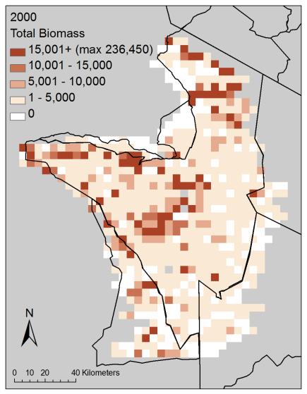
118 C) 118

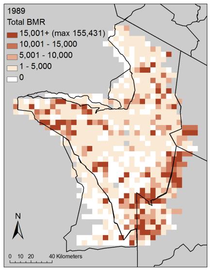
119 D) 119

120 A) B) C) D) Figure A-3. Community distributions (for sample locations at 5 km intervals) for a dry season survey in 1996: A) species richness, B) total abundance, C) total biomass (kg), D) total basal metabolic rate (W). 120

121 Appendix A-5. Habitat Characteristics Methods (with Figures). Dates for habitat data are provided in Table A-4 and A-5. Geographic Information System (GIS) analyses to prepare the habitat variables were completed in ArcGIS (ESRI 2009). Human Activity Potential impacts of human activity were represented in the analysis using the following variables: distance (m) from the park western boundary, direction (east or west) from the park western boundary, their interaction (distance x direction), and road density (km road/km 2 area). The protected area boundaries and distribution of roads are not expected to have changed over the duration of the study; however, human activities may have changed over time and are addressed in the Discussion in the main text. The distance (m) from the western park boundary was examined to investigate the influence of human activity into the interior of the park. Such influences could be because humans (e.g., poachers) or livestock wander into the park. Alternatively, wildlife could wander across the boundary and experience different conditions and the existence of the boundary could constrain movement possibilities. The western boundary of the park has distinct land use activities to its east and west (Figure A-4a). To the west, there are unprotected areas, which are highly populated, and game reserves which are intended to serve as buffer areas for the park (but do allow hunting). To the east of this boundary, there is the national park, which does not permit livestock or agriculture, and further east there are conservation areas, which allow controlled pastoralism (i.e., ranching). Poacher density is likely to decrease in relation to distance from human population, and poaching risk shows a general decrease from west to east 121

122 within the park (Metzger et al. 2007). Consequently, the interaction between distance from park western boundary and direction (west or east) was incorporated in the analysis. The distance (m) from the western park boundary was calculated for each survey grid cell by finding the distance from the center of the cell to the nearest edge on the western park boundary (Figure A-4b). Roads, which are associated with activities such as hunting and tourism, were mapped by the Tanzania Wildlife Conservation Monitoring Program and Frankfurt Zoological Society. The road types are as follows: main; all-weather; seasonal; tourist; restricted roads; and tracks and trails. Road density (km road/km 2 area) was calculated for each survey grid cell as the length of roads within a circle of radius 2.5 km (centered on the center of the survey grid cell) divided by the circle s area (Figure A-4c). Topography Topography, which can influence vegetation type (and thus forage quantity and quality) and animal movement more directly, was incorporated in the study as average elevation (m) and standard deviation of elevation (m) (to represent local heterogeneity in terrain) (Figure A-5). The average and the standard deviation of the elevation values within each 5 x 5 km survey grid cell were calculated using a digital elevation model with a 90-m 2 resolution obtained from the Shuttle Radar Topography Mission (SRTM) (Jarvis et al. 2008). Resources Resources and disturbances hypothesized to be important to large herbivores were represented using the following surrogate measures: distance to river (m), distance to permanent river (m), plant nutrients (ppm Ca, ppm Mg, percent N, ppm Na, ppm P), percent tree cover (average and standard deviation), Normalized Difference 122

123 Vegetation Index (NDVI) (average and standard deviation), rainfall (mm/month), and percent burn area. The analysis used an interaction between each of the dynamic variables (NDVI, rainfall, and burn area) and date (treated as a categorical variable). Proximity to rivers (m), which indicates water availability, was determined using a digital map of rivers prepared by the Tanzania Wildlife Conservation Monitoring Program and Frankfurt Zoological Society. The distribution of rivers is not expected to have changed over the study period. Distance to the nearest river (seasonally and permanently flowing rivers) as well as distance to the nearest permanent river were calculated using the center of each 5 x 5 km survey grid cell (Figure A-6). Plant nutrients (i.e., plant biomass nutrient concentrations), which are associated with vegetation quality, were determined for calcium, magnesium, nitrogen, phosphorus, and sodium. Methods are explained in Holdo et al. (2009); the plant nutrient data were collected by S.J. McNaughton (unpublished data) at 115 sites and interpolated by R.D. Holdo to create plant nutrient maps, which he kindly provided for this study (Figure A-7). Holdo et al. (2009) suggest the data were collected in the 1980s. Based on comparisons with subsequent independent nutrient studies, they conclude that general spatial patterns of nutrients have not changed considerably over the approximate period of Percent tree cover, which indicates the amount of woody vegetation available and thus forage for browsers (and cover from predators), was estimated using the Vegetation Continuous Fields (VCF), Collection 3 original, a product derived from Moderate Resolution Imaging Spectroradiometer (MODIS) Terra satellite data (Hansen et al. 2003). The VCF data indicates the percent of each 500 x 500 m pixel covered by 123

124 woody vegetation as an annual representation for the period Nov 2000 Nov The percent tree cover was determined for each 5 x 5 km survey grid by finding the mean of the 100 VCF pixel values within each survey grid. To represent local heterogeneity in woody cover, the standard deviation of the VCF values within each 5 x 5 km survey gird was also determined (Figure A-8). Although general patterns of tree cover have not changed appreciably during the duration of the study, tree densities have increased (Sinclair et al. 2007); such changes in tree cover may be captured by another variable in the study, NDVI. The Normalized Difference Vegetation Index (NDVI), an indicator of plant productivity, was used to represent an index of food availability for herbivores. NDVI data were obtained from two sources. For survey years prior to 2000, imagery was obtained from Advanced Very High Resolution Radiometer Global Inventory Modeling and Mapping Studies (AVHRR-GIMMS) on the NOAA satellite series 7, 9, 11, 14, 16 and 17 at an 8 x 8 km resolution (Tucker et al. 2004). The center of each 5 x 5 km survey grid cell was used to extract a corresponding NDVI value (Figure A-9). For survey years 2000 and onwards, MODIS data were obtained as 16-day composite measures at a 250 x 250 m resolution (NASA n.d.). For these years, the average of the NDVI values within each 5 x 5 km survey grid cell was calculated (Figure A-9) as well as the standard deviation of the NDVI values (to represent local heterogeneity) (Figure A- 10). For both sources, the NDVI monthly time range selected was for the dates closest to that of the survey dates (Appendix A-2). NDVI values range between -1.0 to 1.0, where increasing positive values indicate increasing amounts of green vegetation. 124

125 Rainfall, which influences vegetation type, was acquired as maps from The University of Delaware Terrestrial Precipitation: Gridded Monthly Time Series Version 2.01 (Matsuura and Willmott 2009). The rainfall data are monthly total precipitation interpolated to a 0.5 x 0.5 degree grid. A subset of the data was selected for the spatial extent of the study region. NDVI/vegetation has a 1-2 month lag in response to rainfall in savanna systems (Chamaille-Jammes et al. 2006, Shinoda 1995); thus, the average rainfall of the two months preceding the month of the survey data was determined (Appendix A-2). These values were interpolated using universal kriging with a first-order trend to a spatial resolution of approximately 1 x 1 km. The rainfall (mm/month) for each 5 x 5 km survey grid cell was selected using the corresponding value at the center of the cell (Figure A-11). Fire, which has a prominent effect on savanna vegetation structure, was represented using fire maps for produced by Dempewolf et al. (2007), who identified burned areas by applying an algorithm that uses red and near infrared reflectance values at a 250 x 250 m spatial resolution acquired by MODIS sensor. For the surveys in years 2001, 2003, and 2006 (which occurred in the wet season), maps were created for fire occurrence within the previous year (i.e., May of the prior year through April of the survey year) (Appendix A-2). As there are few fires in the wet season, the data essentially indicate fire occurrence in the prior dry season. For each 5 x 5 km survey grid cell, the proportion of 250 x 250 m cells with fire present was used as a proxy for percent burn (i.e., area of each 5 x 5 km survey grid cell burned within the prior year) (Figure A-12). 125

126 A) B) C) Figure A-4. Serengeti National Park (~15,000 km 2 ) and its neighboring conservation areas and game reserves located in Tanzania and Kenya, East Africa. Indicators of human activity at each survey location: A) protection class, B) distance (m) from western park boundary (white line is the boundary), and C) road density (km/km 2 ). CA = conservation area, GR = game reserve, NP = national park, RA = reserve area. 126

127 A) B) Figure A-5. Topography of the study area measured by A) average elevation (m) and B) standard deviation of elevation (m). CA = conservation area, GR = game reserve, NP = national park, RA = reserve area. 127

128 A) B) Figure A-6. The distance (m) from each survey location to A) the nearest river and B) to the nearest permanent river. CA = conservation area, GR = game reserve, NP = national park, RA = reserve area. 128

129 A) B) C) D) E) Figure A-7. Plant nutrient maps of: A) percent N, B) ppm Ca, C) ppm Mg, D) ppm Na, E) ppm P. CA = conservation area, GR = game reserve, NP = national park, RA = reserve area. 129

130 A) B) Figure A-8. Tree cover: A) mean percent tree cover and B standard deviation of percent tree cover within each 5 x 5 km grid cell. CA = conservation area, GR = game reserve, NP = national park, RA = reserve area. 130

131 Figure A-9. NDVI from approximately the month of each survey. A) 1988, B) 1989, C) 1991, D) 1996, E) 1996 (dry season), F) 2000, G) 2001, H) 2003, I) CA = conservation area, GR = game reserve, NP = national park, RA = reserve area. A) B) C) 131

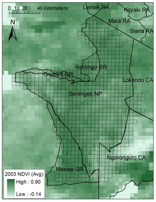
132 D) E) F) G) H) I) 132

133 A) B) C) D) Figure A-10. Standard deviation of NDVI values within each 5 x 5 km grid cell for four wet season surveys. A) 2000, B) 2001, C) 2003, D) CA = conservation area, GR = game reserve, NP = national park, RA = reserve area. 133

134 Figure A-11. Average rainfall (mm/month) for the two months preceding each survey date. A) 1988, B) 1989, C) 1991, D) 1996, E) 1996 (dry season), F) 2000, G) 2001, H) 2003, I) CA = conservation area, GR = game reserve, NP = national park, RA = reserve area. A) B) C) 134

135 D) E) F) G) H) I) 135

136 A) B) C) Figure A-12. Percent burn (area within each grid cell burned) within the prior year: A) May April 2001, B) May 2002 April 2003, C) May April CA = conservation area, GR = game reserve, NP = national park, RA = reserve area. 136