Geological Control of Floristic Composition in Amazonian Forests. Mark Higgins. University Program in Ecology Duke University.

Transcription

1 Geological Control of Floristic Composition in Amazonian Forests by Mark Higgins University Program in Ecology Duke University Date: Approved: Dr. John Terborgh, Supervisor Dr. Kalle Ruokolainen Dr. Dean Urban Dr. Daniel Richter Dissertation submitted in partial fulfillment of the requirements for the degree of Doctor of Philosophy in the University Program in Ecology in the Graduate School of Duke University 2010

2 ABSTRACT Geological Control of Floristic Composition in Amazonian Forests by Mark Higgins University Program in Ecology Duke University Date: Approved: Dr. John Terborgh, Supervisor Dr. Kalle Ruokolainen Dr. Dean Urban Dr. Daniel Richter An abstract of a dissertation submitted in partial fulfillment of the requirements for the degree of Doctor of Philosophy in the University Program in Ecology in the Graduate School of Duke University 2010

3 Copyright by Mark Higgins 2010

4 Abstract Amazonia contains the largest remaining tracts of undisturbed tropical forest on earth, and is thus critical to international nature conservation and carbon sequestration efforts. Amazonian forests are notoriously difficult to study, however, due to their species richness and inaccessibility. This has limited efforts to produce the accurate, high resolution biodiversity maps needed for conservation and development. The aims of the research described here were to identify efficient solutions to the problems of tropical forest inventory; to use these methods to identify floristic patterns and their causes in western Amazonia; and propose new means to map floristic patterns in these forests. Using tree inventories in the vicinity of Iquitos, Peru, I and a colleague systematically evaluated methods for rapid tropical forest inventory. Of these, inventory of particular taxonomic groups, or taxonomic scope inventory, was the most efficient, and was able to capture a majority of the pattern observed by traditional inventory techniques with one fifth to one twentieth the number of stems and species. Based on the success of this approach, I and colleagues specifically evaluated two plant groups, the Pteridophytes (ferns and fern allies) and the Melastomataceae (a family of shrubs and small trees), for use in rapid inventory. Floristic patterns based on inventories from iv

5 either group were significantly associated with those based on the tree flora, and inventories of Pteridophytes in particular were in most cases able to capture the majority of floristic patterns identified by tree inventories. These findings indicate that Pteridophyte and Melastomataceae inventories are useful tools for rapid tropical forest inventory. Using Pteridophyte and Melastomataceae inventories from 138 sites in northwestern Amazonia, combined with satellite data and soil sampling, I and colleagues studied the causes of vegetation patterns in western Amazonian forests. On the basis of these data, we identified a floristic discontinuity of at least 300km in northern Peru, corresponding to a 15 fold difference in soil cation concentrations and an erosion generated geological boundary. On the basis of this finding, we assembled continent scale satellite image mosaics, and used these to search for additional discontinuities in western Amazonia. These mosaics indicate a floristic and geological discontinuity of at least 1500km western Brasil, driven by similar erosional processes identified in our study area. We suggest that this represents a chemical and ecological boundary between western and central Amazonia. Using a second network of 52 pteridophyte and soil inventories in northwestern Amazonia, we further studied the role of geology in generating floristic pattern. Consistent with earlier findings, we found that two widespread geological formations in western Amazonia differ eight fold difference in soil cation concentrations and in a v

6 majority of their species. Difference in elevation, used as a surrogate for geological formation, furthermore explained up to one third of the variation in plant species composition between these formations. Significant correlations between elevation, and cation concentrations and soil texture, confirmed that differences in species composition between these formations are driven by differences in soil properties. On the basis of these findings, we were able to use SRTM elevation data to accurately model species composition throughout our study area. I argue that Amazonian forests are partitioned into large area units on the basis of geological formations and their edaphic properties. This finding has implications for both the ecology and evolution of these forests, and suggests that conservation strategies be implemented on a region by region basis. Fortunately, the methods described here provide a means for generating accurate and detailed maps of floristic patterns in these vast and remote forests. vi

7 To Leena, And those working to protect this world s natural systems. Rare is the enterprise which offers so little grounds for optimism and demands so much from our power to hope. Egbert Leigh Jr. vii

8 Contents Abstract...iv List of Tables...xii List of Figures...xiv Acknowledgements...xix Chapter 1. Introduction...1 Chapter 2. Rapid tropical forest inventory: a comparison of techniques using inventory data from western Amazonia...10 Summary...10 Introduction...11 Methods...15 Inventory data...15 Creation of abbreviated inventories...16 Evaluation of inventory abbreviations...20 Results...23 Inventory data...23 Creation of abbreviated inventories...23 Evaluation of inventory abbreviations...25 Occurrence metric analyses...25 Taxonomic resolution analyses...25 Diameter class analyses at species or genus resolution...26 Taxonomic scope analyses...28 viii

9 Discussion...30 Evaluation and comparison of inventory abbreviations...30 Presence absence occurrence metric...30 Genus resolution...31 Diameter classes at species or genus resolution...32 Taxonomic scope...33 Optimizing tropical forest inventory...35 From inventory to conservation planning...36 Acknowledgements...37 Chapter 3: Are floristic and edaphic patterns in Amazonian rain forests congruent for trees, pteridophytes and Melastomataceae?...48 Summary...48 Introduction...50 Materials and methods...53 Study sites...53 Floristic inventories...54 Soil sampling...56 Computing of distance matrices...57 Mantel tests and ordinations...59 Multiple regressions on distance matrices...60 Results...62 Floristic inventories...62 ix

10 Soils...62 Congruence between plant groups...63 Congruence between floristic, environmental and geographic patterns...65 Discussion...68 Determinants of floristic patterns...68 Are these results reliable?...71 Practical implications...73 Acknowledgements...75 Chapter 4: Long term Sub Andean Tectonics Control Floristic Composition in Amazonian Forests...87 Summary...87 Introduction...89 Results...93 Discussion...98 Materials and Methods Landsat image mosaics and image interpretation SRTM mosaics and elevation calculations Pteridophyte and Melastomataceae transect analyses Tree plot analyses Acknowledgements Chapter 5. Geological control of floristic composition in western Amazonia Introduction x

11 Methods Study area Satellite imagery acquisition and interpretation Field data collection Data analyses Results Satellite image interpretation Data analyses Discussion Overview Relationships between elevation, soils, and floristic composition Evolution of the western Amazonian biota Implications for conservation planning Chapter 6. Conclusion References Biography xi

12 List of Tables Table 1: Characteristics of presence absence and taxonomic resolution abbreviations for nine sites near Iquitos, Peru...39 Table 2: Characteristics of diameter classes at species resolution for nine sites near Iquitos, Peru. a...40 Table 3: Characteristics of diameter classes at genus resolution for nine sites near Iquitos, Peru. a...41 Table 4: Characteristics of taxonomic scope abbreviations for nine sites near Iquitos, Peru. a...42 Table 5: Characteristics of taxonomic scope combinations for nine sites near Iquitos, Peru. a...43 Table 6: Results of floristic inventories made in three regions in lowland western Amazonia. Floristic similarity between sites is calculated both with the Steinhaus index (Steinh.) (abundance data) and with the Sørensen index (Søren.) (presence absence data) Table 7 : Results of chemical and physical analyses of soils within three regions in lowland western Amazonia. Cation concentrations are given in cmol(+) kg 1, LOI (loss on ignition) and sand content in %...78 Table 8: Mantel correlations between floristic differences based on three different plant groups in three western Amazonian regions. Partial Mantel tests, where the effect of geographical distances has been removed before computing the correlation between the two floristic distance matrices, are shown in parenthesis. Sørensen index uses species presence absence data, Steinhaus index abundance data. Statistical significances were obtained by a Monte Carlo permutation test using 999 permutations: *** P < 0.001, ** P < 0.01; * P < The probability of obtaining a significant correlation coefficient by chance at the P < 0.05 level is 1 out of 20 tests, i.e. clearly lower than found here Table 9: Mantel correlations between floristic differences based on different plant groups in three western Amazonian regions. The Sørensen index (presence absence data) was used in all cases. Statistical significances were obtained by a Monte Carlo permutation test using 999 permutations: *** P < 0.001, ** P < 0.01; * P < The probability of xii

13 obtaining a significant correlation coefficient by chance at the P < 0.05 level is 1 out of 20 tests, i.e. clearly lower than found here Table 10: Mantel correlations between floristic differences and either edaphic or geographical distances in three regions of lowland western Amazonia. Three different plant groups were analysed separately using either the Steinhaus index (St; abundance data) or the Sørensen index (Sø; presence absence data). LOI = loss on ignition. Edaphic differences were based on the Euclidean distance. The highest correlation coefficient of an edaphic variable for each region is shown in bold. Statistical significance of each correlation coefficient was assessed with a Monte Carlo permutation test using 999 permutations. *** P < 0.001, ** P < 0.01, * P < 0.05, P < 0.1 (the last probability level is indicated to facilitate comparison with Fig. 3). The probability of obtaining a significant correlation coefficient by chance at the P < 0.05 level is 1 out of 20 tests, i.e. clearly lower than found here Table 11: Indicator species analysis results for pteridophyte species Table 12: Indicator species analysis results for Melastomatacae species Table 13: Indicator species analysis results for tree species Table 14: Results of indicator species analysis for Pteridophyte species Table 15: Soil properties for 52 sites in northwestern Amazonia Table 16: Correlations between floristic composition and environmental variables Table 17: Pairwise correlations between environmental variables Table 18: Comparison of observed and predicted floristic classes xiii

14 List of Figures Figure 1: Location of the nine study sites near Iquitos, Peru...44 Figure 2: Comparison of diameter classes, diameter classes at genus resolution, and taxonomic scope to random sampling. Comparison of each group to random sampling in terms of (a to c) mean number of stems per site or (d to f) total number of taxa. The two lines represent the 95% confidence interval for random sampling. Crosses in (c) and (f) are 13 taxa combination groups composed of pairs of familes or genera with individually high r values. Regression models for the three groups for (g) number of stems per site versus correlation or (h) total number of taxa versus correlation. (i) height of stems versus r value for the three groups. Filled squares in (g) to (i) are taxonomic scope abbreviations, crosses are diameter classes at genus resolution, and open squares are diameter classes; taxa combinations not included...46 Figure 3: Mean performance of inventory methods for nine sites near Iquitos, Peru. Positions represent the mean number of stems and taxa for each type of inventory for all abbreviations with r 0.71 (abundance data only) Figure 4: Map of the study area. Circled areas indicate the approximate locations of the three study regions: Yasuní (in Ecuador), Loreto (northern Peru) and Madre de Dios (southern Peru)...82 Figure 5: Geographical locations of the study sites within each of three study regions (a, Madre de Dios; b, Loreto; c, Yasuní; latitude and longitude indicated in degrees), and floristic ordinations (Principal Coordinates analysis based on the Sørensen index) as obtained for each of three plant groups separately (d f, trees; g i, pteridophytes; j l, Melastomataceae). The diameter of the circles is proportional to the mean concentration of exchangeable bases (Ca + K + Mg + Na) in the corresponding site relative to that in the other sites in the same region. The cumulative eigenvalues of the first two axes in the ordinations were 41 76%. For the location of the three regions, see Figure Figure 6: Results of variation partitioning of floristic differences (as based on multiple regression on distance matrices) in three regions of lowland western Amazonia. Trees (tr.), Pteridophytes (Pteridoph.) and Melastomataceae (Melast.) were analysed separately using either the Sørensen index (presence absence data, left) or the Steinhaus index (abundance data, right). Edaphic differences were based on the Euclidean distance. The soil variables retained in a backward elimination procedure, and hence included in the final analysis, are shown in each case (LOI = loss on ignition). xiv

15 Proportions of variation explained: a = uniquely explained by the edaphic differences; b = jointly explained by the edaphic and geographical distances; c = uniquely explained by the geographical distances; d = unexplained. Since fraction b is obtained by subtraction, it may be either positive or negative Figure 7: Relationship between remotely sensed discontinuity, plant species composition, and soil cation concentrations. Yellow line indicates the discontinuity identified in Landsat (A) and SRTM (B) data, between the Miocene Pebas Formation (north of discontinuity) and Late Miocene Nauta Formation (south of discontinuity). From left to right, insets show detail of Pastaza Fan; detail of northwest of study area; location of study area; and detail of the upper Pucacuro river. (A), Results of floristic clustering analyses superimposed upon Landsat mosaic for study area. Circles indicate transects with both pteridophyte and Melastomataceae inventories, and triangles indicate transects with only pteridophyte inventories. The color of a transect indicates its classification by clustering analysis, which was used to generate two groups (main figure) or four groups (center left inset). For the latter, a group of three inventories restricted to the southeast of the study area is not displayed. (B), Soil cation concentrations superimposed upon a SRTM digital elevation model for the study area. Diameter of circles is proportional to the log transformed sum of the concentrations of four cations (Ca, Mg, Na, and K). Light tones in the digital elevation model indicate higher elevation, and dark tones lower elevation. Maximum elevation in the study area is 433m, and minimum is 98m. Dark red tones in Landsat imagery (A) along rivers and in the south of the study area indicate inundated forest or swamp; and white patches in northwest and north of study area are clouds Figure 8: Boundary between Miocene and Late Miocene Pleistocene sediments, relative to continent scale SRTM and Landsat mosaics. Boundary is indicated by yellow line and divides dissected Miocene Pebas sediments in the west from planar Late Miocene Pleistocene sediments in the east. (A), SRTM digital elevation model for Amazonia. Light tones indicate higher elevation and dark tones lower elevation. Green box indicates the extent of figure 7, blue box indicates the extent of figures 2B and C, and inset indicates location relative to South America. (B), Landsat mosaic for the area indicated by blue box in A, with major rivers labeled. (C) SRTM digital elevation model for the same area for same area as B. Maximum and minimum elevations in A are 6157m and 0m, and in C are 779m and approximately 40m Figure 9: Landsat data used for Figure 7. Black outlines represent image areas, and red outline indicates mosaic area. Top value for each image indicates path and row combination for the image, and bottom value indicates day, month, and year xv

16 Figure 10: Landsat data used for Figure 8. Black outlines represent image areas, and red outline indicates mosaic area. Top value for each image indicates path and row combination for the image, and bottom value indicates day, month, and year Figure 11: Landsat mosaic and interpretation for study area. Mosaic consists of four overlapping images (see Figure 13) comprised of bands 4, 5, and 7, set to display in red, green, and blue, respectively. Image interpretation is overlaid in yellow. Red tones along rivers indicate swamp forests and white area in center of image represents clouds Figure 12: SRTM data for study area. Light tones indicate high elevations and dark tones low elevations. Image interpretation is overlaid in blue. Elevation ranges from 120 to 320 meters Figure 13: Landsat images used to construct Landsat mosaic. Black lines indicate image outlines and red box indicates extent of mosaic. Upper value for each image indicates path and row of image, and bottom value indicates the image date Figure 14: Location of plant inventories. Green points represent 52 fern inventories esatblished during Yellow lines indicate boundaries between poor soil islands and rich soil matrix. Landsat mosaic consists of bands 4, 5, and 7, set to red, green, and blue Figure 15: Results of clustering analysis for fern inventories. Red and blue points indicate fern inventories, classified into twogroups. Green lines indicate boundaries between poor soil islands and rich soil matrix. Map location and scale as in Figure Figure 16: Cation availability at inventory sites. Circles indicate inventory sites, and diameter of circles indicates cation availability, measured as the log transformed sum of Mg, Ca, Na, and K concentrations. Green lines indicate boundaries between poor soil islands and rich soil matrix. Map location and scale as in Figure Figure 17: NMDS ordination of floristic data and correlations with soil properties. Horizontal axis is axis I and vertical axis is axis II. Blue triangles indicate transects, and red vectors indicate strength of correlation of environmental variables with ordination axes. Vectors for Log Na and P are obscured behind Log K and ph, respectively Figure 18: Relationship between clustering groups, ordination axes, and two environmental variables. Horizontal axis is NMDS axis I and vertical axis is NMDS axis II. Color of points indicates clustering group (red for Nauta group, and blue for Pebas xvi

17 group) and diameter indicates (A, top) cation concentration (log transformed sum of Mg, Ca, K, and Na), or (B, bottom) percent clay Figure 19: Regression of cation concentrations on NMDS axis I. X axis represents the logtransformed sum of cation concentrations (Mg, Ca, K, and Na), and Y axis represents positions on NMDS axis I. Color of points indicates clustering group (red for Nauta group, and blue for Pebas group) and diameter indicates elevation. Y axis crosses X axis at cation threshold identified by CART analysis ( ) Figure 20: Regression of clay content on NMDS axis I. X axis represents percent clay, and Y axis represents positions on NMDS axis I. Color of points indicates clustering group (red for Nauta group, and blue for Pebas group) and diameter indicates elevation. Y axis crosses X axis at percent clay threshold identified by CART analysis (59.4%) Figure 21: Regression of elevation on NMDS axis I. X axis represents elevation, and Y axis represents positions on NMDS axis I. Color of points indicates clustering group (red for Nauta group, and blue for Pebas group) and diameter indicates cation concentration (log transformed sum of Mg, Ca, K, and Na). Y axis crosses X axis at elevation threshold identified by CART analysis ( m) Figure 22: Regression of elevation on cation concentration. X axis represents elevation, and Y axis represents cation concentration (log transformed sum of Mg, Ca, K, and Na). Color of points indicates clustering group (red for Nauta group, and blue for Pebas group). Y axis crosses X axis at elevation threshold identified by CART analysis ( m), and X axis crosses Y axis at cation threshold ( ) Figure 23: Regression of elevation on clay content. X axis represents elevation, and Y axis represents percent clay. Color of points indicates clustering group (red for Nauta group, and blue for Pebas group). Y axis crosses X axis at elevation threshold identified by CART analysis ( m), and X axis crosses Y axis at percent clay threshold (59.4%) Figure 24: Classified SRTM for study area. Values of 1 (white) indicate areas classified by elevation as Nauta Formation forest (elevation greater than m), and values of 0 (black) indicated areas classified as Pebas Formation forest (elevation less than m). Image interpretation is overlaid in blue Figure 25: Relationship between floristic composition and regional geological patterns. Labeled patches represent geological formations and yellow lines indicate boundaries identified in this study. Geological formations are as follows: NQ ns = Neogene to xvii

18 Quaternary, Nauta superior; NQ ni = Neogene to Quaternary, Nauta inferior; N p = Neogene, Pebas; Qp al = Pleistocene alluvial deposition; Qh al = Holocene alluvial deposition.; N i = Ipururo formation (INGEMMET 2000) xviii

19 Acknowledgements The road from molecular biology to tropical ecology is neither well trodden nor short, and I am indebted to those who aided and accompanied me along the way. John Terborgh, my advisor, provided a home at Duke University, and a beacon for many years of the possibilities of tropical ecology and tropical forest conservation. I am particularly grateful to Kalle Ruokolainen for over a decade of support and friendship. Academia can be a prickly and lonely place, and Kalle s encouragement, collaboration, and assistance have been invaluable. Hanna Tuomisto patiently instructed me in every detail of the field methods that are the bread and butter of this work; taught me the western Amazonian pteridophytes; and identified countless near identical specimens long after my eyes had crossed. Dean Urban, Pat Halpin, and Dan Richter, my committee members, provided valuable time and feedback. The Amazon Research Team at the University of Turku, Finland, provided a home, companionship, and inspiration during my time in Finland. My research was generously supported by a variety of institutions, including the National Science Foundation (USA), whose Graduate Research Fellowship program provided the three years of no strings attached funding needed to pursue a project xix

20 many said was impossible; the American Scandinavian Foundation and the Center for International Mobility (Finland), which together funded two year of collaboration with colleagues at the Unversity of Turku, Finland; and the Duke Graduate School, Latin American Studies Program, and Sigma Xi Society, who provided funding for travel and equipment during two years of fieldwork. I would also like to thank Joe Kolowski and Sulema Castro at the Smithsonian Institution for making the research described in chapter five both possible and a great time to boot. I would also like to thank Alfonso Alonso for making this fieldwork possible, and for inviting me to join it. I am indebted to those who assisted in the field, and particularly Eneas Perez and Nydia Elespuru, whose fieldwork provided a major contribution to chapter five; and Fernando Ruiz, Apu of the Nuevo Remanente community, for unwavering assistance on over 80 field inventories along the Tigre and Pastaza rivers, and the forest between. Many others assisted with individual parts of this project, and they are acknowledged at the end of the chapters to which they contributed. And above all, I thank my fiancée Leena Kemppainen, and my mother, father, and brother, for the love, support, and no small amount of patience that made this work possible. xx

21 Chapter 1. Introduction Amazonia contains the largest remaining tracts of undisturbed tropical forest on earth. These forests harbor the most diverse plant and animal communities known to science (Gentry 1988, Valencia et al. 1994), and store and process globally significant amounts of carbon (Malhi et al. 2008, Phillips et al. 1009). Amazonian forests are thus of the utmost importance to the earth s carbon budget and to the goal of conserving biodiversity. However, the physical and technical challenges of research in the remote expanses of this continent sized area have stifled efforts to produce the biodiversity maps needed for conservation and development planning (Margules and Pressey 2000, Noss et al. 1999). As a result, knowledge of the biota of much of Amazonia remains in what John Terborgh has termed the stone age (Terborgh 1992). UNESCO maps for Amazonia, an area roughly two thirds the size of the continental United States, recognize a scant half dozen vegetation types (Terborgh and Andresen 1998, commenting on UNESCO 1980), in comparison to the estimated 4100 types recognized for the United States (Grossman et al. 1998). Large area maps, furthermore, are generally based on surrogate environmental variables or expert opinion rather than field data (Dinerstein et al. 1995). Accurate vegetation maps, supported by a clear understanding of the causes of floristic patterns, are thus crucial for both the study and conservation of Amazonian forests. 1

22 Soil properties are known to control plant species distributions in tropical forests at sites ranging from central America, to southeast Asia, to the expanses of Amazonia (Duivenvoorden 1995, Duque et al. 2009, Honorio et al. 2009, John et al. 2007, Palmiotto et al. 2004, Phillips et al 2003, Salovaara 2004, Tuomisto et al. 2003c). Within Amazonia, large area patterns in soil properties are believed to have produced long distance and possibly abrupt patterns in floristic composition, driven by the Andean orogeny (Ter Steege et al. 2000, Ter Steege et al. 2006). This raises the possibility that underlying geological processes may control floristic composition in Amazonia (Ter Steege et al. 2006, Tuomisto et al. 1995, Pitman et al. 2008). This would provide a general model for floristic patterns in these forests, and open new avenues for their mapping and study. The objective of my research was to study the relationship between geological and floristic patterns in a sector of northwestern Amazonia; and to use this information to map these patterns. Geological study in western Amazonia has revealed a complex history of depositional and erosional events, dating to the Miocene and driven by the Andean orogeny. These processes have generated a widespread mosaic of geological formations of varying size, age, and properties, much of which is documented in national geological maps (IMGEMMET 2000, Schobbenhaus et al. 2004). The implications of these patterns for floristic composition are poorly known, however, and this relationship has been difficult to test due to a lack of large area but detailed floristic, edaphic, and geological datasets. 2

23 One challenge to studies of plant compositional patterns in Amazonian forests is a lack of plant inventory data. Floristic inventory in the Neotropics is notoriously difficult due to extremely large numbers of species (Duivenvoorden 1994; Valencia et al. 1994; Ter Steege et al. 2000; Pitman et al. 2001), the poor state of their taxonomy (Prance 1994), and the difficulties of field identification. For at least 50 years, the dominant solution to these problems has been to restrict sampling to the tallest trees in the forest (Campbell 1989; Ter Steege et al and references therein). This technique, however, remains time consuming, and requires the identification of large numbers of individual trees, almost all of which are tall and thus difficult to voucher and identify (e.g., Pitman et al. 2001; Condit et al. 2002). More efficient solutions to the challenges of forest inventory would thus be a boon to the mapping and study of these forests. A second challenge to studying patterns in these forests is their inaccessibility. Road networks are absent from much of Amazonia, and western Amazonia is particularly inaccessible. Though inaccessibility has so far inhibited large scale colonization, it has also hindered biological exploration. Inventories have typically been limited to sites close to population centers and along rivers, and large expanses of forest in interfluvial zones thus remain unsampled. Remotely sensed (e.g. satellite) data offers a potential solution to these problems. Patterns in Landsat imagery can be used to identify changes in plant species composition, and geomorphological features in SRTM (Shuttle Radar Topography Mission) elevation data can be used to identify geological 3

24 formations (Tuomisto et al. 2003a, Thessler et al. 2005, Rossetti and Valeriano 2007). Such data offer the possibility of extrapolating patterns of geology and vegetation from inventoried areas into blank regions of the map. These satellite datasets are furthermore highly accurate and publicly available, making them very well suited to the needs of conservation planners. To meet these challenges, I evaluated a variety of methods for accelerating tropical forest inventories, and specifically tested two plant groups for their use in rapid forest inventory in Amazonia. I then combined these plant inventories with satellite imagery and soil sampling to study the relationship between vegetation and geology over a much larger expanses of Amazonian forest. I conclude that Amazonian forests are partitioned into large area units on the basis of geological formations and their soil properties, and demonstrate the use of satellite imagery to map these patterns. This research provides a general model for the creation of vegetation patterns in Amazonian forests, and new tools for mapping these patterns. This work is described in four chapters, written as research articles. Following are brief summaries: Chapter 2: Rapid tropical forest inventory: a comparison of techniques using inventory data from western Amazonia Co author: Kalle Ruokolainen (Univ. of Turku, Finland) 4

25 Published: Conservation Biology, 2004, 18: Using tree inventories in the vicinity of Iquitos, Peru, we systematically evaluated methods for rapid tropical forest inventory, including the use of presenceabsence data; identification of specimens only to genus or family; the inventory of only particular diameter classes; and the inventory of only particular taxonomic groups (either families or genera). Of these methods, inventory of particular taxonomic groups, or taxonomic scope inventory, was the most efficient, and was able to capture a majority of the information yielded by traditional inventory techniques with one fifth to one twentieth the number of stems and species. Chapter 3: Are floristic and edaphic patterns in Amazonian rain forests congruent for trees, pteridophytes and Melastomataceae? Co authors: Kalle Ruokolainen (Univ. of Turku, Finland), Hanna Tuomisto (Univ. of Turku, Finland), Manuel Macia (Real Jardın Botanico de Madrid, Spain), and Marku Yli Halla (MTT Agrifood Research, Finland) Published: Journal of Tropical Ecology, 2007, 23:13 25 Based on the success of taxa based inventory, we specifically evaluated two plant groups, the Pteridophytes (ferns and fern allies) and the Melastomataceae (a family of 5

26 shrubs and small trees), for use in rapid inventory, using plant inventories in Iquitos (Peru), Madre de Dios (Peru), and the Yasuní National Park (Ecuador). The patterns of similarity between sites based on inventories of these two plant groups were significantly correlated with patterns based on tree species composition in all but one case (Melastomataceae at Yasuni). Inventories of Pteridophytes, in particular, were able to capture the majority of floristic patterns identified by tree inventories in two of three regions. These findings indicate that Pteridophyte and Melastomataceae inventories are useful tools for rapid tropical forest inventory. Chapter 4: Long term Sub Andean Tectonics Control Floristic Composition in Amazonian Forests Co authors: Kalle Ruokolainen (Univ. of Turku, Finland), Hanna Tuomisto (Univ. of Turku, Finland), Nelly Llerena (Univ. of Turku, Finland), Glenda Cardenas (Univ. Particular de Iquitos, Peru), Oliver Phillips (University of Leeds, UK), Rodolpho Vasquez (Missouri Botanical Gardens, USA), and Matti Räsänen (Univ. of Turku, Finland) Using Pteridophyte and Melastomataceae inventories from 138 sites in northwestern Amazonia, combined with satellite data and soil sampling, we studied the correlates of vegetational heterogeneity in western Amazonian forests. Geological 6

27 studies of western Amazonia indicate a complex history of deposition and erosion, dating to the Miocene and culminating in two dominant patterns: a long frontier in western Brasil between the cation rich Pebas Formation and cation poor Ica Formation (found in western and central Amazonia respectively); and a matrix of cation rich Pebas Formation in western Amazonia containing elevated islands of more recent, cation poor sediments. Our objective was to determine the importance of these geological patterns for floristic composition. On the basis of these data, we identified a floristic discontinuity extending over at least 300km in northern Peru, corresponding to a 15 fold difference in soil cation concentrations and an erosion generated geological boundary. This boundary corresponded to a division between the widespread, cation rich Pebas Formation, and a higher elevation island of cation poor sediments (the Nauta Formation). Furthermore, this boundary was clearly visible as matched patterns in SRTM (Shuttle Radar Topography Mission) elevation data, and Landsat imagery. On the basis of this finding, we assembled continent scale SRTM and Landsat mosaics and used these to examine the long boundary between the Ica and Pebas Formations. These mosaics indicate a floristic and geological discontinuity of at least 1500km, driven by similar erosional processes identified in our study area, and we suggest that this represents a chemical and ecological boundary between western and central Amazonia. 7

28 Chapter 5: Geological control of floristic composition in Amazonian forests Co authors: Eneas Perez, Nydia Elespuru, Alfonso Alonso (Smithsonian Institution, USA) Using a second network of 52 pteridophyte and soil inventories in northwestern Amazonia, we studied further the contrast between mesa like islands of cation poor Nauta Formation and the underlying Pebas Formation matrix. Consistent with our previous findings, these geological formations differ 8 fold in soil cation concentrations, and a majority of species are significantly associated with one of the two formations. Furthermore, differences in elevation, used as a surrogate for geological formation, explained up to one third of the variation in plant species composition. Significant correlations between elevation, and cation concentrations and soil texture, confirmed that differences in species composition between these formations are driven by differences in soil properties. On the basis of these findings, we were able to use SRTM elevation data to accurately model species composition throughout our study area. The work reported here was done in collaboration with colleagues at a variety of institutions, and these collaborators are listed as co authors on the above chapters. These 8

29 chapters are thus written in the first person plural. In addition, chapters two and three, have been published in the journals noted above. 9

30 Chapter 2. Rapid tropical forest inventory: a comparison of techniques using inventory data from western Amazonia Co author: Kalle Ruokolainen, Department of Biology, Univerity of Turku, 20100, Finland. Summary Floristic inventory is critical for conservation planning in tropical forests. Tropical forest inventory is hampered by large numbers of species, however, and is usually abbreviated by sampling only the tallest trees in the forest, an approach that remains time consuming. In a systematic effort to identify better means of abbreviating inventory in western Amazonia, we defined four classes of inventory abbreviation and evaluated them for use in inventory: occurrence metric, the occurrence metric measured for individual taxa (e.g., presence absence); taxonomic resolution, the taxonomic level to which stems are identified; diameter class, the diameter classes to be included in inventory; and taxonomic scope, the taxon or taxa to be included in inventory. Using these four classes and all their possible combinations, we defined > 300 inventory abbreviations and evaluated them using nine inventories near Iquitos, Peru. We 10

31 evaluated these abbreviations by four criteria: correlation between the floristic patterns of the full and abbreviated inventories; mean number of stems per site; total number of taxa; and height of inventoried stems. Presence absence inventories were generally interchangeable with abundance inventories, regardless of the use of other abbreviations. Genus resolution inventory captured 80 % of the floristic pattern of the full inventory with an 80 % reduction in number of taxa sampled, but did not reduce the number of stems sampled. Diameter class based inventories, using either species or genus identifications, revealed a majority of the floristic pattern of the full inventories with a fraction of the stems and taxa, but were indistinguishable in efficiency from random sampling. Taxonomic scope abbreviations were more efficient than any other type of inventory, including random sampling, and required one fifth the number of stems and taxa of diameter class based methods and one twentieth the number of a full inventory. We believe that taxa based inventory may provide the optimal instrument for biological survey and conservation planning in western Amazonia. Introduction Floristic inventory is critical for conservation planning and management in terrestrial systems. At regional scales, inventory enables the production of vegetation maps (Sayre et al. 2000) and thus the design and management of representative reserve 11

32 networks (Noss et al. 1999; Margules & Pressey 2000). At the continental scale, inventory and vegetation maps permit the definition of large area administrative and planning units, ecoregions, within which conservation planning and management occur (Olson et al. 2001; Wikramanayake et al. 2002). Floristic inventory in the Neotropics is notoriously difficult due to the extremely large numbers of species (Duivenvoorden 1994; Valencia et al. 1994; Ter Steege et al. 2000; Pitman et al. 2001), the poor state of their taxonomy (Prance 1994), and the difficulties of field identification. For at least 50 years, the dominant solution to these problems has been to restrict sampling to trees 10 cm diameter at breast height (dbh; Campbell 1989; Ter Steege et al and references therein), the tallest trees in the forest. This method is intended to reduce the number of stems and taxa in inventory while capturing a representative sampling of the local flora. The popularity of this method is also due to historical logging interests, the conspicuous nature of canopy trees, and their structural dominance in tropical forests (Webb et al. 1967; Campbell 1989). Despite decades of use in tropical forests across the world, the ability of tall trees to represent regional or continental floristic patterns has never been evaluated. More importantly, this technique is time consuming, requiring large numbers of individuals and massive numbers of taxa, almost all of which are tall and thus difficult to collect and identify (e.g., Pitman et al. 2001; Condit et al. 2002; see below). This has limited 12

33 inventory in the Neotropics, and particularly western Amazonia, forcing researchers to extrapolate large area patterns from a small number of sites (Pitman et al. 1999; Pitman et al. 2001; Condit et al. 2002). Not surprisingly, estimates of the degree of compositional heterogeneity in western Amazonia currently vary by two orders of magnitude from homogeneity over thousands of kilometers (Pitman et al. 2001) to pervasive heterogeneity over distances as small as km (Tuomisto et al. 1995, 2003a). This uncertainty has profound implications for the protection of these forests. Compositional homogeneity throughout western Amazonia could be a boon for conservation, as effective conservation may require a relatively small number of protected areas, any of which might be planned and managed by a single nation. Widespread heterogeneity, however, would require a more substantial, transnational network of protected areas and thus cooperative planning and management. The sole means of reconciling these positions and different prescriptions for conservation planning is an extensive, systematic program of inventory in western Amazonia (Olson et al. 2002; see below). This, in turn, requires more efficient solutions to the challenges of tropical forest inventory. The simplest way to accelerate inventory is to reduce the number of individuals and taxa in inventory and the amount of information collected for these stems a process we refer to as inventory abbreviation. Many means of abbreviating inventory are available other than the sampling of tall trees, and we have identified four classes of 13

34 inventory abbreviations: the sampling only of particular diameter classes; the sampling only of a particular taxon or taxa; the identification of stems only to genus or family; and the use of the presence absence occurrence metric. Although each of these abbreviations has been used in tropical forest inventory, only three studies have evaluated a subset of these for this purpose (Webb et al. 1967; Ruokolainen et al. 1997; Kessler & Bach 1999). Furthermore, abbreviations from each class may be used both alone and in combination with those from every other class. We evaluated these four classes of inventory abbreviations, alone and in all possible combinations, for a total of 15 types of inventory abbreviations and over 300 individual inventory abbreviations. This represents the first systematic evaluation of inventory methodologies, including the dominant 10 cm dbh (diameter at breast height) diameter class, for any tropical forest. In addition, these evaluations were directly comparable, allowing us to identify the most efficient means of inventorying the forests in our study area. Though our findings are limited to western Amazonia, the methods we describe can be applied to any tropical forest. We thus believe these findings may encourage a new generation of tropical forest inventory techniques and enable tropical conservation planning at previously impossible scales. 14

35 Methods Inventory data We used tree inventories at nine lowland sites (approximately m above sea level) near Iquitos, Peru, to evaluate inventory abbreviations (Fig. 1; dataset described in Ruokolainen et al. [1997] and Ruokolainen & Tuomisto [1998]). The climate of this area is humid (annual precipitation 3000m) and hot (average 26º), and the sites were located in undisturbed lowland terra firme rainforest. As such these sites are typical of the forests of western Amazonia and by some accounts lie within a single floristic unit that extends for 1000s of km (Prance 1990). The sites were selected to represent regional variations in geology or satellite image reflectance, and were distributed along a soil nutrient gradient ranging from poor loamy soils to richer clayey soils. Our inventories consisted of four 20 m by 20 m plots (0.16 ha total area) distributed along 1.3 km transects. These plots were placed such that only closed canopy forest was sampled and such that two of the four plots were placed on hilltops and two in valley bottoms. This design was intended to avoid recent tree fall gaps and ensure a representative sampling of the local flora. At each plot Ruokolainen and colleagues 15

36 identified all woody, free standing stems 2.5 cm dbh to species or morphospecies, estimated their heights, and measured their dbh. Our full inventories thus consist of lists of species with stems 2.5 cm dbh and the abundance of these species. Species and morphospecies were treated equivalently during all analyses. Creation of abbreviated inventories We created abbreviated inventories for our nine sites using four classes of inventory abbreviations: (1) diameter class, the diameter classes to be included in inventory (e.g., 10 cm dbh, 3 to 4 cm dbh); (2) taxonomic scope, the taxon or taxa to be included in inventory (e.g., the Melastomataceae, Eschweilera plus Pithecellobium); (3) taxonomic resolution, the taxonomic level to which stems were identified (family, genus, species); and (4) occurrence metric, the occurrence metric measured for individual taxa (e.g., presence absence, abundance classes, abundance). Within each of these classes we selected individual inventory abbreviations and used these to create our abbreviated inventories. We selected two occurrence metrics, presence absence and abundance (number of stems per site). We also selected three degrees of taxonomic resolution: species, genus, and family. Unidentified genera (353 individuals, 8.9% of all stems) or families (18 individuals, < 1% of all stems) were excluded from abbreviated inventories at genus or family resolution, respectively. 16

37 We selected three commonly used tall diameter classes ( 10, 15, and 20 cm dbh) and either 14 or 27 short diameter classes, depending on their taxonomic resolution (see below). Short diameter classes were those for which 70% of the stems were 7 m in height, and tall diameter classes were those for which < 70% of stems were 7 m in height. This rule was chosen because identifiable material is easily collected from trees 7 m in height (i.e., these trees do not require tree climbing or long telescoping pruners) and because 70% represents a majority of stems. This rule also separated understory taxa from canopy groups and is preferable to mean or median height because these measures are not sensitive to differences in numbers of tall stems when large numbers of short stems are also present (e.g., when comparing the effective height of taxa, all of which have many individuals in small diameter classes). We chose our short diameter classes by a systematic search for short classes. During this process, we created nested sets of short diameter classes at 0.5 cm intervals by adding diameter classes of increasing length (at 0.5 cm increments) to each set until < 70% of stems in the new diameter class were 7 m in height or until we generated a diameter class that correlated with the full inventories with an r 0.8 (Pearson correlation between distance matrices of full and abbreviated inventories; see below), whichever came first. This process was conducted with both species and genusresolution data, and resulted in 14 species resolution diameter classes and 27 genusresolution diameter classes. 17

38 To ensure comparability of species and genus resolution diameter classes in later analyses (comparison of individual categories to random samples and regression analyses), all diameter classes represented at genus resolution but not at speciesresolution were also generated at species resolution (an additional 13 species resolution diameter classes; characteristics not reported in detail). Lastly, because this process did not generate a set of diameter classes with a sufficiently wide range of stem numbers, taxa numbers, or stem heights for later analyses, we generated an additional 16 diameter classes using both species and genus resolution data (characteristics not reported in detail; chosen without knowledge of r values): 5.5 to < 6 cm, 6 to < 6.25 cm, 6.25 to < 6.5 cm, 6.5 to < 7 cm, 7 to < 8 cm, 8 to < 8.5 cm, 8.5 to < 9 cm, 9 to < 9.5 cm, 9.5 to < 13 cm, 13 cm, 5 to 6 cm, 6 to 7 cm, 7 to 8 cm, 8 to 9 cm, 9 to 10 cm, and 2.5 to 10 cm. In total, our analyses employed 46 diameter classes identified to both genus and species. We selected the 10 most species rich and abundant families and genera for a total of 14 families and 16 genera. We did not evaluate individual species because it is unlikely that one species could represent the floristic pattern of the full inventories. Of the chosen families and genera, one family (the Chrysobalanaceae) and four genera (Rinorea, Mabea, Licania, and Micropholis) lacked stems at one of the nine sites and were excluded from the analyses. The 13 families selected for the taxonomic scope analyses were thus, in order of abundance, the Leguminosae, Myristicaceae, Euphorbiaceae, Burseraceae, Lecythidaceae, Sapotaceae, Meliaceae, Violaceae, 18

39 Annonaceae, Moraceae, Rubiaceae, Lauraceae, and Myrtaceae; and the 12 genera were, in order of abundance, Eschweilera (Lecythidaceae), Protium (Burseraceae), Guarea (Meliaceae), Virola (Myristicaceae), Inga (Leguminosae), Iryanthera (Myristicaceae), Siparuna (Monimiaceae), Pithecellobium (Leguminosae), Sloanea (Eleocarpaceae), Miconia (Melastomataceae), Pouteria (Sapotaceae), and Trichilia (Meliaceae). We also selected the most abundant and species rich, short stature families and genera. Short stature families and genera were those for which 70% of stems were 7 m in height. These families or genera were, in order of abundance, the Meliaceae, Violaceae, Rubiaceae, Myrtaceae, Melastomataceae, Flacourtiaceae, Nyctaginaceae, Guarea (Meliaceae), Trichilia (Meliaceae), and Neea (Nyctagniaceae). The only additional taxa selected by this criterion were thus the Nyctaginaceae, Flacourtiaceae, Melastomataceae, and Neea. We selected a number of family family and genus genus combinations. Due to the large number of possible combinations, we did not test all pair wise combinations of taxa. Instead, families and genera were selected by their correlation with the full inventories, their height, their stem and taxa numbers, the ease with which they are spotted in the field, the ease of their morphospecies identifications, and their taxonomic status (see below for a description of these criteria). These taxa combinations thus do not represent an unbiased sampling of all the possible combinations of taxa but instead 19

40 illustrate the potential of taxonomic scope abbreviations. In total, our taxonomic scope analyses included 16 families, 13 genera, and 13 combinations of families and genera. After selecting our abbreviations we created abbreviated inventories for the nine sites. Abbreviations from each of the four classes were used alone and in combination with all other abbreviations under the constraint that abbreviations from the same class were not combined (i.e., we did not use more than one diameter class and one taxonomic scope per abbreviation). The only exceptions to this rule were the thirteen taxa combinations noted above. We created our abbreviated inventories by selecting stems of the appropriate taxa or diameter class from the full inventories; identifying these to family, genus, or species; and recording their abundance or presence absence. Evaluation of inventory abbreviations We used four criteria to evaluate inventory abbreviations: (1) correlation between the floristic patterns of the abbreviated inventories and the full flora (Pearson s r); (2) mean number of stems per site; (3) total number of taxa across the nine sites; and (4) height of inventoried stems measured as the percentage of stems 7 m tall. The first criterion ensures that abbreviations will yield inventories that represent the floristic pattern present in the full flora. The second and third criteria reduce the number of vouchers to be collected, the number of potentially time consuming identifications that 20

41 must be made, and the number of specimens submitted to experts. The fourth criterion minimizes stem height and thus the difficulty of collecting identifiable material. We used the Pearson correlation coefficient (r) to measure the ability of abbreviated inventories to represent the floristic patterns of the full dataset. Pearson s r was calculated as the correlation between the distance matrix for the full inventories and that for the abbreviated inventories. A distance matrix is a square, symmetric matrix in which rows and columns are sites (also called a site x site matrix) and cells are the floristic distance between pairs of sites (e.g., percent shared species for presence absence data or percent individuals of shared species for abundance data). A single distance matrix thus represents the floristic pattern amongst sites for a single set of inventories. By comparing the distance matrix of each abbreviated inventory with that of the full inventory, we were able to measure the correlation between the floristic patterns revealed by the full and abbreviated inventories (Kent & Coker 1992: 91 96; Sokal & Rohlf 1995: ; Tuomisto et al. 1995; Ruokolainen et al. 1997; Tuomisto et al. 2003a). We calculated floristic distance between sites with the Jaccard coefficient for presence absence data and the Bray Curtis coefficient for abundance data (Legendre & Legendre 1998). Distances for the full inventories were calculated with the Bray Curtis index, and stems in the full inventories were identified to species. All correlation coefficients were calculated with PC ORD (McCune & Mefford 1999). The square of Pearson s r is the percentage of floristic variation in the full inventories captured by the 21

42 abbreviated inventory. An r value 0.71 thus indicates that the abbreviated inventory captured 50% or more of the floristic pattern of the full inventories, and we used this value to identify potentially useful abbreviations. Due to unavoidable dependence between the full matrix and test matrices, we were unable to calculate the significance of these correlations. We also compared the performance of individual abbreviations with the performance of random samples with equivalent numbers of stems or taxa. We began by generating 50,000 samples of random size from the total set of 3970 individuals, such that each sample had at least one stem from each of the nine sites (random samples constructed with Resampling Stats [Resampling Stats Inc. 1999]). We used presenceabsence data and the Jaccard index to construct a distance matrix for each random sample, and calculated its correlation with the full inventories (as above). We then grouped the random samples by either number of stems or number of species into 15 intervals, each of which contained a minimum of 1000 samples. For each interval, we calculated the mean number of stems or species, mean r, and the uppermost and lowermost limits of r for a 95% confidence interval. Lastly, we plotted mean stem or species numbers versus mean r and the 95% confidence limits and compared these to values for the test inventories. 22

43 Results Inventory data Our full inventories sampled a total of 3970 individuals from 1190 species, 259 genera, and 69 families; and a mean of 441 stems per site (range: ), from 233 species (range: ), 110 genera (range: ), and 46 families (range: 42 50). A mean of 35% of the species at a site were unique to that site (range: 29 44%), and this figure was considerably smaller for genera (7.4%; range: %) and families (1.6%; range: 0 4.4%). Pairs of sites shared a mean 12% of their species (range: 1% to 21%). Creation of abbreviated inventories Combining our four classes of abbreviations yielded 15 categories of inventory abbreviations: occurrence metric abbreviations (the use of presence absence data); taxonomic resolution abbreviations (genus or family resolution inventory); diameter class abbreviations (the sampling only of stems of a certain diameter at breast height); taxonomic scope abbreviations (the sampling only of stems within a certain taxon or taxa); diameter classes at genus or family resolution; taxonomic scopes at genus or 23

44 family resolution; diameter classes of a particular taxonomic scope; diameter classes of a particular taxonomic scope at genus or family resolution; and the seven preceding categories using presence absence data. Six of these 15 categories, those that combined a taxonomic scope abbreviation with any abbreviation other than the use of presenceabsence data, effectively failed to produce abbreviations with r 0.71 during preliminary analyses and were not explored further (see below). These were taxonomic scopes at genus or family resolution, diameter classes of a particular taxonomic scope, diameter classes of a particular taxonomic scope at genus or family resolution, and each of these using presence absence data. Within the nine categories of inventory abbreviation that yielded abbreviations with r 0.71, we created and evaluated 273 individual inventory abbreviations: presence absence inventory (1 abbreviation); family or genus resolution inventory (2 abbreviations); diameter classes (46 abbreviations); taxonomic scopes (42 abbreviations); diameter classes at genus resolution (46 abbreviations; we were unable to identify useful diameter classes at family resolution); and each of the preceding four using presenceabsence data (136 abbreviations). Within the six categories of inventory abbreviation that did not yield useful abbreviations, we evaluated 37 inventory abbreviations during preliminary analyses (see below). In total we created and evaluated 310 inventory abbreviations. 24

45 Evaluation of inventory abbreviations Occurrence metric analyses The presence absence occurrence metric was evaluated both alone (Table 1) and in combination with all other abbreviations (Tables 2 to 5). The r values for pairs of abbreviations that differed only in occurrence metric were strongly correlated (r2 = 0.94), and the mean difference between these r values was small (0.03, mean abundance r exceeds mean presence absence r). However, the standard deviation of these differences was about twice the mean (SD = 0.06); thus, differences for individual abbreviations could be quite large. Taxonomic resolution analyses Genus level identifications preserved approximately 80% of the information in the full inventories with 22% of the number of taxa (Table 1; r = 0.89, abundance data; 259 genera vs species). Family identifications preserved roughly one third of the information in the full inventories with 6% of the total number of taxa (Table 1; r2 = 0.32, abundance data; 69 families). These reductions in taxonomic resolution, from species to 25

46 genus to family level, resulted in a consistent decrease in mean floristic difference between sites (0.88 to 0.58 to 0.32, respectively; abundance data). Diameter class analyses at species or genus resolution Two of the three tall species resolution diameter classes, 10 and 15 cm dbh, correlated with the full inventories at r 0.71 (Table 2). Of these the 10 cm dbh diameter class performed the best, capturing 69% of the floristic variation in the full inventories (r2 = 0.69, abundance data) with 25% of the number of stems per site and 40% of the number of taxa (100 stems per site and 477 species). Stems in the 10 cm dbh diameter class were generally very tall, however, and practically none were within easy reach (mean height 17 m; 96.9% of stems > 7 m tall). Nine short species resolution diameter classes correlated with the full inventories at r 0.71 (Table 2; presence absence or abundance data), and the r values for four of these matched or exceeded that of the 10 cm dbh abbreviation. One of these, 3 to 4 cm dbh, was comparable to the 10 cm dbh abbreviation in number of stems per site (99) and total number of species (480). Ten of the short genus resolution diameter classes correlated with the full inventories at r 0.71 (Table 3; presence absence or abundance data). The most efficient genus resolution diameter classes, however, were the tall 10 cm and 15 cm dbh 26

47 diameter classes, which provided high r values for significantly lower numbers of stems and taxa than the short diameter classes or the full inventories (Table 3). Of the diameter classes not reported in detail (29 species resolution diameter classes and 16 genus resolution diameter classes), 15 species resolution diameter classes and one genus resolution diameter class correlated with the full inventories at r 0.71 (presence absence or abundance data). Of these 15 species resolution diameter classes, 15 correlated at r 0.71 using abundance data, and 14 correlated at r 0.71 using presence absence data. The genus resolution class correlated at r 0.71 using only abundance data. Considering all 46 diameter classes, at species or genus resolution, diameter class abbreviations were indistinguishable from random samples in terms of mean number of stems per site or total number of taxa required for a particular r value (Fig. 2a, 2b, 2d, & 2e). Accordingly, the number of stems per site or total number of taxa in both speciesand genus resolution diameter classes was a strong predictor of r (Fig. 2g and 2h). Height of stems was a poor predictor of r, however: both tall and short diameter classes yielded high r values, (Fig. 2i), and height of stems and r were uncorrelated once variations in r due to variations in stem number were removed (r2 = 0.00 & 0.06, species and genus resolution diameter classes respectively, after regressing height upon residuals from regressions in fig. 2g) 27

48 Lastly, in light of the low r values that resulted from reducing taxonomic resolution to the family level, and from subsetting the generic resolution abbreviation by diameter class, we did not evaluate any family resolution diameter classes. Taxonomic scope analyses Approximately one fifth of the families and genera (6 taxa total) correlated with the full inventories at r 0.71 (Table 4; presence absence or abundance data). The results for the Lecythidaceae and Pithecellobium were particularly impressive given the small number of stems per site (21 and 6, respectively) and total number of species (22 and 12). Two additional short stature taxa, the Meliaceae and Guarea, were just below the 0.71 threshold (both at 0.70). Combining taxa greatly improved the performance of this category of abbreviation. All 13 family family and genus genus combinations correlated with the full inventories at r 0.71, and 8 correlated with r 0.8 (Table 5). Because the above combination groups did not represent an unbiased sampling of the set of possible taxa combinations, however, they were not included in comparisons of taxonomic scope abbreviations with other types of abbreviation. Taxonomic scope abbreviations performed significantly better than random samples. Almost one half (41%, 12 of 29) of the taxonomic scope abbreviations required 28

49 fewer stems per site than a random inventory to capture an equivalent amount of floristic pattern, and an overwhelming majority (76%, 22 of 29) required fewer taxa (Fig. 2c & 2f). All of the combination taxa, furthermore, performed better than random in regards to number of taxa, and most (69%, 9 of 13) performed better in regards to number of stems. The mean number of stems per site and total number of taxa in taxonomic scope abbreviations were poor predictors of r (Fig, 2g, 2h). Height of stems was also a poor predictor of r. Both tall and short taxa yielded high r values (Fig. 2i), and height of stems and r were uncorrelated (r2 = 0.03). We were unable to identify any other potential predictors of the strength of taxonomic scope abbreviations. Lastly, during preliminary analyses with the three most abundant families, identified to genus or in combination with a number of diameter classes, we were effectively unable to identify any abbreviations with an r 0.71 that combined a taxonomic scope and taxonomic resolution abbreviation, or a taxonomic scope and diameter class abbreviation. Additionally, though preliminary analyses with taxa combinations (family family or genus genus combinations) improved the scores of abbreviations that combined diameter classes and taxonomic scopes, these improvements were not substantial. This indicates that taxonomic scope abbreviations should not be combined with any class of abbreviation other than the use of presenceabsence data. We thus did not evaluate any additional taxonomic scopes at genus or 29

50 family resolution, diameter classes of a particular taxonomic scope, or diameter classes of a particular taxonomic scope at genus or family resolution. Discussion In an effort to identify new means of abbreviating forest inventory in western Amazonia, we conducted a systematic search of four classes of inventory abbreviations, their 15 combinations, and more than 300 individual inventory abbreviations. We consequently identified nine categories and approximately 100 abbreviations that captured a majority of the floristic pattern of a full inventory. This total is two orders of magnitude greater than the number of inventory techniques in common use, and these abbreviations were drawn from a wide range of basic methodologies. This demonstrates that means of abbreviating inventory are much more diverse than currently understood, and that researchers should choose carefully before settling upon a particular strategy. Evaluation and comparison of inventory abbreviations Presence absence occurrence metric 30

51 Presence absence inventories were generally interchangeable with their abundance counterparts, regardless of the use of other abbreviations (in agreement with Tuomisto et al. 2003a). It appears that the compositional and environmental gradients in these forests are sufficiently long, or the distributions of species and genera along these gradients sufficiently narrow, that differences in abundance are not needed to detect differences in the distributions of taxa and hence differences in composition between sites. Alternately, dispersal distances of most species may be sufficiently short that species are either present at a site in high abundance or absent altogether. In either case, presence absence inventory should be considered an alternative to abundance sampling, particularly when this abbreviation has the potential to simplify fieldwork (e.g., when species are present in high abundances or during multiperson inventories). Genus resolution Eliminating species identifications resulted in a negligible loss of information (in agreement with Kessler & Bach [1999]). This suggests that the patterns we observed are manifest at both species and genus resolutions and that both species and genera have partitioned environmental gradients (see below). Identification to genus, furthermore, is generally far easier than identification to species. Genus identifications are thus able to 31

52 resolve differences between sites with a number of stems and taxa that are within the abilities of most researchers Diameter classes at species or genus resolution Diameter class based inventories were indistinguishable in efficiency from random samples, and the strength of these inventories was almost entirely determined by number of stems and taxa regardless of the height of those stems. As such, any diameter class may be used for inventory as long as it captures a sufficient number of stems and taxa. For species resolution sampling, an average of 100 stems per site and a total of 500 species represented a majority of the floristic pattern in our full inventories (Fig. 2a & 2c, Fig. 3). The 10 cm dbh diameter class is thus eligible for use in inventory but maximizes the height of inventoried stems and thus the difficulties of collection and identification. Instead, shorter diameter classes, such as 3 to 4 cm, may be better suited for inventory. Stems in this class were uniformly short, thus eliminating the need for tree climbing or long telescoping poles and greatly facilitating sampling. Eliminating species identifications may further ease diameter class inventory. This is best illustrated by the 10 cm dbh diameter class, which performed equally well with species or genus identifications. Many short diameter classes also captured a majority of the pattern in the full inventories, but these usually required more stems for 32

53 a particular r value than their species resolution counterparts. Generally, an average of 150 stems per site and a total of 200 genera represented a majority of the floristic pattern in our full inventories (Fig. 2b & 2d, Fig. 3). It must be remembered, however, that both species and genus diameter class abbreviations required large numbers of stems and taxa. This will probably prohibit their use for extensive regional or continent scale sampling; thus, we do not recommend these inventory techniques for large area conservation planning. Taxonomic scope Taxonomic scope abbreviations, in which only the members of a particular taxon or taxa are sampled, were remarkably more efficient than any other group of abbreviations in revealing floristic patterns. Taxonomic scope abbreviations required one fifth the stems and taxa of diameter class based methods and one twentieth the stems and species of a full inventory to represent a majority of the floristic pattern in our full inventories (Fig. 3; positions of points and trendlines in Fig. 2g and 2h emphasize this point). The performance of these abbreviations, furthermore, was improved as taxa were combined. As such, these methods represent a tremendous improvement over traditional diameter class techniques, greatly reducing the time required for sampling and identification. Moreover, these techniques allow investigators to concentrate on the 33

54 taxonomy of particular groups, further easing species and morphospecies identifications. These qualities place rapid inventory, for the first time, well within the reach of nonspecialists. Taxonomic scope abbreviations are, additionally, substantially more efficient than random sampling (in agreement with Kessler and Bach [1999]). This suggests that the members of many taxa have partitioned environmental gradients, due presumably to similarities in ecological traits and thus intra family or genus competition. As a consequence, taxa sensitive to these gradients may be used to sample both the gradients and subsequent variations in floristic composition. Partitioning of environmental gradients has already been observed for pteridophytes, palms, and the Melastomataceae (Tuomisto & Ruokolainen 1994; Tuomisto et al. 1995; Tuomisto & Poulsen 1996; Ruokolainen et al. 1997; Tuomisto et al. 1998; Vormisto et al. 2000; Tuomisto et al. 2003a, 2003b) and now appears to be true for many woody plant families and genera. Thus, although it is probably impossible to achieve better than random efficiencies with diameter class based abbreviations, much more efficient taxa based abbreviations are apparently commonplace. We were unable to identify predictors of the strength of individual taxonomic scope abbreviations, however. The number of stems and species in individual abbreviations, and their heights, were uncorrelated with their r values, and we were otherwise unable to identify features that unite useful taxonomic groups. The 34

55 determinants of strongly correlating taxa thus deserve attention. Uncertainty regarding this topic, however, should not prevent the use of taxa based inventory in western Amazonian forests once taxa have been proven for the appropriate areas and spatial scales (see below). Optimizing tropical forest inventory Taxa based inventory is the most efficient means of sampling floristic variation at the sites and spatial scale we studied here. This type of inventory may thus have great potential for biological survey and conservation planning in western Amazonia. A taxonomic group may meet our four criteria, however, and still prove impractical for inventory. The group may be hard to spot in the forest, may be taxonomically unstable, or its members might be difficult to identify to species or morphospecies (criteria recommended by Pearson [1995] and Kessler and Bach [1999]). Furthermore, the group might not be portable (i.e., able to capture floristic patterns in other regions) or scalable (i.e., able to capture both regional and continental floristic patterns). We thus believe that, for the purposes of inventory, the optimum taxonomic group would (1) have a small mean number of stems per site; (2) have a small total number of species over the area surveyed; (3) be short in height; and (4) represent the floristic patterns in the full flora. The group would also (5) be easily spotted and (6) 35

56 relatively taxonomically stable, and (7) species within this group could be easily identified to species or morphospecies. The group should also be (8) represented in all areas surveyed; (9) sensitive, in all areas, to the forces determining composition; and (10) sensitive to the forces acting at all appropriate spatial scales. If there is one benefit of diameter class based sampling over taxa based sampling, it is that diameter class inventories can be expected to perform equivalently (as a random sample) in multiple forest types and at multiple spatial scales, whereas taxonomic scope abbreviations must be evaluated by each of these criteria before being used. Given the tremendous gains in efficiency of taxa based sampling, however, and the difficulties of traditional methods, we believe an initial investment in the evaluation of these sampling schemes would be worth the rewards. From inventory to conservation planning If our results hold true at other sites and spatial scales, taxa based inventory should serve as the basis for a rapid, systematic, and cost effective program of sampling in western Amazonia. Taxa based inventories throughout western Amazonia would first be used, in conjunction with geological and climatological data, to delimit and refine the large order units ecoregions within which further survey and planning would occur (i.e., continent scale survey; Dinerstein et al. 1995). Systematic inventories 36

57 within priority ecoregions would then permit the development of vegetation classifications, the interpretation of remotely sensed imagery, and ultimately the production of regional vegetation maps (i.e., regional scale survey; Sayre et al. 2000). Using these maps, conservation and development planners could design regional representative protected areas networks (Noss & Harris 1986; Noss et al 1999; Groves et al. 2000; Margules & Pressey 2000) and provide, for the first time, compelling arguments for their creation and protection. These regional networks would ultimately be connected at the continental scale to form reserve systems that span the ecological and geographic range of the western Amazonian biota (Soulé & Terborgh 1999). Acknowledgements We thank S. Hubbell, E. Box, and C. Peterson for supervising the thesis research by MH that initiated this project; H. Tuomisto for stimulating and helpful discussions; and the Amazon Research Team, University of Turku, for support and inspiration. We also thank W. McComb, E. Main, and N. Brokaw for valuable and thorough commentary on this manuscript. Figure 1 and a draft of the Spanish translation of our abstract were generously provided by T. Toivonen and L. Fachin, respectively. El Museo de Suelos, Herbario Amazónico, Facultade de Ingeniería Forestal, and Facultade Biología de la Universidad Nacional de la Amazónia Peruana (UNAP) provided critical logistical 37

58 support during the collection of field data and office space at UNAP. We are indebted to M. Aguilar, I. Arista, C. Bardales, S. Cortegano, G. Criollo, M. Garcia, N. Jaramillo, R. Kalliola, A. Layche, R. Ríos, J. Ruiz, A. Sarmiento, A. Torres, G. Torres, and J. Vormisto for field assistance; and to the many taxonomic specialists that assisted in plant identifications, particularly H. Balslev, C.C. Berg, D.C. Daly, A.H. Gentry, R. Liesner, P. Maas, J. Mitchell, S.A. Mori, T. Pennington, S.S. Renner, C. Taylor, R. Vasquez, H. van der Werff, and J. Wurdack. MH was supported by fellowships from the National Science Foundation (USA) and the Center for International Mobility (Finland), a travel grant from the Sigma Xi society (USA), and an assistantship from the University of Georgia (USA). KR and Peruvian inventories were supported by grants from the Academy of Finland, the Foreign Ministry of Finland, the Finnish Culture Foundation, and the European Union. 38

59 Table 1: Characteristics of presence absence and taxonomic resolution abbreviations for nine sites near Iquitos, Peru. 39

60 Table 2: Characteristics of diameter classes at species resolution for nine sites near Iquitos, Peru. a 40

61 Table 3: Characteristics of diameter classes at genus resolution for nine sites near Iquitos, Peru. a 41

62 Table 4: Characteristics of taxonomic scope abbreviations for nine sites near Iquitos, Peru. a 42

63 Table 5: Characteristics of taxonomic scope combinations for nine sites near Iquitos, Peru. a 43

64 Figure 1: Location of the nine study sites near Iquitos, Peru. 44

65 45

66 Figure 2: Comparison of diameter classes, diameter classes at genus resolution, and taxonomic scope to random sampling. Comparison of each group to random sampling in terms of (a to c) mean number of stems per site or (d to f) total number of taxa. The two lines represent the 95% confidence interval for random sampling. Crosses in (c) and (f) are 13 taxa combination groups composed of pairs of familes or genera with individually high r values. Regression models for the three groups for (g) number of stems per site versus correlation or (h) total number of taxa versus correlation. (i) height of stems versus r value for the three groups. Filled squares in (g) to (i) are taxonomic scope abbreviations, crosses are diameter classes at genus resolution, and open squares are diameter classes; taxa combinations not included. 46

67 Figure 3: Mean performance of inventory methods for nine sites near Iquitos, Peru. Positions represent the mean number of stems and taxa for each type of inventory for all abbreviations with r 0.71 (abundance data only). 47

68 Chapter 3: Are floristic and edaphic patterns in Amazonian rain forests congruent for trees, pteridophytes and Melastomataceae? Co authors: Kalle Ruokolainen*, Hanna Tuomisto*, Manuel J. Macía *, and Markku Yli Halla (*Department of Biology, University of Turku, FI Turku, Finland; Real Jardín Botánico de Madrid, Consejo Superior de Investigaciones Científicas, Plaza de Murillo 2, E Madrid, Spain; MTT Agrifood Research Finland, FI Jokioinen, Finland, present address: Department of Applied Chemistry and Microbiology, Environmental Soil Science, University of Helsinki, FI Helsinki, Finland) Summary Studies in western Amazonian forests have found that similarities in soil cation concentration and texture explain floristic similarities between sites, when these are measured using trees, pteridophytes or Melastomataceae. However, it is not known to what extent the three plant groups react to the same soil characteristics, because tree studies have almost always been conducted in different areas than studies on the understorey plant groups. We made inventories in 23 sites representing non inundated 48

69 rain forests on clayey to loamy soil in three regions of western Amazonia. Significant Mantel correlations between the floristic patterns of trees and pteridophytes were found in all three regions when floristic differences were measured with species presence absence data. When species abundance data were used, and when the floristic patterns of trees and Melastomataceae were compared, significant correlations were found in one or two regions. Mantel correlations between plant groups were highest in the two regions where the observed variation in soil characteristics was largest. In all regions, the same soil variables emerged with significant Mantel correlations with trees, pteridophytes and Melastomataceae. Soil calcium and magnesium were most frequently retained in the models of multiple regression on distance matrices. On average, soil differences explained 50% of the variation in floristic differences (range = 14 84%), and geographical distances explained 16% (range = 0 64%). Our results demonstrate that beta diversities of the three plant groups are highly correlated, and that much of this congruence is explained by similar reactions to soil variation. These results support the idea that pteridophytes, and to a lesser degree Melastomataceae, can be used as indicators of general floristic and edaphic patterns in Amazonian rain forests. Since understorey plants are much quicker to inventory than trees, this would make it possible to recognise and map floristic patterns over huge areas of lowland Amazonia within a reasonable time. 49

70 Introduction Vegetation maps are used as sources of habitat information in ecological research and conservation planning. The Natura programme of the European Union and the Gap Analysis of the USA aim at guaranteeing that conservation area networks include all recognised habitat types and preserve sufficient habitat for all species. Whether an approach based on this concept of complementarity (Ferrier 2002) is feasible in tropical forests depends on two fundamental questions. First, are the patterns in species composition and beta diversity (difference in species composition among sites, Vellend 2001) consistent between plant groups and predictable from external environmental factors? Second, is it possible in practice to define, recognise and map sufficiently detailed habitat types over large enough areas? In the case of Amazonian lowland rain forests, both questions are still unresolved. In vegetation maps (Huber & Alarcón 1988, IBGE 2004), huge areas of noninundated terrain with non podzolised soils (tierra firme) appear uniform. Some researchers maintain that the forests are much more heterogeneous than these maps suggest, and that plant species composition varies widely between sites in response to environmental and particularly edaphic variability (Gentry 1988, Ruokolainen et al. 1997, Tuomisto & Poulsen 1996, Tuomisto et al. 1995, 2003a; Young & León 1989). Others have emphasised the relative homogeneity of the forests, maintaining either that 50

71 they are dominated over large areas by an oligarchy of generalist tree species (Macía & Svenning 2005, Pitman et al. 2001, Terborgh et al. 2002), or that species abundances fluctuate randomly in space and time (Condit et al. 2002; the neutral model of Hubbell 2001). Several recent studies have found that both environmental differences and geographical distances are important in explaining the variation in beta diversity (Duque et al. 2002, Phillips et al. 2003a, Tuomisto et al. 2003b, c; Vormisto et al. 2004). This gives support to both the environmental control model and the neutral model. Despite focusing on plants of different life forms (trees, palms, shrubs or herbs), all these studies found variation in soil characteristics to be relevant when explaining variation in beta diversity even when all sites were a priori thought to represent the same forest type. This indicates that the structural forest classifications need to be refined with floristic inventories to yield realistic estimates of beta diversity. If plant community composition is at least partly deterministic, and different plant groups react to a common set of edaphic variables, then inventorying just a small part of the flora (indicator species or indicator plant groups, Ruokolainen et al. 1997) should give an indication of the overall floristic patterns of the forest. One consequence of such determinism would also be that species with known ecological preferences could be used to assess local edaphic conditions. In temperate and boreal areas, there is a long history of such a practice (Cajander 1926, Ellenberg 1988, Gégout et al. 2003, Wilson et al. 51

72 2001). The floristic pattern revealed by indicator groups can also work as a basis for optimising complementarity when planning conservation area networks (Faith & Walker 1996, Ferrier 2002). In Amazonian forests, inventorying and identifying all plants is a daunting task. Most floristic inventories have been facilitated by excluding epiphytes, lianas, understorey plants and tree saplings, and instead concentrating on trees exceeding a predefined stem diameter, but it has also been suggested that easily spotted understorey plants could be used as indicators of general floristic and edaphic patterns (Ruokolainen et al. 1997). Higgins & Ruokolainen (2004) found that concentrating sampling efforts on a preselected taxon (genus or family) is more efficient in representing the floristic patterns of the full dataset than concentrating on a preselected size class. However, some studies have suggested that plants from different vegetation layers yield different classifications of field sites (McCune & Allen 1985, Oliver et al. 1998, Sagers & Lyon 1997, Webb et al. 1967). Four earlier studies (Ruokolainen & Tuomisto 1998, Ruokolainen et al. 1997, Tuomisto et al. 1995, Vormisto et al. 2000) have reported high congruence between the floristic patterns (as measured with floristic distance matrices) of trees, Melastomataceae and pteridophytes. However, all these studies were conducted in a region famous for its heterogeneous soils, including white sands (Loreto department in northern Peru, Gentry 1988). In Colombian Amazonia, variation in tree species abundances was found to be 52

73 related to variables derived from the abundances of pteridophytes and Melastomataceae (Duque et al. 2005), but differences in analysis methods prevent direct comparison between the Colombian and Peruvian results. Therefore, it is not clear how general the congruence between plant groups is across regions. The aim of the present paper is to test the reliability of indicator plant groups in inferring floristic and edaphic patterns in Amazonian rain forests using a larger data set than has been available before. To this effect, we first analyse to what degree different plant groups (trees, pteridophytes and Melastomataceae) produce congruent floristic patterns in Amazonian tierra firme forests of three separate regions. Then we analyse to what degree this congruence may be explained by edaphic differences and geographical distances. Materials and methods Study sites Field work was conducted in three regions of western Amazonian lowlands (Figure 4, Table 6): the departments of Madre de Dios ( m elevation) and Loreto ( m) in Peru, and the Yasuní National Park in Ecuador ( m). The climate is clearly seasonal with a mean annual precipitation of 2300 mm in the Madre de Dios 53

74 region (Pitman et al. 2001) and aseasonal with a mean annual precipitation of about 3000 mm in the Loreto and Yasuní regions (Lips & Duivenvoorden 2001). Seven sites were inventoried in Madre de Dios and Yasuní, and nine in Loreto. All sites were situated in old growth closed canopy tierra firme forest. The soils at all sites were clayey to loamy. Although forests on white sand soils were found in Loreto, these were excluded from the present study because they can easily be recognised in the field by their physiognomy, and their floristic distinctness is already widely acknowledged. The Loreto sites have been used earlier in somewhat similar but lesscomprehensive analyses than those of the present paper (Ruokolainen & Tuomisto 1998, Ruokolainen et al. 1997, Tuomisto et al. 1995). Floristic inventories Three plant groups were inventoried at each site: trees, Melastomataceae and pteridophytes. Tree plots were placed such that recent tree fall gaps were avoided. In Madre de Dios, trees 10 cm diameter at breast height (dbh) were inventoried in square 100 m 100 m plots (1 ha) except in one case where the plot covered only ha (Pitman et al. 2001). In Loreto, four 20 m 20 m plots were established per site (totalling 0.16 ha), and local topographic variability was included by placing two plots on hill tops and two in valley bottoms (Ruokolainen & Tuomisto 1998, Ruokolainen et al. 1997). In 54

75 Yasuní, usually one (but sometimes two) 20 m 50 m (0.1 ha) plot was established per site (Romero Saltos et al. 2001). All tree individuals 2.5 cm dbh were inventoried in both Loreto and Yasuní. Voucher specimens were collected of all tree individuals that could not be confidently identified to a species that had already been collected. The vouchers were identified to species, or if an applicable species name could not be found, assigned to morphospecies that were thought to correspond to biological species. Vouchers collected in the same region were cross checked to get consistent identifications among sites. Duplicates of the vouchers collected in Madre de Dios are deposited in CUZ and DUKE, those collected in Loreto are in AMAZ, TUR and USM, and those collected in Yasuní are in AAU, MA, QCA and QCNE (herbarium acronyms according to Holmgren et al. 1990). Melastomataceae and pteridophytes were inventoried at all sites using 5 m 500 m line transects (Tuomisto et al. 2003a, c). In Madre de Dios, all transects shared a strip of 5 m 100 m with their corresponding tree plot. In Loreto, the original transect line was usually 1300 m long, but only the first 500 m are used here. In one site, all four tree plots shared a strip of 5 m 20 m with the transect, in most sites two tree plots did, and in two sites, one did. Each transect in Yasuní overlapped with a strip of 5 m 50 m of the corresponding tree plot, except in three sites, where the transect extended between two tree plots. 55

76 All terrestrial Melastomataceae individuals with post cotyledon leaves were recorded. All pteridophyte individuals with at least one green leaf longer than 10 cm were recorded, including epiphytes and climbers if they had such leaves less than 2 m above ground. Each rooting stem of vegetatively spreading species was counted as one individual. Voucher specimens were collected for each species in each region and for individuals that could not be confidently identified to an already vouchered species. Duplicates of the vouchers collected in Madre de Dios are deposited in CUZ, TUR and USM, those collected in Loreto are in AMAZ, TUR and USM, and those collected in Yasuní are in TUR, QCA and QCNE. Soil sampling Surface soil samples (top 5 cm of the mineral soil) were collected from at least three points along each transect: near the beginning, middle and end. If the terrain was hilly, two samples were taken in hill tops, and one in a valley bottom. Each soil sample consisted of five pooled subsamples collected within an area of about 5 m 5 m. The soil samples were analysed for ph, exchangeable bases (Ca, K, Mg, Na, each separately), exchangeable aluminium, and loss on ignition at 420 C (LOI, a proxy for the content of organic matter). The analyses followed standard procedures (Ruokolainen & Tuomisto 1998, van Reeuwijk 1993). The soil samples from Madre de Dios and Yasuní 56

77 were analysed in the laboratory of the MTT Agrifood Research Finland. The samples from Loreto were analysed either in MTT, the International Soil Reference and Information Centre (ISRIC, The Netherlands) or the Geological Survey of Finland (GSF). Soil texture was characterized by the percentage of the sand fraction of soil weight (particles mm in diameter). All samples of Loreto and four of Yasuní were analysed by sieving after pretreatment with H2O2 and citrate dithionitebicarbonate (MTT and ISRIC) or after ultrasonic dispersion (GSF). All samples from Madre de Dios and three from Yasuní were analysed in the laboratory of the Department of Geology, University of Turku, using a laser grain analyser after the same pretreatment as in GSF. Computing of distance matrices Since tree taxonomy had not been harmonized among regions, distance matrices were computed independently for each of the three regions, and all analyses were run for each region separately. Floristic distance matrices were computed separately for trees, pteridophytes and Melastomataceae. The Sørensen index and the mathematically similar Steinhaus index were used for presence absence and abundance data, respectively (Legendre & Legendre 1998). These similarities were converted to distances by subtracting them from one. 57

78 Separate distance matrices were computed for all trees, common trees and rare trees. Common trees were defined in two alternative ways: (1) the most common 150 species, or (2) the most common 20% of the species in each regional data set. All other species were considered rare. The primary measure of commonness was the number of stems, and the secondary measure was the number of plots in which the species was recorded. All species with the same abundance and the same frequency were allocated to the same commonness category, so the number of common species deviated slightly from the nominal limit in each region. Three of the Yasuní sites possessed two paired tree plots. The tree distance matrices were initially computed using all plots separately. Afterwards, the matrix was trimmed to the correct number of sites by using the mean of the two resemblance values computed between a site with paired plots and another site. The alternative of averaging tree abundances before computing the distance values would have artificially decreased the distance values involving the paired plots, as the distance measures used here are sensitive to sample size (Wolda 1981). Soil differences between plots were expressed in Euclidean distances computed separately for each soil variable. The concentrations of elements (Al, Ca, K, Mg and Na) were transformed to their natural logarithms before calculating the Euclidean distances in order to give more weight to a unit difference in concentration when the overall concentration was low than when it was high. 58

79 Geographical distances between sites were computed from latitude and longitude that were obtained either in the field with a hand held GPS or estimated from a rectified satellite image. The geographical distances were transformed to their natural logarithms before analysis. All resemblance matrices were computed using the program Le Progiciel R (available at Mantel tests and ordinations If environmental factors control species composition, floristic similarity should decrease monotonically with increasing environmental difference between sites, and floristic similarities of different plant groups should be correlated. If random dispersal and local extinctions are the main structuring forces, floristic similarity should decrease approximately linearly with increasing logarithm of geographical distance (Hubbell 2001, fig. 7.9) but should not be correlated with edaphic differences, and the floristic similarities of different plant groups should not be correlated beyond the geographical distance effect. Mantel test of matrix correspondence was used to test whether distance matrices were correlated (Legendre & Legendre 1998). The standardised form of the Mantel statistic was used (rm, similar to the Pearson correlation coefficient) and the statistical significance of each correlation was estimated by 999 permutations. 59

80 Mantel tests were run to quantify the correlations between plant groups, between each plant group and environmental distances, and between plant groups and logtransformed geographical distances. Partial Mantel tests were run to verify whether the floristic distance matrices remained correlated after the effect of geographical distances had been taken into account. In order to visualise the floristic patterns among the inventory sites, we ran Principal Coordinates Analysis (PCoA) using the floristic distance matrices of each plant group separately. Both Mantel tests and ordinations were run using the program Le Progiciel R. It has been suggested that regions extending over thousands of square kilometres may be dominated by a set of ecologically generalist tree species (Macía & Svenning 2005, Pitman et al. 2001, Terborgh et al. 2002) that may be more indifferent to edaphic effects than rare tree species (Phillips et al. 2003a, Pitman et al. 2001), so we ran all analyses separately for common and rare trees. Multiple regressions on distance matrices The relative contributions of soil differences and geographical distances to explaining the variation in each floristic distance matrix were quantified using multiple regression on distance matrices (Legendre et al. 1994) following the variation partitioning approach of Duivenvoorden et al. (2002). Separate analyses were run with 60

81 three combinations of independent matrices. (1) Eight edaphic variables. Each cation was used as a separate distance matrix, and variables that did not have a statistically significant (P < 0.1 after Bonferroni correction) contribution to explaining the variation in the floristic distance matrix were excluded by backward elimination. If only one environmental variable remained, the variable that had shown the highest Mantel correlation with the floristic distance matrix was used. (2) log transformed geographical distances (only retained for further analyses if P < 0.1). (3) All independent variables retained in the first or second model. The resulting percentages of explained variation in floristic distances, R2(1) through R2(3), were used to compute the fractions a through d as follows: a = variation explained by edaphic differences alone = R2(3) R2(2); b = variation explained by edaphic and geographical distances jointly = R2(3) R2(2) R2(1); c = variation explained by geographical distances alone = R2(3) R2(1); and d = variation explained by neither edaphic nor geographical distances (unexplained) = 100% R2(3). With increasing correlation between the environmental and geographical distances, it becomes increasingly difficult to separate between their effects, which leads to a larger b fraction and smaller a and c fractions. The program Permute! was used to run multiple regression on distance matrices (available at 61

82 Results Floristic inventories We inventoried 23 sites, including a total of 10,867 individuals of trees, 47,908 of pteridophytes, and 5915 of Melastomataceae (Table 6). Tree species outnumbered pteridophyte and Melastomataceae species by an average of 7 fold and 10 fold, respectively. There were obvious differences between regions in the number of species encountered. For trees this is partly due to differences in sampling methods. Each site contained, on average, tree species, pteridophyte species and Melastomataceae species. Compared to the huge differences among plant groups in the numbers of individuals and species, the differences in mean similarities between sites within a region were small. Generally, floristic similarity was higher between sites in Yasuní than in the other regions (Table 6), but again caution is needed: the relatively high similarity values for trees in Madre de Dios may be due to sampling differences. Soils 62

83 Soil analyses revealed marked differences in soil characteristics both among regions and among sites within regions (Table 7). All sites had acid soils: only three sites in Madre de Dios had soil ph higher than 4. Mean soil aluminium concentration was highest in Yasuní and lowest in Madre de Dios, whereas the concentrations of exchangeable bases were highest in Madre de Dios and lowest in Loreto. Sites in Yasuní had more similar soils than sites in the two other regions, but on average, the finest textured soils were found in Yasuní and the coarsest in Madre de Dios. In Loreto and Madre de Dios, among site variation in soil Ca and Mg concentrations ranged over two orders of magnitude with standard deviations larger than the mean. In Yasuní, soil Ca and Mg concentrations varied within one order of magnitude with standard deviations clearly smaller than the mean (Table 7). Congruence between plant groups Floristic patterns of all three plants groups, when measured with presenceabsence data (Sørensen index), were found to be significantly correlated in all regions, with one exception (trees Melastomes in Yasuní; Table 8). The highest Mantel correlation coefficients were obtained in Loreto (rm 0.82 for all plant group pairs), and the lowest in Yasuní (rm 0.62). 63

84 Floristic patterns of pteridophytes were always correlated with those of trees and Melastomataceae, even when the effect of geographical distances was removed through a partial Mantel test. Taking the geographical distances into account made almost no difference in Loreto and Yasuní. Floristic patterns of Melastomataceae correlated with those of trees in two regions (Madre de Dios and Loreto), but only the Loreto correlation was independent of geographical distances. The correlation coefficients were generally lower when abundance data were used (Steinhaus index), and the incidence of non significant correlations was higher than with presence absence data (Table 8). Nevertheless, the floristic patterns based on abundance data of all three plant groups were correlated in Loreto, and these correlations were independent of geographical distances. The floristic patterns of pteridophytes were correlated with those of trees and Melastomataceae also in Madre de Dios, but only the latter correlation was independent of geographical distances. In Yasuní, none of the correlations was statistically significant. The rare and common trees produced very similar Mantel test results in Madre de Dios and Loreto, but not in Yasuní where weaker correlations were obtained with rare trees than with common trees (Table 9). The correlations of both tree categories with pteridophytes were stronger than their correlations with Melastomataceae in Madre de Dios and Yasuní, but about the same in Loreto. The floristic patterns of common and rare trees were correlated with each other. These correlations were very similar to the 64

85 correlations that both groups of trees showed with pteridophytes (Table 9), and were lower than or similar to the correlations that all trees showed with pteridophytes (compare Tables 8 and 9). The results were qualitatively similar when common trees were defined as the top 150 species or the top 20% of species, so for the other analyses we report only the results for the top 150 species. Congruence between floristic, environmental and geographic patterns Mantel test results between floristic and edaphic differences varied among soil variables, among regions and, to a lesser degree, among plant groups (Table 10). Calcium, magnesium and the sum of cations yielded high and statistically significant Mantel correlations with most floristic distance matrices in Madre de Dios and Loreto. The correlations involving ph or geographical distances were mostly significant in Madre de Dios but mostly not significant in the other regions, whereas a high incidence of significant correlations involving Al, K or sand content was typical of Loreto. In Yasuní, only Mantel correlations involving sand, ph and Mg ever reached statistical significance. Loss on ignition did not correlate significantly with any of the floristic differences in any region, and Na only did once in Madre de Dios. Although the Mantel test results obtained with the three plant groups and the two floristic distance measures were far from identical, they usually gave the same idea 65

86 of which edaphic variables were important for explaining the variation in floristic differences in each region. Table 10 shows 27 cases where floristic variation is related to edaphic variation (nine edaphic variables in three regions). If the division between common and rare trees is ignored for the moment, in 24 of the 27 cases either all six floristic distance matrices agreed on whether the Mantel correlation with a given edaphic distance matrix was significant or not, or just one of them gave a different result. Considering the common and rare trees separately brings this congruence between plant groups down to 20 out of 27 cases, but there is no tendency in whether it is the rare or the common trees that yield higher Mantel correlations. Within each region, the same edaphic variables tended to yield high Mantel correlation with all floristic distance matrices. The highest correlations were obtained with Ca and Mg concentration in Madre de Dios and Ca concentration and sum of cations in Loreto. In Yasuní, soil sand content yielded the highest correlations in most cases, and the differences were very small when ph or Al concentration yielded higher Mantel correlations. Rare trees in Yasuní deviated from the general pattern, as they yielded the highest Mantel correlations with LOI. The ordinations obtained with the three plant groups were congruent in all three regions (Figure 5). In Madre de Dios, the sample plots in the western part of the study area, where soil cation concentrations were highest, were floristically more similar to each other than to the plots further to the east. In Loreto, the floristic ordinations 66

87 separated between the sample plots with high soil cation concentration and those with low soil cation concentration, even though the poor soil sites were spread over long geographical distances. In Yasuní, the ordinations based on trees and pteridophytes showed that the site with the highest soil cation concentration (Tiputini 8) was floristically different from the other sites, irrespective of geographical distance. For the Melastomataceae, geographical proximity seemed to be more important, as Tiputini 8 appeared floristically rather similar to the plot that was geographically closest to it but with poorer soils (Tiputini 9). The amount of variation in floristic distances that could be explained in the variation partitioning models differed markedly among the three regions (Figure 6). The proportion of explained variation was generally highest in Madre de Dios (50 86%, mean = 71%), next highest in Loreto (30 57%, mean = 47%) and lowest in Yasuní (14 74%, mean = 41%). The explained variation in Sørensen distances was usually higher than that explained in Steinhaus distances of the same plant group. Edaphic difference always contributed to explaining floristic differences (statistically significant multiple regression result, and a non zero a fraction), no matter which region and which plant group was analysed. In contrast, geographical distances made a statistically significant contribution in less than two thirds of the analyses, and the c fraction was in most cases smaller than the a fraction. A spatial structure in both 67

88 the edaphic and the floristic data was most evident in Madre de Dios, where fraction b (jointly explained by edaphic and geographical distances) was usually large (Figure 6). At least one of the exchangeable bases Ca, K and Mg (most commonly Ca) was retained in all the multiple regression models in Madre de Dios and Loreto, and in four of the ten models in Yasuní. In addition, Al was often retained in Madre de Dios, LOI in Loreto and sand in Yasuní (Figure 6). In Madre de Dios and Loreto, the total proportion of explained variation in floristic differences was relatively similar for common and rare trees. However, the unique contribution of edaphic differences was clearly larger for common trees than for rare trees, whereas the unique contribution of geographical distances was larger for rare trees than for common trees. In Yasuní, the proportion of explained variation was clearly higher for common trees than for rare trees (Figure 6). Discussion Determinants of floristic patterns The Mantel correlations between pteridophytes and all trees varied between 0.54 and 0.82 (presence absence data), which means that 29 67% of the variation in the beta diversity of trees can be modelled with a simple linear function of the beta diversity of 68

89 pteridophytes. In the multiple regression models, 22 80% of the variation in the beta diversity of all trees was explained by edaphic differences, 0 64% by geographical distances, and 49 86% by the two combined. These can be considered high percentages, given that all study sites represented structurally similar forests that are generally thought to belong to the same forest type. The floristic predictability that these results imply seems to arise from similar responses of the different plant groups to edaphic variability; usually the same edaphic factors emerged with high Mantel correlation coefficients no matter which of the three plant groups was analysed. The relationships between plant groups and environmental properties become noisier as the length of the observed environmental gradient decreases (Ruokolainen et al. 1997). This probably explains the observed differences among our study regions. Soil properties varied least in Yasuní and most in Loreto. Accordingly, the floristic differences among sites were smaller, the Mantel correlations between plant groups lower, and the role of edaphic differences in explaining floristic patterns smaller in Yasuní than in Madre de Dios and especially Loreto. Geographical distances were most important in Madre de Dios, where the edaphic characteristics themselves were spatially autocorrelated. In Loreto and Yasuní, where geographical proximity was a less reliable predictor of edaphic similarity, geographical distances contributed less to explaining floristic differences. 69

90 We found that soil differences played a more important role than geographical distances in explaining floristic patterns, which agrees with several recent studies (Phillips et al. 2003a, Potts et al. 2002, Tuomisto et al. 2003a, b, c). However, Vormisto et al. (2004) found that geographical distances were more important, which might be due to differences among the focal plant groups or the studied geographical regions, or the fact that Vormisto et al. had not measured all the soil variables that were found significant in the other studies. On average, the variation in floristic differences of all trees was explainable to a higher degree (62%) than that of either pteridophytes (57%) or Melastomataceae (37%). This suggests, in accordance with Svenning et al. (2004), that beta diversity of trees is no less dependent on spatial and edaphic factors than beta diversity of the smaller statured plant groups. The differences between plant groups may even reflect the relatively small number of sites in our study: In a larger data set, little difference was found between Melastomataceae and pteridophytes (Tuomisto et al. 2003c). The Mantel tests and multiple regression analyses showed that the within region floristic differences of common trees were at least as well explainable by edaphic differences as the floristic patterns of rare trees. This agrees with Phillips et al. (2003a) in that even if common trees are competitively superior and able to dominate the forest in some circumstances (Pitman et al. 2001), they are not indifferent to environmental heterogeneity. 70

91 Are these results reliable? Our data set has five evident sources of error, which all bias the results towards underestimating the correspondence between edaphic and floristic patterns. (1) The tree plots overlapped only partly with the line transects data. (2) Many environmental variables known to affect plant growth were not measured (e.g. light availability, soil drainage and soil nitrogen). (3) Only three soil samples were taken at each site, only the surface soil was sampled, and all samples were taken on a single occasion. (4) Standard laboratory protocols may not give an optimal representation of soil properties at the root surface. (5) The soil samples from Loreto were analysed in three different laboratories, which led to measurement error. A larger data set might have yielded stronger relationships between the floristic and edaphic patterns, as small data sets are error prone and only very clear patterns can yield statistically significant results. In a 27 site study in Yasuní, we covered the local soil gradient better than in this study and indeed found stronger relationships between Melastomataceae, pteridophytes and soils (Tuomisto et al. 2003a). The Mantel correlations between plant groups may be affected by the number of species per group. For the very species rich trees, the plots are too small to contain a representative sample of the local flora, but species poor groups may reflect the edaphic 71

92 patterns incompletely (Higgins & Ruokolainen 2004). This may partly explain why beta diversity of trees was more closely correlated with beta diversity of pteridophytes than that of Melastomataceae in Madre de Dios and Yasuní, where pteridophytes were clearly more species rich than Melastomataceae. It is actually surprising that Melastomataceae can give a fair idea of the floristic patterns of trees in Madre de Dios, where the average site has only 14 Melastomataceae species but 159 tree species. This result can hardly be explained unless the same external factors control species distributions in both plant groups. Despite differences among the three regions in the tree plot area and diameter class limits, the total number of stems sampled per region and the average number of stems per site were rather similar. Because increasing the number of stems in diameterclass inventories seems to yield better representation of general floristic patterns whatever the size of the stems (Higgins & Ruokolainen 2004), we consider the tree plots comparable for the purposes of the present study. If plant size is negatively correlated with the degree of ecological specialisation (cf. Duque et al. 2002, Ruokolainen & Vormisto 2000, Ruokolainen et al. 2002), the correlation coefficients obtained for trees may be biased downwards in Madre de Dios, where only large trees were sampled, but even there the proportion of variation explainable with edaphic differences was comparable for the three plant groups. 72

93 In general, the floristic patterns of trees, pteridophytes and Melastomataceae were more strongly correlated when presence absence than abundance data were used. This difference is probably due to sampling error: reliable measurement of the abundance of a species at a site necessitates inventorying a larger surface area than reliable estimation of whether the species is present. Practical implications Our results are in agreement with the suggestion that edaphic heterogeneity plays an important role in promoting beta diversity in Amazonian tierra firme forests, and that floristic patterns are sufficiently strongly linked to edaphic patterns to be considered both predictable and relatively stable in time. Consequently, classifying these forests to edaphically defined site types, which also reflect floristic variation, appears both realistic and useful. The information on habitat heterogeneity within tierra firme forests needs to become more detailed to allow evaluating how well existing protected area networks achieve complementarity, and where areas representing habitats not yet included in protected areas are situated. Such information also helps in evaluating to where results from field studies can be extended, as interpolation within the same forest type is less risky than extrapolation to a different type. Because inventories including all plant 73

94 species are laborious, it will be a great advantage if reliable maps on floristic patterns can be based on surrogates, such as easily observable indicator plant groups in combination with environmental and remotely sensed data (Faith & Walker 1996, Ferrier 2002, Salovaara et al. 2005, Thessler et al. 2005, Tuomisto et al. 1995, 2003a, b). Mapping floristic patterns in Amazonian tierra firme forests over hundreds of thousands of square kilometres is hardly realistic if ground truthing is based on inventories of trees or all plants. In our experience, both field inventories and species identifications of pteridophytes and Melastomataceae are at least an order of magnitude faster than those of trees (see also Higgins & Ruokolainen 2004, Phillips et al. 2003b). The congruence among plant groups in our study was far from perfect, but when the tree data were divided into two subsets (common trees and rare trees), the Mantel correlations between these were similar to the correlations between either tree subset and pteridophytes. This indicates that pteridophytes provide as accurate a picture of floristic patterns in trees as do subsets of the trees themselves. We find that these results warrant recommending the use of indicator groups for general habitat mapping and analyses of heterogeneity and distinctiveness, as promoted by Faith & Walker (1996) and Ferrier (2002). The indicator groups obviously cannot provide direct information on noninventoried taxa. So even if the modelling of beta diversity and consequent habitat mapping were based on indicator species, inventories of trees and other plants should 74

95 still be conducted at a subset of the field sites both to obtain direct data on their distributions, and to verify to what degree they conform with the floristic patterns of the indicators. The indicator groups can help in stratifying the sampling for these more time consuming studies, which in turn can be used iteratively to refine the initial models (Ferrier 2002). It can be argued that forest types could be separated on the basis of soil data, and indicator species would hence not be needed (Duque et al. 2005). However, soil mapping at a sufficient spatial resolution would necessitate collecting and analysing very large numbers of soil samples. The number and cost of soil samples increase in direct proportion to the size of the area of interest, and the data would only be available after laboratory analyses. In contrast, a list of indicator species occurring at a site can be obtained quite rapidly, and is immediately available for use. Indicator plant groups may also help in weighting the importance of environmental variables, indicate effects of such environmental variables that are difficult or impossible to measure from soil samples, and reveal biogeographical differences in regional species pools which are indispensable for conservation purposes (cf. Faith & Walker 1996, Ferrier 2002, Tuomisto et al. 2003c). Acknowledgements 75

96 We thank John Terborgh and Nigel Pitman for letting us use their tree data from Madre de Dios in this paper, and for their constructive criticism on an early version of the manuscript. We are indebted to numerous people for collaboration in the field, especially Melchor Aguilar, Illich Arista, César Bardales, Simón Cortegano, Guillermo Criollo, Lizardo Fachín, Mildred García, Nestor Jaramillo, Antonio Layche, Rommel Montúfar, Isabel Oré, Richer Ríos, Hugo Romero, Juan Ruiz, Abel Sarmiento, Alberto Torres, Gustavo Torres and Jaana Vormisto. The analyses were made possible by the kind help that numerous taxonomists provided in identifying the specimens. The work was funded by the Academy of Finland, Consejería de Educación de la Comunidad de Madrid (Spain), the European Union, and the Finnish Foreign Ministry. 76

97 Table 6: Results of floristic inventories made in three regions in lowland western Amazonia. Floristic similarity between sites is calculated both with the Steinhaus index (Steinh.) (abundance data) and with the Sørensen index (Søren.) (presence absence data). 77

98 Table 7 : Results of chemical and physical analyses of soils within three regions in lowland western Amazonia. Cation concentrations are given in cmol(+) kg 1, LOI (loss on ignition) and sand content in %. 78

99 Table 8: Mantel correlations between floristic differences based on three different plant groups in three western Amazonian regions. Partial Mantel tests, where the effect of geographical distances has been removed before computing the correlation between the two floristic distance matrices, are shown in parenthesis. Sørensen index uses species presence absence data, Steinhaus index abundance data. Statistical significances were obtained by a Monte Carlo permutation test using 999 permutations: *** P < 0.001, ** P < 0.01; * P < The probability of obtaining a significant correlation coefficient by chance at the P < 0.05 level is 1 out of 20 tests, i.e. clearly lower than found here. 79

100 Table 9: Mantel correlations between floristic differences based on different plant groups in three western Amazonian regions. The Sørensen index (presenceabsence data) was used in all cases. Statistical significances were obtained by a Monte Carlo permutation test using 999 permutations: *** P < 0.001, ** P < 0.01; * P < The probability of obtaining a significant correlation coefficient by chance at the P < 0.05 level is 1 out of 20 tests, i.e. clearly lower than found here. 80

101 Table 10: Mantel correlations between floristic differences and either edaphic or geographical distances in three regions of lowland western Amazonia. Three different plant groups were analysed separately using either the Steinhaus index (St; abundance data) or the Sørensen index (Sø; presence absence data). LOI = loss on ignition. Edaphic differences were based on the Euclidean distance. The highest correlation coefficient of an edaphic variable for each region is shown in bold. Statistical significance of each correlation coefficient was assessed with a Monte Carlo permutation test using 999 permutations. *** P < 0.001, ** P < 0.01, * P < 0.05, P < 0.1 (the last probability level is indicated to facilitate comparison with Fig. 3). The probability of obtaining a significant correlation coefficient by chance at the P < 0.05 level is 1 out of 20 tests, i.e. clearly lower than found here. 81

102 Figure 4: Map of the study area. Circled areas indicate the approximate locations of the three study regions: Yasuní (in Ecuador), Loreto (northern Peru) and Madre de Dios (southern Peru). 82

103 83

104 Figure 5: Geographical locations of the study sites within each of three study regions (a, Madre de Dios; b, Loreto; c, Yasuní; latitude and longitude indicated in degrees), and floristic ordinations (Principal Coordinates analysis based on the Sørensen index) as obtained for each of three plant groups separately (d f, trees; g i, pteridophytes; j l, Melastomataceae). The diameter of the circles is proportional to the mean concentration of exchangeable bases (Ca + K + Mg + Na) in the corresponding site relative to that in the other sites in the same region. The cumulative eigenvalues of the first two axes in the ordinations were 41 76%. For the location of the three regions, see Figure 4. 84

105 85

106 Figure 6: Results of variation partitioning of floristic differences (as based on multiple regression on distance matrices) in three regions of lowland western Amazonia. Trees (tr.), Pteridophytes (Pteridoph.) and Melastomataceae (Melast.) were analysed separately using either the Sørensen index (presence absence data, left) or the Steinhaus index (abundance data, right). Edaphic differences were based on the Euclidean distance. The soil variables retained in a backward elimination procedure, and hence included in the final analysis, are shown in each case (LOI = loss on ignition). Proportions of variation explained: a = uniquely explained by the edaphic differences; b = jointly explained by the edaphic and geographical distances; c = uniquely explained by the geographical distances; d = unexplained. Since fraction b is obtained by subtraction, it may be either positive or negative. 86

107 Chapter 4: Long-term Sub-Andean Tectonics Control Floristic Composition in Amazonian Forests Co authors: Kalle Ruokolainen 1, Hanna Tuomisto 1, Nelly Llerena 1, Glenda Cardenas 2, Oliver L. Phillips 3, Rodolfo Vásquez 4, Matti Räsänen 5 ( 1 Department of Biology, University of Turku, Turku, Finland. 2 Facultad de Ciencias del Ambiente y Biotecnología, Universidad Particular de Iquitos, Iquitos, Peru. 3 Earth and Biosphere Institute, School of Geography, University of Leeds, Leeds LS2 9JT, UK. 4 Proyecto Flora del Perú, Jardín Botánico de Missouri, Jaen, Cajamarca, Peru. 6Department of Geology, University of Turku, Turku, Finland. Summary Considerable debate exists about large scale biological patterns and their determinants in Amazonian forests. Geological formations have been suggested to be responsible for floristic patterns in Amazonia, via variations in soil properties, but the large area, densely sampled datasets needed to study this relationship have been lacking. It is widely assumed that soils in western Amazonia are geologically more recent and therefore more fertile than those further east, and that this explains the observed west east gradient in plant family and genus composition across Amazonia. 87

108 This explanation is at odds, however, with geological findings that widespread sediments in western Amazonia (e.g. the Pebas Formation) predate those in central Amazonia (e.g. the Içá Formation). Here we test the hypothesis that geological formations control floristic composition in Amazonian forests and document the scale at which this occurs. To do this we combined newly available Landsat (Geocover) and elevation (Shuttle Radar Topography Mission, SRTM) datasets, with plant and soil data obtained from 138 remote and previously unexplored sites in northwestern Amazonia. We document an at least 300 km long discontinuity in plant species composition, coincident with a 15 fold difference in soil cation availability and an erosion generated boundary between two widespread geological formations. We further demonstrate, using continent scale Landsat and SRTM mosaics, that similar processes have generated a geological and floristic discontinuity of at least 1,500 km in western Brazil, defining a chemical and ecological boundary between western and central Amazonia. Our findings suggest that Amazonian forests do not change gradually over large distances, but instead are partitioned into discrete large area units on the basis of geological formations and their soils; and that soil properties are primarily controlled not by the age of formations but by a complex depositional and erosional history dating at least to the Miocene and driven by sub Andean tectonics. These results emphasize the importance of integrating geological and biological information in studies of Amazonian 88

109 forests, and indicate that conservation and management strategies should be implemented on a region by region basis. Introduction Amazonian forests are globally important because of their role in international nature conservation and carbon sequestration efforts. Amazonia contains the largest remaining tracts of undisturbed tropical forest on earth, stores and processes globally significant amounts of carbon (Malhi et al. 2008, Phillips et al. 2009), and harbors record numbers of plant and animal species (Gentry 1988, Valencia et al. 1994). Amazonian forests are also the object of considerable economic interest in the form of oil exploration, timber extraction, agribusiness, and colonization (Soares et al. 2006, Oliveira et al. 2007, Finer et al. 2008, Finer and Orta Martinez 2010). Reconciling conflicting interests in this area will require accurate and high resolution maps of compositional and functional patterns (Dinerstein et al. 1995, Margules and Pressey 2000), and an understanding of the factors that control them. Evidence is accumulating that edaphic variation between geological formations controls plant species composition and forest function in Amazonian forests (Tuomisto et al. 1995, Tuomisto et al. 2003c, ter Steege et al. 2006). This hypothesis has been difficult to test, however, due to a lack of geological, edaphic, and floristic data for these vast and 89

110 remote forests. It has long been thought that soils in western Amazonia are geologically more recent, and therefore less weathered and more fertile, than those further east (Irion 1984). This has been proposed as the explanation for an observed west east gradient across Amazonia in plant family and genus composition (ter Steege et al. 2000, ter Steege et al. 2006, Pitman et al. 2008). Geological studies, however, have found that widespread sediments in western Amazonia (i.e. the Pebas Formation) predate those in central Amazonia (i.e. the Içá Formation) by millions of years (Räsänen et al. 1990, Rossetti et al. 2005). Estimates of heterogeneity in western Amazonia, furthermore, vary from relative uniformity over more than one thousand kilometers (Pitman et al. 2001, Condit et al. 2002, Macia and Svenning 2005), to edaphic and floristic mosaicism over tens or hundreds of kilometers (Tuomisto et al. 1995, Phillips et al. 2003a, Tuomisto et al. 2003a, Tuomisto et al. 2003b, Tuomisto et al. 2003c, Salovaara et al. 2004). These uncertainties have profound consequences for conservation planning and carbon management, and emphasize the need for further studies of the relationship between geology, soils, and plant species composition in Amazonia. Edaphic patterns in western Amazonia reflect a complex history of deposition and erosion, dating to the Miocene and driven by the Andean orogeny. Early stages of the Andean uplift, during the early to middle Miocene (c. 25 to 12 mya), caused the formation of the Pebas embayment and the deposition of the Pebas Formation (equivalent to the Brazilian Solimões Formation). The Pebas Formation is distributed 90

111 across western and central Amazonia, and consists of poorly weathered and cation rich clay sediments deposited under low energy semi marine or lacustrine conditions (Hoorn 1994, Räsänen et al. 1995, Wesselingh et al. 2002). Continued Andean uplift during the Late Miocene Pleistocene (c. 12 recent mya) caused the draining of this embayment and the transition to an environment dominated by continental fluvial or deltaic deposition (Räsänen et al. 1987, Räsänen et al. 1990, Figueiredo et al. 2009). During these high energy conditions, the Pebas Formation was overlain by sandy, easily weathered, and cation poor sediments, such as the Nauta formation in Peru and the Içá Formation in central Amazonia (Schobbenhaus et al. 2004, Rebata et al. 2006). Further uplift during the Plio Holocene (c. 5 recent mya) has forced drainage incision along the Andean foreland, replacing deposition with erosion (Räsänen et al. 1990). This has removed these more friable and cation poor Late Miocene Pleistocene deposits across much of western Amazonia, and thus exposed vast expanses of the buried, cation rich Pebas Formation (Räsänen et al. 1990, INGEMMET 2000, Roddaz et al. 2005). These processes have generated two types of pattern in western and central Amazonia. First, due to the uneven nature of Plio Holocene uplift and drainage incision, islands of cation poor Late Miocene Pleistocene fluvial deposits remain across western Amazonia, elevated above the cation rich Miocene Pebas matrix (Räsänen et al. 1990, INGEMMET 2000). These include the Nauta Formation in northern Peru (INGEMMET 2000, Rebata et al. 2006), and mesa like islands of elevated, cation poor soils along the 91

112 Napo and Curaray rivers (INGEMMET 2000, Tuomisto et al. 2003b), Higgins et al. in preparation). Second, the original Late Miocene Pleistocene deposurface remains undisturbed in central Amazonia, where it is represented by the widespread Içá Formation (Schobbenhaus et al. 2004); though see Rossetti (Rossetti et al. 2005) for subdivisions of the Içá Formation). Geological studies suggest that the Pebas and Içá Formations meet in western Brazil (Räsänen et al. 1990, Schobbenhaus et al. 2004), and this may represent an edaphic limit between western and central Amazonia (Sombroek 1991). Here we test the hypothesis that these uplift generated erosional and edaphic patterns have been translated into patterns in floristic composition. To address the longstanding challenge of lack of data for these forests, we use a novel combination of newly available Landsat Geocover satellite imagery (Tucker et al. 2004), SRTM (Shuttle Radar Topography Mission) digital elevation data (Rodriguez et al. 2006), taxa based plant inventory, and soil sampling. Landsat imagery can be used to identify patterns in plant species composition (Tuomisto et al. 1995, Tuomisto et al. 2003a, Tuomisto et al. 2003b, Salovaara et al. 2005, Thessler et al. 2005) and SRTM data to identify geological formations (Rossetti and Valeriano 2007). Matched patterns in these data might thus be used to identify geologically derived floristic patterns. We additionally focused our field data collection upon easily observed and inventoried plant groups, a method that increases the speed of inventory relative to traditional techniques, while capturing a 92

113 majority of floristic pattern (Tuomisto et al. 1995, Tuomisto et al. 2003c, Higgins and Ruokolainen 2004, Ruokolainen et al. 2007). We used these data to delineate and fieldtest an erosion generated floristic boundary in northwestern Amazonia between the Nauta and Pebas Formations. We then used this approach to identify a similar, erosiongenerated floristic discontinuity between the Içá and Pebas Formations in western Brasil. Collectively, our findings demonstrate long term geological control of floristic composition in Amazonia. Results We selected a remote and undisturbed site in northern Peru that was physically accessible and contained a geological boundary between the Miocene Pebas Formation in the north, and the overlying Late Miocene Nauta Formation in the south (INGEMMET 2000, Rebata et al. 2006). We assembled Landsat and SRTM mosaics for this area, and searched for matched patterns in these two datasets. We observed a discontinuity of over 300 km in our Landsat data between the Pebas Formation, represented by light tones, and the Nauta Formation, represented by dark tones, indicating a difference in plant species composition between the two formations (Figure 7A). Coincident with this discontinuity, we observed a 20m topographic discontinuity in our SRTM data between the overlying Nauta Formation and the underlying Pebas 93

114 Formation (Figure 7B). This indicates that these floristic patterns were caused by the removal of the Nauta Formation to expose the Pebas Formation. Further analysis of SRTM data indicates that uplift in the north along the Vaupes and Iquitos arches has caused the Tigre and Pucacuro rivers to remove the more friable sediments of the Nauta Formation from their upper reaches, and expose the older Pebas Formation sediments beneath (Roddaz et al. 2005). This sediment removal is occurring along v shaped erosion frontiers that are progressing laterally from northwest to southeast along the courses of these rivers. We manually delineated this discontinuity from imagery and sampled it for plants and soils in the field. We inventoried plants and collected soils at 138 sites on either side of this boundary using a standard procedure (Tuomisto et al. 2003a, Tuomisto et al. 2003c). Access was provided by 450km of road and river, for a study area of approximately 50,000 km2. At each site we established a 5 m by 500 m linear transect, along which we collected presence absence data for pteridophytes (ferns and lycophytes). At a subset of 104 sites we also collected presence absence data for the Melastomataceae (a large tropical family of mostly shrubs and small trees). These plant taxa reveal most of the floristic pattern captured by traditional tree inventories with a much smaller time investment (Tuomisto et al. 1995, Ruokolainen et al. 1997, Ruokolainen et al. 2007). In addition these taxa are phylogenetically remote, and thus provide independent tests of biogeographic and ecological hypotheses. In total, we encountered 191 pteridophyte 94

115 species (average 31 per transect) and 210 Melastomataceae species (32 per transect). Soil samples were analyzed at a single laboratory for ph; loss on ignition (a measure of organic matter content); concentration of P, Al, Ca, K, Mg, and Na; and percentages of sand, silt, and clay. This erosion generated boundary corresponded to an abrupt and profound discontinuity in plant species composition. Pteridophyte and Melastomataceae data identically divided the transects into two groups, almost perfectly separated by the discontinuity and corresponding to the two geological formations (Figure 7A). Average species turnover between transects from different groups was 89% for both pteridophytes and Melastomataceae (Jaccard index), and approximately 80% of both pteridophyte and Melastomataceae species analyzed were statistically significant indicators of one of the two groups (indicator species analysis, P < 0.05, Tables 11 and 12). Neither group was internally homogeneous, however, and the average species turnover among transects from the same group was 61% and 73% for pteridophytes and Melastomataceae, respectively. This internal turnover was spatially coherent, such that the poor soil transects in the north of the study area split into two distinct subgroups (Figure 7, inset). In addition, three transects in the west of our study area are located in a branch of the Pastaza Fan, a vast volcanoclastic Holocene aggradational plain deposited by the Rio Pastaza (Figure 7, inset) (Räsänen et al. 1990, Räsänen et al. 1992). These sites were floristically distinct from neighboring sites on the Nauta formation and classified 95

116 instead with the Pebas Formation, further emphasizing the role of geology in determining floristic composition. The erosion generated boundary also corresponded to an abrupt and substantial change in soil properties (Figure 7B). Sites in the Pebas Formation, north of the boundary, had on average 15 times greater soil cation concentrations (sum of Ca, Na, Mg, and K ) than sites in the Nauta Formation, south of the boundary (excluding Pastaza Fan sites; eight times greater if these were included with the Nauta sites; Kruskal Wallis test, P < ). Overall, cation concentrations in our study area range from 0.08 to 24.1 cmol(+)/kg, comparable to the overall range documented for Brazilian and Peruvian Amazonia (<0.1 to 39 cmol(+)/kg; (Sanchez and Buol 1974, Botschek et al. 1996, Tuomisto et al. 2003c). Using multiple regression on distance matrices (Legendre et al. 1994, Tuomisto et al. 2003c), we found that 71% and 66% of the observed variation in compositional differences of pteridophytes and Melastomataceae, respectively, could be explained by a simple model consisting of edaphic differences and log transformed geographical distances. The unique contribution of soil differences was 58% and 39% for pteridophytes and Melastomataceae, respectively, and that of log transformed geographical distances was 2% and 7%, respectively. The remainder was jointly explained by edaphic and geographical distances. These results suggest that these 96

117 floristic patterns are generated primarily by edaphic variation, rather than dispersal dynamics or chance effects (Hubbell 2001). To estimate the potential importance of the discontinuity for tree species composition, we used an adjacent network of 14 tree inventory plots. We first divided the tree plots into two groups of seven, such that the ranges of soil cation content in each group matched those on either side of the discontinuity. Of the 65 tree species analyzed, 28% were significantly associated with one of these two soil defined groups, and of the 29 most abundant tree species, 48% were significantly associated (indicator species analysis, P < 0.05, Table 13). These findings are consistent with strong associations between tree species composition, soil variables, and geological formation observed over very short distances in southern Peru (Phillips et al. 2003a); and abrupt changes in tree species composition observed at sites close to ours (Pitman et al. 2008). To determine whether similar erosional processes may have generated floristic discontinuities elsewhere in western Amazonia, we assembled continental scale Landsat and SRTM mosaics, with a focus on the interface of the widespread Pebas and Içá Formations. Matching patterns in these datasets revealed a north south discontinuity of at least 1,500 km in western Brasil (Figure 8). We manually delineated this discontinuity from our imagery, and found that it corresponds to the boundary between the Pebas Formation in the west and the Içá Formation in the east. As in our study area, the Pebas Formation is represented by light tones in Landsat imagery, and the overlying Içá 97

118 Formation by dark tones, indicating a comparable difference in floristic composition (Figure 8B). Also as in our study area, the Içá Formation is elevated approximately 21m above the underlying Pebas Formation (Figure 8C), consistent with the difference in elevation (20m) observed between the Nauta and Pebas Formations. This suggests relatively uniform depth of Late Miocene Pleistocene sediments. The erosional processes responsible for the removal of Late Miocene Pleistocene sediments also appear to be similar at both sites. As in our study area (Figure 7), the Pebas Içá discontinuity (Figure 8) consists of a series of v shaped erosion frontiers along the Jurua, Amazon, Putumayo, and Caqueta rivers and their tributaries. These erosion frontiers are driven by uplift at the Serra do Moa, Iquitos, and Vaupes arches, and appear to be progressing eastwards along the courses of these rivers. Though the original, planar deposurface is preserved to the east of the erosional boundary, as the Içá Formation, erosion is prominent to the west of the boundary where the Pebas Formation has been exposed. The net effect along our long boundary is thus an eastwardsadvancing front of erosion. This boundary is located approximately 1000km from the Andean uplift, indicating that the Andean orogeny exerts a long distance influence upon floristic composition in lowland Amazonian forests. Discussion 98

119 Our findings indicate that long term sub Andean tectonics control floristic composition in lowland Amazonian forests at distances up to 1000 kilometers from the Andean orogeny. This control is exerted through the deposition and erosion of sediments of varying fertility, which in turn generate patterns in species distributions. These patterns have been evolving since the Miocene, and are driven by the Andean uplift and ultimately the subduction of the oceanic Nazca Plate beneath the continental South American Plate. To support this hypothesis we provide two lines of evidence: the contrast in western Amazonia between Late Miocene Pleistocene islands and the underlying Miocene Pebas Formation matrix; and the long, erosion generated boundary in western Brasil between the Late Miocene Pleistocene Içá Formation and the Pebas Formation. The combination of Landsat imagery and SRTM digital elevation data proved to be a powerful tool for identifying floristic patterns of geological origin. We used matched patterns in these data to identify a 300km erosion generated boundary in western Amazonia between the Late Miocene Pleistocene Nauta Formation and the Miocene Pebas Formation. Field data confirmed that this boundary corresponds to a 15 fold difference in soil cation availability and an almost complete change in plant species composition. These patterns were identical for the phylogenetically remote Pteridophytes and Melastomataceae, and consistent with nearby changes in tree species composition. 99

120 Based on the success of this approach, we assembled continental scale Landsat and SRTM mosaics and used these to examine the interface between the Pebas and Içá Formations. Matched patterns in these data revealed an erosion generated discontinuity of at least 1500km that is identical in tone, geomorphology, and erosion dynamics to that observed in our study area. This discontinuity explains observed large area changes in soil properties (Sombroek 1991) and forest physiognomy (IBGE 2004), and coincides with abrupt changes in mammal genotypes (Patton et al. 1994) and fish species composition and biomass (Arbelaez et al. 2008). We argue that this discontinuity represents the chemical and ecological limit between western and central Amazonia, and recommend further geological, soils, and biological inventory along this vast boundary. Our findings indicate that Amazonian forests do not change gradually over large distances (Condit et al. 2002, ter Steege et al. 2006), but are instead partitioned into broad scale compositional units on the basis of geological formations and their edaphic properties. Discussion of partitions in Amazonian forests has previously focused on the role of rivers in limiting bird and primate dispersal (Ayres and Cluttonbrock 1992, Hayes and Sewlal 2004), and these are consequently used as limits in both species distribution (Schulenberg et al. 2007) and ecoregion (Dinerstein et al. 1995) maps. Our results, however, demonstrate that geological boundaries can create significant ecological discontinuities in continuous forest, perpendicular to rivers. These geological 100

121 and edaphic units, furthermore, do not reflect a simple Amazonia wide east west gradient in soil age and fertility. Instead, the properties of geological formations depend upon the region specific conditions under which they were formed, and the patterns we observe reflect a complex history of deposition and erosion dating to the Miocene. As such, the present study provides a coherent geological explanation for previous reports of poor soil tree floras in some western Amazonian localities (Pitman et al. 2008, Honorio Coronado et al. 2009). Last, consistent with previous studies, we find that soil properties are the primary determinant of species composition in our study area (Tuomisto et al. 1995, Phillips et al. 2003a, Tuomisto et al. 2003a, Tuomisto et al. 2003b, Tuomisto et al. 2003c, Salovaara et al. 2004, ter Steege et al. 2006). Continental scale studies of the Amazonian tree flora, however, have found secondary control of composition by dry season length (ter Steege et al. 2006). We suggest that geological formations provide an edaphic framework upon which large area variations due to climate are superimposed. These findings may also have implications for the function and evolution of Amazonian forests. Soil properties and floristic composition are correlated with ecosystem properties such as wood density, productivity, and forest dynamics. This suggests that the geological and compositional units described here may also correspond to continent scale functional units (Malhi et al. 2004, Phillips et al. 2004, ter Steege et al. 2006). Moreover, the geological and edaphic patterns observed today have 101

122 been evolving since at least the Miocene, and reflect the gradual transformation of western Amazonia from a landscape dominated by nutrient poor Late Miocene Pleistocene fluvial or deltaic deposits, to a landscape dominated by nutrient rich Miocene Pebas Formation deposits. This provides a new mechanism for diversification in western Amazonia, and suggests that plant taxa that were adapted to the prevailing poor soils in the Late Miocene may have been triggered to radiate into more nutrientrich soils as these became increasingly available in western Amazonia during the Pleistocene (c. 2 mya). This scenario is consistent with the rapid Pleistocene diversification of the rich soil plant genus Inga (Richardson et al. 2001), and the mid Miocene Pleistocene evolution of clay associated Burseraceae from species associated with nutrient poor alluvial deposits (Fine et al. 2005). This is also consistent with the recent divergence of western and eastern Amazonian avian (Bates et al. 1998, Aleixo and Rossetti 2007, Ribas et al. 2009) and primate (Silva and Oren 1996) taxa. Our findings illustrate the challenges of mapping compositional and functional patterns in these forests. Consistent with previous studies (Phillips et al. 2003a, Tuomisto et al. 2003a, Tuomisto et al. 2003b, Tuomisto et al. 2003c, Honorio Coronado et al. 2009), we observe substantial edaphic and floristic heterogeneity in western Amazonia, suggesting that previous findings of large scale homogeneity may be the result of undersampling (see also (Tuomisto et al. 2003c)). We also observe abrupt changes in floristic composition, in agreement with findings at nearby sites (Pitman et al. 102

123 2008), indicating that interpolation of compositional or functional patterns (Malhi et al. 2006, ter Steege et al. 2006) should be done with caution as abrupt discontinuities in forest properties render methods based on gradual change unreliable. Together, these findings suggest that attempts to map patterns in these forests would benefit greatly from a combination of image interpretation and targeted ground inventories. Accurate maps of large area compositional and functional patterns in Amazonia are particularly important for conservation and management efforts (Dinerstein et al. 1995, Margules and Pressey 2000). The existence of compositionally and functionallydistinct regions in Amazonian forests suggests that protected area and carbonsequestration strategies be developed and implemented in a region by region manner. Mapping of ecological regions, however, has relied primarily on surrogate variables or expert opinion rather than on the ground inventory and image interpretation (Dinerstein et al. 1995). The methods described here could be applied across Amazonia to rapidly identify and map floristic patterns in a three stage approach: first, inspection of Landsat and SRTM data to identify matching geological and floristic boundaries; second, use of taxa based plant inventory, soil sampling, and geological study to verify these boundaries; and last, image interpretation to map these boundaries. Further subsampling with additional plant or animal taxa could last be used to determine the broader utility of these divisions. The maps generated by this process would then be 103

124 used to create more effective and compelling strategies for the management and protection of the world s most extensive tropical forests. Materials and Methods Landsat image mosaics and image interpretation All Landsat image mosaics were constructed from orthorectified Geocover imagery (Tucker et al. 2004), downloaded from the Global Landcover Facility (GLCF, University of Maryland, USA, This imagery is free to the public and of high positional accuracy. Two to three Geocover images are available for each path/row combination, and we selected the image that was either least cloudy or of the same date as neighboring images (Figures 9 and 10). The only exception was the image used for path 8, row 62 (Figure 7), for which cloud free Geocover imagery was not available. In this case we used an unrectified but cloud free image and orthorectified it using a Geocover image and SRTM data for that location. As recommended by Tuomisto et al. (Tuomisto et al. 2003a) we used bands four, five and seven of the original Landsat images to construct our mosaics. All images were first subset to the extent of the final mosaic area and then assembled sequentially to produce the final mosaic. Dense clouds in image overlap areas were excluded from image matching when doing so 104

125 improved the matching product (three cases: paths, rows 4,63; 4,64; 5,61), or were removed from images prior to mosaicking (one case: path 3, row 63). Once assembled, our final mosaics were processed uniformly to improve interpretability by contrast stretching and low pass spatial convolution, as recommended by Hill and Foody (Hill and Foody 1994) and Tuomisto et al. (Tuomisto et al. 1994). All of the preceding operations were conducted in Erdas Imagine v. 8.7 (Leica Geosystems GIS & Mapping LLC.). We subsequently used ArcGIS v. 9.1 (ESRI Inc.) to remove linear brightness trends from each of the final mosaic bands in order to remove the brightness trend artifact noted by Toivonen et al. (Toivonen et al. 2006). For display and interpretation, bands four, five, and seven were assigned to red, green, and blue, respectively. Image interpretation was performed manually by MH, but simple automated classification techniques (principal components analysis and image thresholding) yield similar results. Interpretations are conservative and the actual extent of the boundaries is likely longer than indicated. SRTM mosaics and elevation calculations Shuttle radar topography mission (SRTM) digital elevation data (Rodriguez et al. 2006) was downloaded from the USGS National Map Seamless Server ( in 83 non overlapping tiles. This data is free to the public and 105

126 of high positional and heighting accuracy. These were then mosaicked into a single image in ArcGIS v.9.1 that encompasses all of South America, north of Chile (approximately 20º south). This dataset was used in figures 7 and 8, and contrast stretches were applied uniformly to maps and insets to improve interpretability. To quantify changes in elevation across the boundaries identified in our Landsat and SRTM data, we used ArcGIS v. 9.1 to construct 10km buffers on either side of these boundaries and calculate mean elevation within these buffers. These values were then used to compute the mean differences in elevation across the boundaries. Pteridophyte and Melastomataceae transect analyses Pteridophyte and Melastomataceae inventory was limited to non inundated forests on non white sand soils in order to focus on the clay terra firme soils that comprise the majority of the Amazonian lowlands. For clustering analysis, distance matrices were calculated using the Jaccard index, and clustering groups were generated using the group averaging method (UPGMA; PC ORD v 4.41; MjM Software). Indicator species analysis (Dufrene and Legendre 1997) was conducted using the two group clustering result and species present in seven or more transects (Tables 11 and 12). For multiple regression analyses, distance matrices for environmental variables (ph; loss on ignition; log transformed concentrations of P, Al, Ca, K, Mg, and Na; 106

127 percentages of sand, silt, and clay; and log transformed geographic distance) were calculated using Euclidean distance, and matrices for floristic variables (Pteridophyte and Melastomataceae presence absence data) were calculated using the one complement of the Jaccard index. We used backwards elimination to exclude, from the final regression model, environmental distance matrices without a significant contribution to floristic distance (P < 0.1 after Bonferroni correction). For Pteridophytes, the final models included ph; log transformed concentrations of Al, Ca, K, and Mg; percentage of clay or silt; and log transformed geographic distance. For Melastomataceae, the same variables were retained with the exception of ph and percent clay. In both cases, Ca and Mg distances made the greatest contribution to floristic dissimilarity, with a combined unique contribution of 37% and 23% to variation in Pteridophyte and Melastomataceae dissimilarities, respectively. Tree plot analyses We used 0.1ha, 2.5cm diameter tree plots from Loreto, Peru, that were not located in inundated or white sand sites and for which standardized abundance data and soil data were available (Allpgen1, Allpihan, Allpisac, Allp4, CN 01, CN 02, CN 03, CS 01, CS 02, CS 03, IN 01, SU 01, Yanamono 1 and Yanamono 2) (Phillips and Miller 2002, Phillips et al. 2003b). We divided these plots into two groups using a cation 107

128 concentration of 2.09 cmol(+)/kg (sum of the concentrations of Ca, Mg, Na, and K), the value that divided the pteridophyte transects into two groups with the smallest number of misclassifications relative to the primary clustering groups. Indicator species values and significances were calculated for all tree species present in five or more plots, and lianas and stranglers were excluded from analyses (Table 13). Abundance data were used for analyses, and we defined the most abundant tree species as those with on average at least one individual per plot. Because we lacked tree plot data for the richest quarter of the fertility gradient in our study area, our results provide conservative estimates of the actual tree species turnover along our edaphic gradient. To estimate the degree to which we may have underestimated tree turnover, we divided our pteridophyte and Melastomataceae transects into two groups on the basis of the above cation concentration, and found that 87% and 76% of pteridophyte and Melastomataceae species, respectively, are significantly associated with the cationdefined groups when all transects are used; versus 71% and 61%, respectively, when the richest quarter of transects are excluded (indicator species analysis (Dufrene and Legendre 1997), for species present in eight or more transects, P < 0.05; Tables 11 and 12). Our analyses also underestimate the associations between tree distributions and the edaphic gradient, because the small number of tree plots available for our analyses and the relatively low individuals/species ratio for Neotropical trees make obtaining significant results difficult (Jones et al. 2008). These reasons also explain why analyses 108

129 with presence absence tree data yielded lower proportions of significant associations (15% of all species analyzed, and 28% of most abundant species, were significantly associated with the gradient) than analyses with abundance data. Acknowledgements For field assistance during Pteridophyte and Melastomataceae transect data collection we thank F. Ruiz, M. Tammi, W. Cunayapi, T. Yuyarima, R. Aguinda, and P. Peña. For field assistance during tree plot data collection we thank C. Grandez, N. Jaramillo, M. Stern, and A. Peña Cruz. For soil analyses we thank T. Salo (MTT Agrifood Research Center, Finland) and I. Puttonen. For logistic support we thank R. Bodmer (University of Kent, UK) and the crew of the Nutria research vessel; colleagues and students at the Universidad Nacional de la Amazonia Peruana; and the PlusPetrol corporation (Argentina). We also thank J. Terborgh for critical reading and discussion of the manuscript. We thank the Instituto Nacional de Recursos Naturales (Peru) for permission to collect plant specimens, and the communities of the Rio Tigre for permission to work in their forests. 109

130 Table 11: Indicator species analysis results for pteridophyte species. Clustering-defined groups Cation-defined groups, all transects Cation-defined groups, excluding richest quarter of transects Species Geological group 1 group 4 group 4 Adiantum amazonicum A.R. Smith Nauta *** Poor ** Poor NS Adiantum cayennense Willd. ex Klotzsch or tuomistoanum J. Prado Nauta *** Poor *** Poor *** Adiantum sp. 12 Nauta ** Poor ** Poor NS Adiantum terminatum Kunze ex Miq. Nauta *** Poor *** Poor *** Adiantum tomentosum Kl. Nauta *** Poor *** Poor *** Asplenium cuneatum Lam. Nauta 5.76 NS Poor 4.19 NS Asplenium hallii Hook. Nauta *** Poor *** Poor 35 *** Cnemidaria ewanii (Alston) Tryon Nauta *** Poor ** Poor 29.2 NS Cyathea lasiosora (Mett. ex Kuhn) Domin Nauta *** Poor *** Poor *** Cyathea macrosora (Baker) Domin Nauta *** Poor *** Poor *** Cyathea sp. 5 Nauta NS Poor 8.81 NS Rich NS Cyclodium meniscioides (Willd.) Presl Nauta *** Poor *** Poor *** Cyclodium trianae (Mett.) A.R.Smith Nauta * Poor 7.25 NS Rich 7.12 NS Danaea cartilaginea Christenhusz & Tuomisto Nauta *** Poor 47.9 *** Poor *** Danaea leprieurii Kunze, bipinnata Tuomisto or sp.4 Nauta *** Poor *** Poor *** Danaea sp. 24 Nauta ** Poor *** Poor * Elaphoglossum flaccidum (Fée) Moore Nauta NS Poor * Poor 28 NS 110

131 Elaphoglossum luridum (Fée) Christ Nauta 24.2 ** Poor ** Poor NS Lindsaea bolivarensis V. Marcano Nauta ** Poor ** Poor * Lindsaea divaricata Kl. var. 1 Nauta ** Poor ** Lindsaea divaricata Kl. var. 2 Nauta *** Poor *** Poor ** Lindsaea falcata Dryand. Nauta *** Poor *** Poor 30 *** Lindsaea guianensis (Aubl.) Dryand. Nauta *** Poor *** Poor 42.5 *** Lindsaea lancea (L.) Bedd. var. lancea Nauta *** Poor *** Poor *** Lindsaea sp. 18 Nauta ** Poor NS Poor NS Lindsaea sp. 8 Nauta *** Poor *** Poor *** Lindsaea sp. 9 Nauta 7.84 NS Poor 9.38 NS Poor 8.93 NS Lindsaea taeniata K.U. Kramer Nauta *** Poor *** Poor *** Lomariopsis nigropaleata Holttum Nauta *** Poor 66.5 *** Poor 73.6 ** Lomariopsis prieuriana Fée Nauta *** Poor * Poor NS Metaxya rostrata (HBK.) Presl Nauta *** Poor *** Poor *** Microgramma megalophylla (Desv.) Sota Nauta ** Poor ** Poor 15 * Nephrolepis rivularis (Vahl.) Mett. ex Krug Nauta ** Poor ** Poor NS Polybotrya pubens Mart. Nauta *** Poor *** Poor *** Polybotrya sessilisora R.C.Moran Nauta *** Poor 68.6 *** Poor 67.5 *** Polypodium adnatum Klotzsch or dasypleuron Kze. Nauta NS Poor NS Poor NS Polytaenium guayanense (Hieron.) Alston Nauta NS Poor NS Saccoloma elegans Kaulfuss Nauta 8.24 ** Saccoloma inaequale (Kunze) Mettenius Nauta *** Poor *** Poor *** Salpichlaena hookeriana (O. Kuntze) Alston Nauta ** Poor * Poor NS Salpichlaena volubilis (Kaulf.) J. Smith Nauta *** Poor 59.8 *** Poor *** Schizaea elegans Nauta *** Poor ** Poor 15 * 111

132 (Vahl.) Sw. Selaginella lechleri Hieron. Nauta 39.1 *** Poor *** Poor *** Selaginella palmiformis Alston ex Crabbe & Jermy Nauta 8.24 * Selaginella parkeri (Hook. & Grev.) Spring or sp. 8 Nauta *** Poor *** Poor *** Tectaria brauniana (Karst.) C. Chr. Nauta ** Poor ** Trichomanes accedens Presl Nauta * Poor * Poor NS Trichomanes cellulosum Kl. Nauta 9.41 * Poor 9.3 * Trichomanes elegans Rich. Nauta *** Poor *** Poor *** Trichomanes hostmannianum (Kl.) Kunze Nauta 8.24 * Trichomanes martiusii Presl Nauta 9.41 * Poor 9.3 * Trichomanes pinnatum Hedwig or sp. 1 or sp. 4 Nauta *** Poor *** Poor *** Trichomanes sp. 6 (aff. elegans) Nauta ** Poor *** Poor * Trichomanes trollii Bergdolt Nauta *** Poor *** Poor *** Triplophyllum dicksonioides (Fée) Holttum or funestum (Kze.) Holttum or sp. 1 or sp. 2 Nauta *** Poor *** Poor *** Adiantum humile Kunze or obliquum Willd. Pebas *** Rich ** Rich NS Adiantum pulverulentum L. Pebas *** Rich 88.5 *** Rich *** Anetium citrifolium (L.) Splitgb. Pebas *** Rich *** Rich * Asplenium auritum Sw. Pebas *** Rich *** Asplenium cirrhatum Willd. Pebas *** Rich *** Rich * Asplenium delitescens (Max.) A.R. Smith Pebas *** Rich *** Asplenium pearcei Baker Pebas 79.6 *** Rich *** Rich *** Asplenium serratum L. or stuebelianum Pebas NS Poor NS Poor NS 112

133 Hieron. Bolbitis lindigii (Mett.) C.Chr. Pebas *** Rich *** Rich *** Bolbitis nicotianifolia (Sw.) Alston Pebas *** Rich *** Rich *** Campyloneurum aphanophlebium (Kunze) Moore Pebas *** Rich *** Campyloneurum fuscosquamatum Lellinger Pebas *** Rich *** Rich *** Campyloneurum phyllitidis (L.) Presl Pebas NS Rich NS Rich 8.89 NS Campyloneurum sp. 4 Pebas *** Rich *** Cyathea amazonica R.C. Moran Pebas ** Cyathea bradei (Windish) Lellinger or pungens (Willd.) Domin Pebas *** Rich 44.9 ** Rich NS Cyathea cuspidata Kunze Pebas *** Rich *** Rich *** Danaea acuminata Tuomisto & R.C.Moran or oblanceolata Stolze Pebas 8.63 NS Rich 6.73 NS Rich NS Danaea nodosa (L.) J. E. Smith Pebas *** Rich *** Rich *** Didymochlaena truncatula (Sw.) J. Smith Pebas *** Rich *** Rich *** Diplazium grandifolium (Sw.)Sw. var. andicola Stolze Pebas 56.6 *** Rich *** Rich *** Diplazium pinnatifidum Kunze Pebas 5.9 NS Rich 8.65 * Diplazium striatum (L.) Presl Pebas ** Rich *** Elaphoglossum nigrescens or sp. 11 Pebas * Rich 8.57 NS Elaphoglossum raywaense (Jenm.) Alston Pebas NS Rich NS Rich NS Lindsaea phassa K.U. Kramer Pebas *** Rich *** Lomagramma guianensis (Aubl.) Ching Pebas NS Rich NS Rich NS 113

134 Lomariopsis fendleri D.C.Eaton Pebas *** Rich *** Rich 48.4 *** Lomariopsis japurensis (Martius) J. Smith Pebas *** Rich *** Rich *** Lomariopsis latipinna Stolze Pebas *** Rich *** Rich *** Microgramma fuscopunctata (Hooker) Vareschi or persicariifolia (Schrader) Presl or thurnii (Baker) Tryon & Stolze Pebas *** Rich *** Rich NS Microgramma percussa (Cav.) Sota Pebas ** Rich ** Pecluma hygrometrica (Splitg.) Price or ptilodon (Kunze) Price Pebas 39.7 *** Rich *** Polybotrya caudata Kze. Pebas *** Rich *** Rich ** Polybotrya crassirhizoma Lellinger Pebas *** Rich *** Rich *** Polybotrya fractiserialis (Baker) J.Sm. Pebas ** Rich ** Polybotrya osmundacea Willd. Pebas *** Rich *** Rich NS Polypodium caceresii Sodiro Pebas *** Rich *** Rich 16.5 ** Polytaenium cajenense (Desv.) Benedict Pebas *** Rich *** Rich *** Pteris altissima Poiret Pebas *** Rich *** Pteris pungens Willd. Pebas *** Rich *** Selaginella exaltata (Kunze) Spring Pebas NS Rich ** Rich ** Selaginella haematodes (Kunze) Spring Pebas *** Rich *** Selaginella speciosa A. Br. or sp.11 Pebas 8.04 NS Rich 8.2 NS Rich NS Stigmatopteris heterophlebia (Baker) R.C. Moran or opaca (Baker) C.Chr. Pebas *** Rich ***

135 Tectaria antioquoiana (Baker) C.Chr. or draconoptera (D.C.Eaton) Copel. or incisa Cav. f. vivipara (Jenm.) Morton or sp. 2 Pebas *** Rich *** Rich *** Tectaria pilosa (Fée) R.C.Moran or sp. 4 Pebas ** Rich *** Rich *** Thelypteris abrupta (Desv.) Proctor Pebas *** Rich *** Rich *** Thelypteris ancyriothrix (Rosenst.) A.R.Sm. Pebas *** Rich *** Thelypteris arcanum (Maxon & Morton) Morton or chrysodioides (Fée) Morton Pebas ** Rich * Thelypteris biformata (Rosenst.) Tryon Pebas *** Rich *** Rich 48.4 *** Thelypteris glandulosa (Desv.) Proctor var. brachyodus (Kunze) A.R.Sm. or pennellii A.R.Sm. Pebas ** Rich *** Thelypteris lugubriformis (Rosenst.) R.Tryon Pebas *** Rich *** Thelypteris macrophylla (Kunze) Morton Pebas *** Rich ** Rich *** Thelypteris opulenta (Kaulf.) Fosberg Pebas *** Rich *** Rich 20 *** Thelypteris pennata (Poiret) Morton Pebas *** Rich 50 *** Rich *** Thelypteris sp. 1 Pebas *** Rich *** Trichomanes collariatum Bosch Pebas *** Rich *** Trichomanes diversifrons (Bory) Mett. ex Sadeb. Pebas 36.9 *** Rich *** Rich *** Table sorted by geological group and then by species A value of "-" indicates that the corresponding species was not sufficiently frequent for the specified analysis 1 Group of plots for which the highest IV (indicator value) was obtained: "Nauta" indicates Nauta Formation group; "Pebas" indicates Pebas Formation group 2 Indicator value 3 Statistical significance of indicator value (IV): NS = p>0.05; * = p<0.05; ** = p<0.01; *** = p<

136 4 Group of plots for which the highest IV (indicator value) was obtained: "Rich" indicates group with > 2.09 cmol(+)/kg sum of cations; "Poor" indicates group with < 2.09 cmol(+)/kg sum of cations 116

137 Table 12: Indicator species analysis results for Melastomatacae species. Species Clustering-defined groups Cation-defined groups, all transects Cation-defined groups, excluding richest quarter of transects Geological IV 2 Cation IV 2 P 3 Cation IV 2 P group 1 group 4 group 4 Adelobotrys adscendens (Sw.) Tr. Nauta *** Poor *** Poor * Adelobotrys marginata Brade Nauta *** Poor *** Poor 50 *** Adelobotrys praetexta Pilg. Nauta * Poor ** Poor NS Adelobotrys rotundifolia Triana Nauta NS Poor NS Poor 18.6 NS Adelobotrys sp. 7 Nauta * Poor ** Poor * Bellucia pentamera Naud. Nauta NS Poor NS Poor NS Bellucia sp. 2 Nauta 7.56 NS Bellucia sp. 5 Nauta *** Poor *** Poor ** Blakea sp. 6 Nauta * Poor * Clidemia allardii Wurdack Nauta ** Poor ** Poor NS Clidemia epibaterium DC. Nauta ** Poor ** Clidemia longifolia Gleason Nauta *** Poor *** Poor ** Clidemia piperifolia Gleason Nauta *** Poor *** Poor *** Clidemia sp. 10 Nauta * Poor ** Clidemia sp. 2 Nauta *** Poor *** Poor ** Graffenrieda sp. 2 Nauta *** Poor *** Poor *** Henriettella sp. 3 Nauta 9.93 NS Poor 9.93 NS Rich 8 NS Leandra aristigera (Naud.) Cogn. Nauta *** Poor *** Poor ** Leandra candelabrum (Macbr.) Wurdack Nauta *** Poor *** Poor *** Leandra glandulifera (Tr.) Cogn. Nauta *** Poor *** Poor ** Leandra macdanielii Wurdack Nauta NS Poor NS Poor NS Leandra secunda (Don) Cogn. Nauta NS Poor NS Poor NS Leandra sp. 4 Nauta NS Loreya sp. 2 Nauta ** Poor ** Poor ** 117

138 Maieta guianensis Aubl. Nauta *** Poor *** Poor *** Maieta poeppigii Mart. ex Cogn. Nauta 17 NS Poor 17 NS Poor NS Miconia abbreviata Markgraf Nauta NS Poor NS Miconia ampla Tr. Nauta * Poor ** Poor NS Miconia barbinervis (Benth.) Tr. Nauta ** Poor ** Poor 27.5 * Miconia carassana Cogn. Nauta *** Poor *** Poor *** Miconia centrodesma Naud. Nauta *** Poor *** Poor ** Miconia crassinervia Cogn. Nauta *** Poor *** Poor *** Miconia dolichorrhyncha Naud. Nauta *** Poor *** Poor ** Miconia egensis Cogn. Nauta * Poor * Miconia elata (Sw.) DC. Nauta NS Poor NS Poor NS Miconia fosteri Wurdack Nauta ** Poor ** Poor * Miconia lourteigiana Wurdack Nauta NS Poor NS Poor NS Miconia minutiflora (Bonpl.) DC. Nauta ** Poor *** Poor * Miconia multispicata Naud. Nauta 50 *** Poor 50 *** Poor *** Miconia nervosa (Smith) Tr. Nauta 30.8 NS Poor 30.8 NS Poor NS Miconia paleacea Cogn. Nauta NS Poor * Poor NS Miconia phanerostila Pilger Nauta *** Poor *** Poor * Miconia pilgeriana Ule Nauta ** Poor *** Poor * Miconia poeppigii Triana Nauta NS Poor NS Poor NS Miconia prasina (Sw.) DC. Nauta *** Poor ** Poor NS Miconia pterocaulon Tr. Nauta *** Poor *** Poor 37.1 *** Miconia pujana Markgr. in Diels Nauta *** Poor *** Poor ** Miconia punctata (Desr.) D. Don Nauta NS Poor NS Poor NS Miconia rimachii Wurdack Nauta 25 *** Poor 25 ** Poor ** Miconia schunkei Wurdack Nauta *** Poor *** Poor ** Miconia sp. 105 Nauta * Poor * Poor * 118

139 Miconia sp. 11 Nauta *** Poor *** Poor *** Miconia sp. 16 Nauta NS Poor NS Poor NS Miconia sp. 18 Nauta ** Poor ** Poor NS Miconia sp. 24 Nauta 8.56 NS Poor 8.56 NS Poor NS Miconia sp. 35 Nauta NS Poor NS Poor * Miconia sp. 46 Nauta NS Poor NS Poor NS Miconia sp. 48 Nauta * Poor * Poor NS Miconia sp. 49 Nauta * Poor * Miconia sp. 50 Nauta * Poor * Poor NS Miconia sp. 56 Nauta * Poor * Miconia sp. 6 Nauta 25 *** Poor 25 ** Poor * Miconia sp. 82 Nauta * Poor * Miconia sp. 83 Nauta * Poor * Poor * Miconia sp. 86 Nauta ** Poor ** Poor NS Miconia sp. 87 Nauta * Poor * Miconia sp. 89 Nauta *** Poor *** Poor ** Miconia sp. 98 Nauta ** Poor ** Miconia sp. 99 Nauta NS Poor NS Poor NS Miconia spichigeri Wurdack Nauta ** Poor ** Miconia splendens (Sw.) Grieseb. Nauta * Poor NS Miconia subspicata Wurdack Nauta 33 NS Poor 33 NS Poor NS Miconia tetragona Cogn. Nauta ** Poor ** Poor NS Miconia tetrasperma Gleason Nauta *** Poor *** Poor ** Miconia tomentosa (L. C. Rich.) D. Don Nauta *** Poor *** Poor *** Miconia traillii Cogn. Nauta *** Poor *** Poor *** Miconia umbriensis Wurdack Nauta *** Poor *** Poor * Miconia zubenatana Macbr. Nauta 8.01 NS Poor 8.01 NS Monolena primulaeflora Hook. Nauta 7.56 NS Ossaea araneifera Mkgf. Nauta 75 *** Poor 75 *** Poor 71 *** Ossaea boliviensis (Cogn.) Gleason Nauta NS Poor NS Poor NS Ossaea bullifera (Pilger) Gleason Nauta ** Poor ** Poor NS Ossaea cucullata Gleason Nauta *** Poor *** Poor *** Tococa caryophyllea (DC.) Renner Nauta ** Poor ** Poor * Tococa sp. 2 Nauta *** Poor *** Poor *** Tococa ulei Pilger Nauta *** Poor *** Poor 63.2 ** 119

140 Adelobotrys klugii Wurdack Pebas *** Rich *** Rich ** Adelobotrys scandens (Aubl.) DC. subsp. elongata Schulman Pebas ** Adelobotrys tessmannii Markgr. subsp. latifolia Schulman Pebas *** Rich *** Blakea rosea (R. & P.) D. Don Pebas 40.5 * Rich 40.5 * Rich NS Clidemia dimorphica Macbr. Pebas NS Rich NS Rich NS Clidemia epiphytica (Tr.) Cogn. Pebas NS Rich NS Rich 16 NS Clidemia heterophylla (Desr.) Gleason Pebas ** Rich *** Rich ** Clidemia septuplinervia Cogn. Pebas *** Rich *** Rich *** Clidemia serpens (Tr.) Cogn. Pebas NS Rich NS Clidemia sp. 3 Pebas 25 *** Rich 25 *** Clidemia sprucei Gleason Pebas ** Rich *** Henriettea sp. 1 Pebas 8.68 NS Rich 8.68 NS Leandra caquetana Sprague Pebas *** Rich *** Leandra longicoma Cogn. Pebas *** Rich *** Rich *** Miconia acutipetala Sprague Pebas *** Rich *** Rich *** Miconia aureoides Cogn. Pebas *** Rich *** Miconia decurrens Cogn. Pebas NS Rich NS Rich NS Miconia grandifolia Ule Pebas *** Rich *** Rich *** Miconia lamprophylla Tr. Pebas 36.3 *** Rich 36.3 *** Rich *** Miconia lugonis Wurdack Pebas *** Rich *** Rich *** Miconia napoana Wurdack Pebas 9.88 NS Rich 9.88 NS Rich 9.62 NS Miconia procumbens (Gleason) Wurdack Pebas *** Rich *** Miconia serrulata (DC.) Naud. Pebas *** Rich *** Rich *** Miconia sp. 108 Pebas 25 *** Rich 25 *** Miconia sp. 15 Pebas 49 *** Rich 49 *** Rich *** Miconia sp. 19 Pebas ** Rich ** Rich ** 120

141 Miconia sp. 27 Pebas *** Rich *** Rich *** Miconia sp. 3 Pebas ** Rich ** Rich NS Miconia sp. 33 Pebas 10 NS Rich 10 NS Miconia sp. 37 Pebas ** Miconia sp. 40 Pebas *** Rich *** Rich NS Miconia sp. 43 Pebas ** Rich ** Miconia sp. 44 Pebas *** Rich *** Rich 40.5 *** Miconia sp. 5 Pebas 9.92 NS Miconia sp. 60 Pebas *** Rich *** Miconia sp. 73 Pebas 44.6 *** Rich 44.6 *** Rich 40.5 *** Miconia spennerostachya Naud. Pebas 25 *** Rich 25 *** Miconia trinervia (Sw.) D. Don ex Loud. Pebas NS Rich NS Miconia triplinervis R. & P. Pebas *** Rich *** Tococa caquetana Sprague Pebas *** Rich *** Rich NS Triolena amazonica (Pilger) Wurdack Pebas *** Rich *** Rich 48 *** Table sorted by geological group and then by species A value of "-" indicates that the corresponding species was not sufficiently frequent for the specified analysis 1 Group of plots for which the highest IV (indicator value) was obtained: "Nauta" indicates Nauta Formation group; "Pebas" indicates Pebas Formation group 2 Indicator value 3 Statistical significance of indicator value (IV): NS = p>0.05; * = p<0.05; ** = p<0.01; *** = p< Group of plots for which the highest IV (indicator value) was obtained: "Rich" indicates group with > 2.09 cmol(+)/kg sum of cations; "Poor" indicates group with < 2.09 cmol(+)/kg sum of cations 121

142 Table 13: Indicator species analysis results for tree species. 122 Abundance data Presenceabsence data Species Abundance 1 Cation group 2 IV 3 P 4 IV 3 P 4 Astrocaryum chambira Burret High Poor * NS Astrocaryum murumuru Mart. High Rich NS NS Attalea racemosa Spruce High Rich NS NS Cordia nodosa Lam. High Poor 40.6 NS NS Eschweilera coriacea (DC.) S.A. Mori High Poor ** NS Eschweilera tessmannii R. Knuth High Poor NS 38.1 NS Guarea grandifolia DC. High Rich * NS Guarea kunthiana A. Juss. High Rich NS NS Iriartea deltoidea Ruiz & Pav. High Rich 85 ** * Iryanthera juruensis Warb. High Poor NS NS Iryanthera laevis Markgr. High Poor NS NS Iryanthera paraensis Huber High Rich NS NS Iryanthera ulei Warb. High Poor NS NS Leonia glycycarpa Ruiz & Pav. High Poor NS NS Lepidocaryum tenue Mart. High Poor *** 87.5 ** Nealchornea yapurensis Huber High Rich NS NS Oenocarpus bataua Mart. High Poor * NS Otoba glycycarpa (Ducke) W.A. Rodrigues & T.S. Jaramillo High Rich * * Otoba parvifolia (Markgr.) A.H. Gentry High Rich * * Phytelephas macrocarpa Ruiz & Pav. High Rich NS NS Pouteria torta (Mart.) Radlk. High Poor * NS Protium nodulosum Swart High Rich NS 38.1 NS Rinorea lindeniana (Tul.) Kuntze High Poor NS 38.1 NS Rinorea racemosa (Mart.) Kuntze High Poor ** ** Senefeldera skutchiana Croizat High Poor * * Tetrathylacium macrophyllum Poepp. High Rich 80 ** * Trymatococcus amazonicus Poepp. & Endl. High Poor NS NS Virola calophylla (Spruce) Warb. High Poor ** NS Virola pavonis (A. DC.) A.C. Sm. High Poor * * Brosimum utile (Kunth) Oken ex J. Presl Low Poor NS NS Carpotroche longifolia (Poepp.) Benth. Low Rich NS NS Casearia fasciculata (Ruiz & Pav.) Sleumer Low Poor NS NS Conceveiba rhytidocarpa Müll. Arg. Low Rich NS NS Diclinanona tessmannii Diels Low Poor * * Drypetes amazonica Steyerm. Low Rich NS NS Eschweilera gigantea (R. Knuth) J.F. Macbr. Low Rich NS 38.1 NS

143 Eschweilera rufifolia S.A. Mori Low Poor NS NS Euterpe precatoria Mart. Low Poor 38.1 NS 38.1 NS Guarea pterorachis Harms Low Rich * NS Hirtella racemosa Lam. Low Poor NS NS Inga alba (Sw.) Willd. Low Rich 50 NS NS Inga pruriens Poepp. Low Rich NS NS Iryanthera macrophylla (Benth.) Warb. Low Poor NS 38.1 NS Licania macrocarpa Cuatrec. Low Poor NS NS Macrolobium limbatum Spruce ex Benth. Low Poor NS NS Matisia bracteolosa Ducke Low Poor NS NS Minquartia guianensis Aubl. Low Poor NS NS Naucleopsis ulei (Warb.) Ducke Low Rich NS NS Ophiocaryon heterophyllum (Benth.) Urb. Low Poor NS NS Pachira insignis (Sw.) Sw. ex Savigny Low Rich NS NS Pourouma cecropiifolia Mart. Low Poor NS NS Pseudolmedia laevigata Trécul Low Poor * NS Pseudolmedia laevis (Ruiz & Pav.) J.F. Macbr. Low Rich NS NS Roucheria punctata (Ducke) Ducke Low Poor * * Ryania speciosa Vahl Low Rich NS NS Siparuna cristata (Poepp. & Endl.) A. DC. Low Rich NS NS Socratea exorrhiza (Mart.) H. Wendl. Low Poor NS 38.1 NS Sorocea hirtella Mildbr. Low Rich NS NS Tetragastris panamensis (Engl.) Kuntze Low Rich NS 38.1 NS Tetrastylidium peruvianum Sleumer Low Poor NS NS Theobroma obovatum Klotzsch ex Bernoulli Low Poor NS NS Theobroma subincanum Mart. Low Poor NS 38.1 NS Virola duckei A.C. Sm. Low Rich 30 NS NS Virola multinervia Ducke Low Rich NS NS Virola peruviana (A. DC.) Warb. Low Poor 25 NS NS Table sorted by abundance and then by species 1 Average abundance of species: "High" indicates 1 individual per plot; "Low" indicates < 1 individual per plot. 2 Group of plots for which the highest IV (indicator value) was obtained: "Rich" indicates group with > 2.09 cmol(+)/kg sum of cations; "Poor" indicates group with < 2.09 cmol(+)/kg sum of cations 3 Importance value 4 Statistical significance of indicator value (IV): NS = p>0.05; * = p<0.05; ** = p<0.01; *** = p<

144 124

145 Figure 7: Relationship between remotely sensed discontinuity, plant species composition, and soil cation concentrations. Yellow line indicates the discontinuity identified in Landsat (A) and SRTM (B) data, between the Miocene Pebas Formation (north of discontinuity) and Late Miocene Nauta Formation (south of discontinuity). From left to right, insets show detail of Pastaza Fan; detail of northwest of study area; location of study area; and detail of the upper Pucacuro river. (A), Results of floristic clustering analyses superimposed upon Landsat mosaic for study area. Circles indicate transects with both pteridophyte and Melastomataceae inventories, and triangles indicate transects with only pteridophyte inventories. The color of a transect indicates its classification by clustering analysis, which was used to generate two groups (main figure) or four groups (center left inset). For the latter, a group of three inventories restricted to the southeast of the study area is not displayed. (B), Soil cation concentrations superimposed upon a SRTM digital elevation model for the study area. Diameter of circles is proportional to the log transformed sum of the concentrations of four cations (Ca, Mg, Na, and K). Light tones in the digital elevation model indicate higher elevation, and dark tones lower elevation. Maximum elevation in the study area is 433m, and minimum is 98m. Dark red tones in Landsat imagery (A) along rivers and in the south of the study area indicate inundated forest or swamp; and white patches in northwest and north of study area are clouds. 125

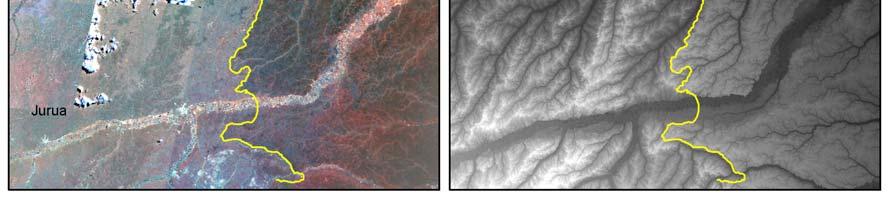
146 126

147 Figure 8: Boundary between Miocene and Late Miocene Pleistocene sediments, relative to continent scale SRTM and Landsat mosaics. Boundary is indicated by yellow line and divides dissected Miocene Pebas sediments in the west from planar Late Miocene Pleistocene sediments in the east. (A), SRTM digital elevation model for Amazonia. Light tones indicate higher elevation and dark tones lower elevation. Green box indicates the extent of figure 7, blue box indicates the extent of figures 2B and C, and inset indicates location relative to South America. (B), Landsat mosaic for the area indicated by blue box in A, with major rivers labeled. (C) SRTM digital elevation model for the same area for same area as B. Maximum and minimum elevations in A are 6157m and 0m, and in C are 779m and approximately 40m. 127

148 Figure 9: Landsat data used for Figure 7. Black outlines represent image areas, and red outline indicates mosaic area. Top value for each image indicates path and row combination for the image, and bottom value indicates day, month, and year. 128

149 Figure 10: Landsat data used for Figure 8. Black outlines represent image areas, and red outline indicates mosaic area. Top value for each image indicates path and row combination for the image, and bottom value indicates day, month, and year. 129

150 Chapter 5. Geological control of floristic composition in western Amazonia Co authors: Eneas Perez, Nydia Elespuru, Alfonso Alonso (Center for Conservation Education and Sustainability, Smithsonian Institution, Washington DC, 20013, USA.) Introduction Western Amazonia contains the largest remaining tract of undisturbed tropical forest on earth, and is thus critical to international nature conservation and carbon sequestration efforts. The physical and technical challenges of access to this vast and remote area, however, have limited efforts to produce the accurate, high resolution biodiversity maps needed for conservation and development purposes (Margules and Pressey 2000, Noss et al. 1999). As a result, biological survey in western Amazonia remains in what John Terborgh has termed the stone age (Terborgh 1992). Intensive, multi taxa inventories are available for some areas (Pitman et al. 2003), but large area maps are generally based on surrogate environmental variables or expert opinion rather than field data (Dinerstein et al. 1995). Accurate map data, supported by a firm understanding of the causes of floristic patterns, are critical for both the study and conservation of Amazonian forests 130

151 It is well known that soil properties regulate floristic composition in both temperate and tropical forests. In American temperate forests, soil properties have been demonstrated to control both the composition of climax stands and the convergence of those stands during the successional process (Christensen and Peet 1984). Within the tropics, soil properties have been found to exert strong control over composition at sites ranging from central America, to southeast Asia, to the vast expanses of Amazonia (Duivenvoorden 1995, Duque et al. 2009, Honorio et al. 2009, John et al. 2007, Palmiotto et al. 2004, Phillips et al 2003, Salovaara 2004, Tuomisto et al. 2003c). Within Amazonian forests, these changes in soil properties have been argued to result in long distance and possibly abrupt changes in floristic composition, driven by the Andean orogeny (Pitman et al. 2008, Ter Steege et al. 2006). This raises the possibility that underlying geological processes may regulate floristic composition in Amazonia, and that this may provide a general model for floristic patterns in these forests (Ter Steege et al. 2006, Pitman et al. 2008, Tuomisto et al. 1995). This hypothesis has been difficult to test, however, due to a lack of large area but detailed geological, edaphic, and floristic datasets. Here we sought to study the relationship between geological formations and plant species composition in western Amazonia, and to use available data to map these patterns. It has long been thought that soils in western Amazonia reflect a transition from older, more weathered soils in eastern Amazonia, derived from the ancient Brasilian and Guyanan Cratons; to younger, richer soils in the west, derived from recent 131

152 Andean erosion (Irion 1984). This has been proposed as the main explanation for an observed west east gradient in plant family and genus composition across Amazonia (ter Steege et al. 2000, ter Steege et al. 2006, Pitman et al. 2008). Geological studies, however, have found that widespread sediments in western Amazonia (i.e. the Pebas Formation) predate those in central Amazonia (i.e. the Içá Formation) by millions of years (Räsänen et al. 1990, Rossetti et al. 2005). This inconsistency demonstrates the need to integrate geological and ecological studies in these forests. Edaphic patterns in western Amazonia reflect a complex history of deposition and erosion, dating to the Miocene and driven by the Andean orogeny. Early stages of the Andean uplift, during the early to middle Miocene (c. 25 to 12 mya), caused the formation of the Pebas embayment and the deposition of the Pebas Formation (equivalent to the Brazilian Solimões Formation). The Pebas formation is distributed across western and central Amazonia, and consists of poorly weathered and cation rich clay sediments deposited during low energy semi marine or lacustrine conditions in the early to middle Miocene (c. 25 to 12 mya; Räsänen et al. 1995, Wesselingh et al. 2002). During this time, western Amazonian forests drained predominantly towards the northwest, though a southern connection to the Atlantic has also been proposed (Hovikoski et al. 2005). Due to further uplift during the Late Miocene Pleistocene (c. 12 mya to recent), the Pebas embayment drained and was replaced by an environment dominated by 132

153 continental fluvial or deltaic deposition, during which time the drainages of the Amazonian lowlands shifted to their contemporary eastwards course (Räsänen et al. 1990, Figueredo et al. 2009, Räsänen et al. 1987). Under these high energy conditions, the Pebas Formation was overlain by sandy, easily weathered, and cation poor sediments, such as the Nauta Formation in western Amazonia and the Içá Formation in central Amazonia (Schobbenhaus et al. 2004, Rebata et al. 2006). Continued uplift during the Plio Holocene (c. 5 recent mya) has caused drainage incision along much of the Andean foreland, replacing depositional dynamics with erosion (Räsänen et al. 1992; though broad zones of deposition remain, see Räsänen et al and 1992). This has removed the more friable and cation poor Late Miocene Pleistocene deposits across much of western Amazonia, and exposed vast expanses of the buried, cation rich Pebas Formation (Räsänen et al. 1990, INGEMMET 2000, Roddaz et al. 2005). Late Miocene Pleistocene sediments are largely preserved in central Amazonia, however, where they are represented by the Içá Formation. The exposure of the Pebas Formation across western Amazonia is not complete, however, due to the uneven nature of this uplift and river incision. As a result, mesa like islands of poorer Late Miocene Pleistocene deposits remain across western Amazonia, elevated above the Miocene Pebas matrix (Figs.1, 2; Räsänen et al. 1990, INGEMMET 2000). This dichotomy between older, richer soil Pebas Formation matrix, and younger 133

154 but poorer Late Miocene Pleistocene is a defining feature of contemporary western Amazonia, but its implications for the western Amazonian biota is poorly known. Due to the strong relationship between soil properties and species composition, we hypothesize that edaphic differences between the exposed Pebas Formation and the overlaid islands of more recent sediments will be reflected in the composition of the corresponding vegetation. This would indicate that western Amazonia exhibits largescale patch matrix dynamics, with possible implications for community assembly in these forests. Furthermore, the transition through geological time scales from a landscape dominated by nutrient poor Late Miocene Pleistocene sediments, to a landscape dominated by richer Pebas sediments, could provide a powerful mechanism for evolution of the western Amazonian biota. Last, this patch matrix configuration would have obvious implications for conservation planning in western Amazonia. To study the relationship between geological and floristic patterns in western Amazonia, we used a novel combination of SRTM (Shuttle Radar Topography Mission) elevation data (Rodriguez et al. 2006), Landsat Geocover imagery (Tucker et al. 2004), and plant and soil sampling to solve the longstanding lack of geological, edaphic, and floristic data for these forests. Geological formations can be identified from the geomorphological patterns in SRTM digital elevation data (Rossetti and Valeriano 2007), and patterns in plant species composition can be identified from Landsat data (Tuomisto et al. 1995, Tuomisto et al. 2003a, Tuomisto et al. 2003b, Salovaara et al. 2005, 134

155 Thessler et al. 2005). Matched patterns in these datasets would thus indicate geological control of floristic patterns. This hypothesis can be tested by plant and soil sampling. The SRTM and Geocover datasets are particularly useful as they provide global and georectified elevation data and Landsat imagery at no cost. These methods thus offer tools that can be used in Amazonia and beyond to map patterns in poorly studied but globally important tropical forests. Methods Study area Our study site was located in northwestern Amazonia, at the headwaters of the Curaray, Arabela, and Pucacuru rivers (Figures 11 and 12; approximately W and 1.8 S). This region is exceptionally poorly known due to its extreme remoteness and lack of large rivers, and has been identified as a conservation priority by the World Wildlife Fund (Dinerstein et al. 1995). Access to sites was provided by helicopter during seismic exploration of the Bloque 39 petroleum concession. These activities did not impact the sites in which data was collected, however, and the study area represents undisturbed lowland tropical rainforest. There is no distinct dry season in this region and annual rainfall averages mm. During our study period from April through August 135

156 2008 monthly rainfall averaged 256 mm (range: mm), and monthly daytime minimum and maximum temperatures averaged 20º and 32 º C, respectively, with little variation between months. Elevation in the study area ranged from 120 to 320 meters, with a mean elevation of 200 meters. Geological maps for Peru and SRTM imagery indicate a widespread contrast in northwestern Amazonia between elevated, mesa like islands of Late Miocene Pleistocene sediments, and the surrounding and underlying Miocene Pebas Formation (INGEMMET 2000). Our study area is typical in this regard, and contains a number of islands of the Late Miocene Pleistocene Nauta formation, surrounded by the lowerelevation Pebas matrix. We sampled this area in order to collect plant and soil data from both these Nauta Formation islands and the Pebas Formation matrix. Transects were placed to avoid tree fall gaps and streams, and were not located in white sands or inundated areas such as floodplains. As such our sampling focuses on the clay, terrafirme soils that cover the majority of the Amazonian lowlands. Satellite imagery acquisition and interpretation We used Landsat Geocover imagery to identify potential floristic patterns in our study areas (Tucker et al. 2004). Imagery was downloaded from the Global Landcover Facility (GLCF, University of Maryland, USA, and used to 136

157 construct image mosaics for each of the study areas. Geocover imagery has the advantages of being publicly available and orthorectified, thus eliminating the challenge of collecting ground control points in these remote forests and greatly improving positional accuracy. These benefits make this imagery uniquely suited to studies of remote Amazonian forests by agencies for which funding is limited. Two to three images are available for each path/row combination in the Geocover dataset, and we selected the image that was either least cloudy or of the same date as neighboring images (Figure 13). As recommended by Tuomisto et al. (2003a) we used bands four, five and seven of the original Landsat images to construct our mosaics. All images were first subset to the extent of the final mosaic area and then assembled sequentially to produce the final mosaic. Image area containing clouds was removed from the northwestern corner and southwestern edge of the image for path 8, row 62 prior to mosaic construction. Once assembled, our final mosaic was processed uniformly to improve interpretability by contrast stretching and low pass spatial convolution (image smoothing), as recommended by Hill and Foody (1994) and Tuomisto et al. (1994). All of the preceding operations were conducted in Erdas Imagine v. 8.7 (Leica Geosystems GIS & Mapping LLC.). We subsequently used ArcGIS v. 9.1 (ESRI Inc.) to remove linear brightness trends from each of the final mosaic bands in order to remove the brightness trend artifact noted by Toivonen et al. (2006). For display and interpretation, bands four, 137

158 five, and seven were assigned to red, green, and blue, respectively. Image interpretation was performed manually by MH. Interpretation was first conducted solely from Landsat imagery, and SRTM imagery was then used to refine this interpretation in case of ambiguity in the Landsat imagery. We also used shuttle radar topography mission (SRTM) digital elevation data (Rodriguez et al. 2006) to identify geological boundaries in our study areas. SRTM data was downloaded from the USGS National Map Seamless Server ( and contrast stretches were applied uniformly to maps and insets to improve interpretability. To calculate the mean elevation for each transect (see below), we used ArcGIS v 9.1 to buffer the transects to 200m such that the buffers were 400m in width and 900m in length, with rounded ends. We then used ArcGIS to calculate the mean value of all SRTM pixels located within the buffers (from an average of 38 pixels per transect). These values were then used for subsequent analyses. We last used the results from CART analyses (see below) to generate maps of predicted vegetation based on our SRTM imagery. To do this we thresholded the SRTM image for the study area by the value identified in the CART analysis. Field data collection 138

159 We inventoried Pteridophytes (ferns and fern allies) and collected soils at 52 sites in the vicinity of the Rio Curaray, Peru, using 5 m by 500 m linear transects (Figure 14; Tuomisto et al. 2003a, Tuomisto et al. 2003c). Pteridophytes reveal most of the floristic pattern captured by traditional tree inventories with a much smaller time investment (Tuomisto et al. 1995, Ruokolainen et al. 1997, Ruokolainen et al. 2007). We situated these transects so as to represent the range of tones observed in our Landsat imagery, and transect placement was stratified by our initial assessment of the geological features in the study area (i.e. Nauta islands versus Pebas matrix). To conduct our plant inventories, we opened a narrow path along the center of each transect, and recorded all species we observed to 2.5m on both sides of this path as we walked the transect. Only individuals rooted within a height of 2m and with at least one leaf longer than 10cm were included in the inventories. Climbers or epiphytes with no green leaves less than 2m above ground were not included. The product of this process was presence absence data for pteridophytes. Voucher collections for all species were deposited in herbaria in Peru (AMAZ) and Finland (TUR). At three points along each transect (approximately 50m, 250m, and 450m) we also collected soil samples. Each soil sample consisted of five subsamples collected within an area of 5 x 5m and pooled in the field. Equal dry weights of the three samples were then combined to yield a single sample for each site. These samples were processed at a single laboratory (MMT Agrifood, Jokionen, Finland), and analyzed for ph; loss on 139

160 ignition (LOI; a proxy for content of organic material in the soil); concentrations of P, Al, Ca, K, Mg, and Na; and percentage of sand, silt, and clay. Data analyses The objectives of our analyses were (1) to test the association between floristic patterns and soil properties our study area; (2) to test the association between these patterns and geological formations; and (3) to use the relationships between geological formations and species composition to model species composition throughout our study area. To visualize the floristic patterns in our study area, we performed clustering analysis with our pteridophyte transects. For clustering analysis, distance matrices were calculated using the Jaccard index, and clustering groups were generated using the group averaging method (UPGMA; PC ORD v 4.41; MjM Software). We used indicator species analysis (Dufrene and Legendre 1997; species present in eight or more transects, P 0.05) to test the relationship between individual plant species and the clustering groups. We also used non metric multidimensional scaling (NMDS) to visualize plant compositional patterns in our study area, and to extract dominant compositional trends for comparison to both elevation and edaphic properties (i.e. indirect gradient analysis). 140

161 Ordination methods such as NMDS allow variations in community composition across hundreds of species to be represented in two or three axes, such that the distance between sites along these axes is representative of their differences in species composition. We chose this approach because it can reduce noise in datasets, and because it yields a small number of compositional variables for comparison to environmental variables. We specifically chose NMDS because it makes no assumptions about relationships between variables (i.e species), and in particular does not assume linear relationships between species occurrences. For our NMDS calculations, we used PC ORD (NMS; PC ORD v 4.41; MjM Software) to identify the optimum number of NMDS dimensions for our dataset; calculate a solution at this dimensionality; and apply a varimax rotation to this solution. This last step rotates the NMDS point cloud such that the dominant compositional trend is aligned with one of the ordination axes, thus facilitating comparison of these axes to environmental variables. This technique does not change the relative distances between plots in the NMDS ordination and thus does not alter the NMDS solution. The Jaccard index was used to calculate compositional distance between sites, and we ran 400 iterations total, with a stability criterion of We last calculated the correlation between distances in the ordination space, measured by Euclidean distance, and the original distance matrix, measured with the Jaccard index. This provided a measure of the percent variation in the original dataset explained by the ordination axis. 141

162 To study the relationship between species composition and soil properties, we used three approaches. We first calculated the correlation between our ordination axes and individual environmental variables using simple linear regression. For this analysis we used 12 environmental variables: ph; LOI; log transformed concentrations of P, Al, Ca, K, Mg, and Na; percentages of sand, silt, and clay; and mean elevation, as calculated from our SRTM data (see above). We additionally used the log transformed sum of four cations, Ca, MG, Na, and K, as these variables are known to covary in western Amazonian soils (Tuomisto et al. 2003a), and because this provides a single measure of soil cation concentrations. We log transformed cation concentrations in order to give greater weight to changes in cation availability at low concentrations than at high concentrations, as recommended by Phillips et al. (2003) and Tuomisto et al. (2003a). This treatment better reflects the response by plants to these nutrients than does equal treatment across concentrations. We also used mean elevation for each transect as a surrogate for geological formation. Second, to confirm the results of these analyses, we used Mantel tests (PC ORD v 4.41; MjM Software) to calculate correlations between these individual environmental variables and floristic composition. For these tests, we also included log transformed geographic distance between sites in order to measure the effects of dispersal on composition. We log transformed geographic distance, in accordance with Condit et al (2002), as this better reflects the impact of dispersal limitation on plant composition. The 142

163 Mantel test calculates the correlation between pairs of dissimilarity matrices calculated from floristic or environmental variables. Dissimilarity matrices are square and symmetric, such that each cell in a matrix represents the dissimiliarity between a pair of sites for a given variable. Dissimilarities between sites were calculated with Euclidean distance for environmental variables, and with the one complement of the Jaccard index for our Pteridophyte data. The Mantel test was then used to calculate the Pearson s correlation coefficient (r) between pairs of matrices, and the significance of this correlation was determined by 999 permutations. It is important to note that, due to a loss of information during the transformation from raw data to distance matrices, Mantel tests give lower correlation coefficients than linear regressions in cases where both can be calculated on the same data. These methods usually agree, however, on whether the correlation is significant (Legendre 2000, Tuomisto et al. 2003a). We thus expect lower correlation coefficients for our Mantel tests than linear regression against our ordination axes, and this effect may be amplified by the reduction of noise along these axes. Third, to identify the environmental variables that best explained the floristic patterns in our study area, and to calculate the amount of floristic variation explained by these variables, we used multiple regression on distance matrices. As for our Mantel tests, distance matrices for environmental variables were calculated using Euclidean distance, and the matrix for our floristic data (Pteridophyte presence absence data) was 143

164 calculated using the one complement of the Jaccard index. To construct our multiple regression models, we began with a model that included matrices for all variables, and then used stepwise backwards elimination to exclude the environmental distance matrix with the least significant contribution to floristic distance, as calculated by a permutation test with 999 permutations. This process was repeated until all variables left in the model had regression coefficients with P < 0.05 after Bonferroni correction (see Legendre et al. 1994). All multiple regressions on distance matrices were calculated with Permute 3.4 (alpha version;legendre et al. 1994). For this analysis, we included all variables used in our Mantels tests, with the exception of elevation, which does not directly control composition. We also did not initially use the log transformed sum of cations, which would be redundant with the individual cations. To study the relationship between geological formation, soil properties, and floristic composition, we used elevation as a surrogate for geological formation, and calculated simple linear regressions between elevation and floristic composition (measured by NMDS axis I as a single, continuous variable) or the soil properties identified above. To model composition in our study area on the basis of geological formation, again represented by elevation, we used the two groups identified by our clustering analysis in a CART (classification and regression tree; JMP v. 8, SAS Institute Inc.; Vayssieres et al. 2000) analysis, in order to identify the single elevation threshold that 144

165 best divided the two groups. We validated this model using a leave one out validation method (equivalent to k fold validation, with k=52), in which 51 of the 52 sites were used to identify the elevation threshold, and this was used to predict the group membership of the remaining site. The elevation threshold was then used to classify the SRTM data for our study area into the two floristic groups. We conducted similar analyses with a subset of environmental variables to identify single thresholds in those variables that might correspond to the threshold in elevation. Results Satellite image interpretation Inspection of our Landsat and SRTM imagery revealed two primary terra firme features: darker tones in our Landsat imagery corresponding to higher elevations islands; and a lighter toned, lower elevation matrix (Figures 11 and 12). We delineated these islands and matrix manually from our imagery, and from comparison to national geological maps found that they corresponded approximately to islands of the Late Miocene Pleistocene Nauta Formation, and the underlying and surrounding Pebas Formation (INGEMMET 2000, Rebata et al. 2006; Figure 25). Analysis of SRTM imagery indicates that the Curaray, Arabela, and Pucacuru rivers are removing these Nauta 145

166 Formation sediments to expose the Pebas Formation beneath, such that the Nauta Formation remains only as highlands in the interfluvial zones between these rivers. This suggests that these islands are remnants of a once widespread Nauta Formation, now greatly reduced in area. Also visible in our Landsat imagery are large expanses of varzea, or flooded forest, visible as low elevation areas of bright red tones along the Curaray, Arabela, Pucacuru, and Tigre rivers. Due to our focus on variation in terra firme forest, these patches were excluded from sampling. Also visible in our Landsat imagery was a patch of clouds in the center of our image mosaic, and this area was also excluded from sampling. Data analyses We encountered a total of 127 species of pteridophytes and an average of 30 species per transect. Clustering analysis of the plant transects produced two floristic groups, corresponding closely to the Nauta Formation islands and Pebas Formation matrix (Figure 15). The average species turnover between transects from different groups was 77% (versus 59% within; calculated as the one complement of the Jaccard index), and 66% of the fern species were significantly associated with one of the two groups (indicator species analyses, Table 14). 146

167 Cation concentrations (sum of Ca, Mg, Na, and K) at lower elevations (the Pebas Formation), were substantially greater than those at higher elevations (the Nauta Formation islands; Figure 16). On average, cation concentrations in the group of sites corresponding to the Pebas Formation were over seven times greater than in the group corresponding to the Nauta Formation (t test, P<0.0001). Overall, cation concentrations (sum of Ca, Na, Mg, and K) in the study area ranged from 0.37 to cmol[+]/kg, on the same order of magnitude as variations found across Amazonia (Table 15; Sanchez and Buol 1974, Botschek et al. 1996). NMDS ordination of our floristic data yielded two axes (Figures 17 and 18) which explained 87% of the variation in the original plant dataset. Of the variation in the original dataset, 77% was explained by axis I, and 10% by axis II. This ordination corresponded strongly with our clustering groups, which divided the ordination space into two non overlapping groups (Figure 18). Almost all of the soil variables were significantly associated with axis I of the NMDS. The four variables most strongly correlated with this axis were log transformed concentrations of Mg, Ca, and K, and percent clay (Table 16; excluding sum of cations and elevation). These correlations were confirmed by Mantel tests, in which distances calculated from concentrations of Mg, Ca, K, and percent clay and silt, correlated best with floristic distances. Correlations between axis II and environmental variables were generally not significant (P 0.01), with the exception of weak relationships with log 147

168 transformed K and percent silt. Given the small amount of floristic variation captured by this axis, and this lack of explanatory variables, we did not include it in later analyses. Backwards regression of soil variables on floristic distance yielded a model that explained 52% of floristic composition and retained log transformed concentrations of K and Mg, and percent clay. Our Mantel tests indicated a small but significant relationship (r2 = 0.04) between geographic distance and floristic composition, and adding logtransformed geographic distance to the set of initial variables resulted in a model that retained geographic distance. This model, however, explained only an additional one percent (53% total) of variation in floristic distance, indicating that dispersal limitation is relatively insignificant in the study area, and that the effects of geographic distance are due to spatial structuring of our soil variables. These analyses consistently showed strong relationships between floristic composition, and at least four variables: log transformed concentrations of Mg, Ca, and K, and percent clay. The majority of the soil variables, however, were significantly correlated with other variables (Table 17), making it difficult to identify which variable or combination of variables is responsible for compositional patterns. Generally, however, our sample sites were characterized either by high cation concentrations (Mg, Ca, K, and Na), higher ph, and higher silt content; or by low cation concentrations, high clay content, and greater quantities of organic matter (measured as LOI). These characteristics corresponded closely to the Pebas Formation and Nauta Formation 148

169 clustering groups, respectively (see Figure 18 for examples for cation concentrations and percent clay). To partially solve the problem of correlation between soil variables, we used the log transformed sum of concentrations of Ca, Mg, Na, and K as a single measure of cation availability, consistent with previous studies (Tuomisto et al. 1995, Tuomisto et al. 2003a). To test the usefulness of this measure, we repeated our regression analysis of soil properties on floristic composition with the log transformed sum of cations substituted for concentrations of Ca, Mg, Na, and K. This analysis generated a model that explained 45% of floristic variation and retained only sum of cations and percent clay as predictor variables. A multiple regression model using both sum of cations and percent clay furthermore predicted 80% of the variation along NMDS axis I. We thus concentrated the remainder of our analyses on these two variables. Individually, the log transformed sum of cations and percent clay explain 72% and 36% of variation in NMDS axis I, respectively, and 31% and 19% of floristic distances in Mantel tests (Table 16). The Nauta Formation group exhibits uniformly low cation concentrations and a wider range of clay content, while the Pebas Formation group exhibited a wide range of both cation concentration and clay content (Figures 19 and 20). Elevation was significantly correlated both with floristic composition and with these two variables, confirming that geological formation plays an important role in determining both soil properties and floristic composition. Variations in elevation 149

170 explain 36% of the variation in NMDS axis I, and 11% of floristic distance in Mantel tests (Table 16). Elevation also separates the two clustering groups, such that lower elevations correspond primarily to Pebas Formation sites and higher elevations to Nauta Formation sites (Figure 21). On average, these two groups differ in elevation by 34 meters. Variations in elevation furthermore explain 11% of the variation observed in cation concentrations and 38% of the variation in percent clay content, such that higherelevation sites in the Nauta Formation have lower cation concentrations and higher clay contents than lower elevation sites in the Pebas Formation (Figures 22 and 23). The relationship between elevation and these variables was more evident when CART analysis was used to identify the elevation, cation concentrations, or clay content that best separated the groups identified by our clustering analysis. CART analysis indicated that an elevation value of meters, a log transformed cation sum of cmol[+]/kg, and a percent clay of 59.4%, best defined the clustering groups. Classifying the transects based on these thresholds yielded very similar results: elevation defined groups differ from cation defined groups in only seven of 52 cases (86% match), and from clay defined groups in only five cases (90% match; Table 18). This indicates that this elevation threshold corresponds closely to these cation and clay thresholds. Using the elevation threshold of meters to classify our SRTM image yielded a classification that closely matched our original image interpretation, and our 150

171 floristic and edaphic data (Figure 24). This threshold was robust in our leave one out validation analysis, and repeating the CART analysis returned the same threshold in 49 of 52 cases ( meters returned in two cases, meters returned in one case). This elevation threshold correctly classified 46 of 52 transects (89%) into their clustering groups, indicating that the model constructed for our study area is reliable. Discussion Overview Our findings provide evidence for a dichotomy in northwestern Amazonia between elevated islands of nutrient poor, Late Miocene Pleistocene fluvial deposits, and the widespread and nutrient rich Miocene Pebas Formation matrix. These formations differ seven fold in soil cation concentrations and substantially in plant species composition. These patterns can be distinguished from Landsat and SRTM satellite data, and can be mapped from SRTM data alone. The existence of a patchmatrix environment in western Amazonia has substantial implications for the ecology of these forests. In addition, the evolution of these dynamics through time has implications for the diversification of the western Amazonian biota. The distinct composition of these 151

172 islands make them important targets for conservation, and the methods described here provide a means of mapping them across western Amazonia. Relationships between elevation, soils, and floristic composition Consistent with previous studies, we found strong relationships between soil properties and floristic composition in our study area (Tuomisto et al. 1995, Phillips et al. 2003, Tuomisto et al. 2003a, Tuomisto et al. 2003b, Tuomisto et al. 2003c, Salovaara et al. 2004, John et al. 2007). The most important variables were cation concentrations (and particularly concentrations of Mg, Ca, and K), and soil texture (i.e. percent clay), and these together explained a majority of the floristic variation in the study area, whether measured along ordination axes or as compositional distance. Also consistent with these prior studies (Phillips et al. 2003), geographic distance between sites has little influence on floristic composition other than spatial structuring of soil variables. This indicates that, at the distances studied here, dispersal limitation is unimportant or overwhelmed by environmental drivers. Using elevation as a surrogate for geological formation, we found that these edaphic and floristic patterns are driven by underlying geology. Changes in elevation explain up to a third of the dominant trend in floristic variation as represented by our first NMDS axis. Due to the relatively small average difference in elevation between sites 152

173 from the two floristic groups (38m), these changes in floristic composition are unlikely to be due to variations in climate. We instead we expect them to be due to variations in soil properties, and accordingly found significant relationships between elevation and both cation concentrations and clay content. These relationships provide a mechanism by which geomorphology and geological formation are translated into floristic patterns. These findings suggest a landscape composed of higher elevation islands of low cation concentrations and high clay content; and a low elevation surface of high cation concentration and low clay content. Based on interpretation of our SRTM data, and consistent with geological studies (INGEMMET 2000), we conclude that these islands represent remnants of the Late Miocene Pleistocene Nauta Formation, surrounded by the underlying Pebas Formation, and that the Nauta Formation is being removed due to Andean uplift and subsequent river incision along the Curaray, Arabela, and Pucacuru rivers. This process of incision and erosion is most advanced nearest to these rivers, and least advanced in the interfluvial zones where these islands are located. Consequently, our findings indicate that sampling exclusively along rivers, the common form of transportation in Amazonia, may be insufficient to detect the variety of geological and floristic pattern in western Amazonia. Due to the relationship between elevation, soil properties, and floristic composition, we were able to use SRTM digital elevation data to model floristic composition in our study area. The maps generated by this process are remarkably 153

174 consistent with both our edaphic and floristic data, and existing geological maps (Figure 25). These findings provide support to the combined use of SRTM and Landsat imagery to identify matched geological and floristic patterns in Amazonian forests. Due to largescale tilt across western Amazonia however, and particularly along the Andean foreland, the elevations used here cannot be used to infer floristic patterns at other sites, and likely cannot be used over large areas. We thus suggest that these methods be used on a region to region basis. Despite strong relationships between elevation and floristic composition, however, the relationship between elevation and cation concentrations is weak. This suggests that variations in cation concentrations reflect more than a simple contrast between Pebas and Nauta Formations. We offer two explanations for this discrepancy. First, erosion by the rivers in the study area does not cleanly remove Nauta sediments from higher elevations, and instead higher elevations sediments gradually slump into lower elevation drainages, from which they are then removed. This explains the very narrow range of cation concentrations at high elevations (i.e. >250 meters) and large range of cation concentrations at lower elevations. We second suggest that the change in cation concentrations from the lowerelevation sites to the higher elevation sites causes a disproportionate change in plant species composition, such that the thresholds observed in elevation, cation concentrations, and clay content, correspond to a state change in composition. This is 154

175 supported by the disproportionate changes in composition relative to cation concentrations above 250m (Figures 21 and 22); by the compositional segregation of higher elevation plots relative to lower elevation plots (Figures 17 and 18); and by large floristic variation in the high elevation Nauta group despite little change in cation concentrations (Figure 19). This implies that the cation poor, high elevation islands of the Nauta Formation have a specialized and distinct species assemblage. It may also be the case that an unmeasured environmental variable is acting above 250m to induce this large compositional response, but we cannot suggest what this variable might be. Last, contrary to our expectations, sites in the Nauta Formation were not characterized by coarse soils typical of fluvial or deltaic deposition. Instead, clay content was substantially greater in Nauta Formation sites and sand content was uncorrelated with composition throughout the study area. This indicates that cation concentrations and soil texture are uncorrelated in our study area, though we do not expect this to be generally true of Amazonian soils. It also suggests that the original Late Miocene Pleistocene depositional dynamics may have been more varied than we believed, or that these surfaces have been modified since their deposition. For example, greater recent erosion of Pebas sediments may have depleted them of clay relative to the undisturbed Nauta islands. These uncertainties emphasize the need for geological study of these formations. 155

176 Evolution of the western Amazonian biota Our findings suggest that present day floristic patterns in northwestern Amazonia reflect the transition since the late Miocene (7 mya to present) from a landscape dominated by nutrient poor Late Miocene Pleistocene fluvial or deltaic deposits, such as the Nauta Formation, to a landscape dominated by nutrient rich deposits of lacustrine or semi marine origin, such as the Pebas Formation. This transition was the result of uplift at the Andean foreland, river incision, and the gradual removal of Late Miocene Pleistocene deposits to expose the underlying Pebas Formation. During this period, Late Miocene Pleistocene deposits shrank from a widespread matrix to isolated islands; while Pebas Formation deposits grew from isolated pockets to the present day matrix. Pebas Formation sediments continue to be exposed in central Amazonia (see Chapter 4), but the eastern extent of this formation is limited by the original extent of the Pebas embayment to central Amazonia, west of Manaus (Hoorn et al. 1995, Rossetti et al. 2005). These dynamics have implications for the evolution of the western Amazonian biota, and suggest (1) that Late Miocene Pleistocene islands in western Amazonia may serve as refugia and possible centers of speciation for taxa that were widespread during the Late Miocene; and (2) that the contemporary species pool of the Pebas Formation may reflect past diversification from poor soil ancestors in previously isolated patches of 156

177 erosion and incision during the Late Miocene. The latter is consistent with the rapid Pleistocene diversification of the rich soil plant genus Inga (Richardson et al. 2001), and the mid Miocene Pleistocene evolution of clay associated Burseraceae from species associated with nutrient poor alluvial deposits (Fine et al. 2005). This is also consistent with the recent divergence of western and eastern Amazonian avian (Bates et al. 1998, Aleixo and Rossetti 2007, Ribas et al. 2009) and primate (Silva and Oren 1996) taxa. Verifying these hypotheses will required targeted sampling of taxa in both Miocene and Late Miocene Pleistocene surfaces in western Amazonia, and possibly comparison to eastern relatives. Implications for conservation planning The existence of islands of poor soils in a richer Pebas matrix in western Amazonia has substantial implications for conservation planning. Poor soil forests are absent form the Peruvian protected area system with the exception of the small Allpuhuayo Mishana preserve in northern Peru, which protects extreme white sand patches of Quaternary origin. The majority of large protected areas in Peru are instead located in southern Peru, and protect rich soil forests in the Manu, Tambopata, or Alto Purus parks. Due to their unique flora and underrepresentation in existing protected 157

178 areas, poor soil forests on Late Miocene Pleistocene sediments should be a conservation priority for the state of Peru. The recently proposed Pucacuro protected area is the best candidate for protecting these poor soils, but its current configuration is not suitable for this purpose. This reserve encompasses the watershed of the Pucacuro river, and is thus divided evenly between the rich soils of the Pebas formation in its headwaters, in our study area, and a narrow avenue of Nauta Formation poor soils along its lower reaches. We recommend that this protected area be delineated so as to include a large portion of the watershed of the Rio Nanay, and thus include large expanses of undisturbed Late Miocene Pleistocene soils represented there by the Nauta Formation. We last recommend a survey effort throughout the northern Peruvian Amazon with the objective of mapping potential poor soil islands and verifying them with ground data. The novel combination of Landsat and SRTM data demonstrated here solves a longstanding lack of floristic and geological data for these forests, and can be used across western Amazonia to rapidly identify, verify, and map the location of these islands. These maps can then be used to produce effective and compelling strategies for the protection of the full range of the western Amazonian biota. 158

179 Table 14: Results of indicator species analysis for Pteridophyte species Species IV 1 Group 2 P 3 Adiantum cayanense 25 Nauta ** Adiantum fuliginosum Nauta ** Adiantum tomentosum Nauta ** Asplenium juglandifolium Nauta NS Cyclodium meniscioides Nauta NS Danaea lepreurii Nauta NS Elaphoglossum luridum Nauta NS Lindsea guianense Nauta ** Lindsea sp Nauta ** Metaxya rostrata Nauta ** Nephrolepis sp Nauta NS Polybotrya pubens Nauta NS Selaginella sp Nauta ** Trichomanes elegans Nauta ** Triplophyllum sp Nauta ** Adiantum humile Pebas ** Adiantum obliquum 49 Pebas ** Adiantum pulvurulentum or terminatum Pebas NS Anetium citrifolium Pebas ** Asplenium auritum Pebas ** Asplenium cirrhatum Pebas ** Asplenium pearceii Pebas ** Asplenium sp Pebas NS Bolbitis lindigii Pebas ** Campyloneurum fuscosquamatum or phyllitides Pebas ** Cnemidia speciosa Pebas NS Cyathea amazonicum or sp. 1 or lasiosora Pebas NS Cyathea cuspidata 75 Pebas ** Cyathea pungens 45 Pebas ** Danae sp Pebas NS Danaea nodosa Pebas ** Didymochlaena trunculata Pebas NS Dipazium grandifolium Pebas ** Diplazium sp Pebas NS Elaphoglossum flaccidum Pebas NS Elaphoglossum raywaense Pebas ** Lindsea digitata Pebas NS Lindsea phassa 50 Pebas ** Lomagramma guianensis Pebas ** Lomariopsis japurensis Pebas ** Lomariopsis latifolia Pebas ** 159

180 Lomariopsis nigropaleata Pebas NS Microgramma fuscosquamatum Pebas ** Polybotrya caudata or Cyclodium trianae Pebas ** Polybotrya crassirhizoma Pebas ** Polybotrya osmundaceae Pebas ** Polypodium sp Pebas NS Polypodium sp Pebas ** Polypodium sp Pebas ** Polytaenium cayenense Pebas NS Saccoloma inaequale Pebas NS Salpichlaena volubulis 49 Pebas ** Selaginella exaltata Pebas ** Tectaria brauniana or sp Pebas ** Thelypteris sp Pebas ** Thelypteris sp Pebas ** Trichomanes diversifrons Pebas ** Trichomanes pinnatum Pebas NS 1 Indicator value 2 Geologically-defined group with which species was best associated 3 P-value of association; NS indicates "not significant", ** indicates P

181 Table 15: Soil properties for 52 sites in northwestern Amazonia Tr. # ph LOI P 1 Al 1 Ca 1 K 1 Mg 1 Na 1 cations 2 Sum 161 Percent clay 3 Percent silt 3 Percent sand

182 cmol[+]/kg 2 Ca+Mg+Na+K 3 Clay defined as <0.002mm diameter; silt defined as mm; sand defined as >

183 Table 16: Correlations between floristic composition and environmental variables Environmental variable 1 Axis I Axis II Squared Mantel r ph 0.34 (0.02) 0.08 LOI 0.24 (0.11) 0.10 Log P 0.20 (0.01) 0.02 Log Al 0.19 (0.08) 0.06 LogCa 0.70 (0.06) 0.27 Log Mg 0.78 (0.10) 0.40 Log Na 0.18 (0.06) 0.02 Log K Percent clay 0.36 (0.09) 0.19 Percent silt Percent sand (0.03) (0.07) (0.00) Log sum of cations 0.72 (0.07) 0.31 Elevation 0.36 (0.09) "Log" indicates base-10 logarithm transformation All values significant at P 0.01, with exception of values in parentheses 163

184 Table 17: Pairwise correlations between environmental variables 1 LOI Log P Log Al Log Ca Log K Log Mg Log Na Log sum of cations % Clay % Silt % Sand Elev. ph LOI Log P Log Al Log Ca Log K Log Mg Log Na Log sum of cations % Clay % Silt % Sand Values for cations (P, Al, Ca, K, Mg, and Na) represent base-10 transformed concentrations (cmol[+]/kg) Values in bold are significant at P

185 Table 18: Comparison of observed and predicted floristic classes Transect Classification using CART threshold 2 Clustering group 1 Elevation 3 Log sum of cations 4 % Clay 5 1 Nauta Nauta Nauta Nauta 2 Nauta Pebas Nauta Nauta 4 Nauta Nauta Nauta Nauta 19 Nauta Nauta Nauta Nauta 21 Nauta Pebas Nauta Pebas 22 Nauta Pebas Nauta Pebas 35 Nauta Nauta Nauta Nauta 37 Nauta Nauta Nauta Pebas 38 Nauta Nauta Nauta Pebas 39 Nauta Nauta Nauta Nauta 41 Nauta Nauta Nauta Nauta 44 Nauta Nauta Nauta Nauta 45 Nauta Nauta Nauta Nauta 46 Nauta Nauta Nauta Nauta 47 Nauta Nauta Nauta Nauta 52 Nauta Nauta Nauta Nauta 3 Pebas Pebas Pebas Pebas 5 Pebas Pebas Nauta Pebas 6 Pebas Pebas Pebas Pebas 7 Pebas Pebas Pebas Pebas 8 Pebas Pebas Pebas Pebas 9 Pebas Pebas Pebas Pebas 10 Pebas Pebas Nauta Pebas 11 Pebas Pebas Pebas Pebas 12 Pebas Pebas Pebas Pebas 13 Pebas Pebas Pebas Pebas 14 Pebas Pebas Pebas Pebas 15 Pebas Pebas Pebas Pebas 16 Pebas Pebas Pebas Pebas 17 Pebas Pebas Nauta Pebas 18 Pebas Pebas Pebas Pebas 20 Pebas Pebas Pebas Pebas 23 Pebas Pebas Pebas Pebas 24 Pebas Pebas Pebas Pebas 25 Pebas Pebas Pebas Pebas 26 Pebas Pebas Pebas Pebas 27 Pebas Pebas Pebas Pebas 165

186 28 Pebas Pebas Pebas Pebas 29 Pebas Pebas Pebas Pebas 30 Pebas Pebas Pebas Pebas 31 Pebas Pebas Pebas Pebas 32 Pebas Nauta Pebas Pebas 33 Pebas Pebas Pebas Pebas 34 Pebas Pebas Pebas Pebas 36 Pebas Pebas Pebas Pebas 40 Pebas Pebas Pebas Pebas 42 Pebas Pebas Pebas Pebas 43 Pebas Nauta Nauta Pebas 48 Pebas Nauta Nauta Nauta 49 Pebas Pebas Pebas Pebas 50 Pebas Pebas Pebas Pebas 51 Pebas Pebas Pebas Pebas 1 Clustering group, named by geological formation with which it is associated 2 Classification of sites based on elevation, cation concentrations, or clay content 3 Sites classified by elevation; "Nauta" indicates elevation m, "Pebas" indicates elevation < m 4 Sites classified by base-10 logarithm transformation of sum of concentrations of Ca, Mg, K, and Na; "Nauta" indicates < , "Pebas" indicates Sites classified by clay content; "Nauta" indicates percent clay 59.4, "Pebas" indicates percent clay < 59.4 Boldface indicates error in classification relative to clustering group Table sorted by clustering group, and then by transect number 166

187 Figure 11: Landsat mosaic and interpretation for study area. Mosaic consists of four overlapping images (see Figure 13) comprised of bands 4, 5, and 7, set to display in red, green, and blue, respectively. Image interpretation is overlaid in yellow. Red tones along rivers indicate swamp forests and white area in center of image represents clouds. 167

188 Figure 12: SRTM data for study area. Light tones indicate high elevations and dark tones low elevations. Image interpretation is overlaid in blue. Elevation ranges from 120 to 320 meters. 168

189 Figure 13: Landsat images used to construct Landsat mosaic. Black lines indicate image outlines and red box indicates extent of mosaic. Upper value for each image indicates path and row of image, and bottom value indicates the image date. 169

190 Figure 14: Location of plant inventories. Green points represent 52 fern inventories esatblished during Yellow lines indicate boundaries between poorsoil islands and rich soil matrix. Landsat mosaic consists of bands 4, 5, and 7, set to red, green, and blue 170

191 Figure 15: Results of clustering analysis for fern inventories. Red and blue points indicate fern inventories, classified into twogroups. Green lines indicate boundaries between poor soil islands and rich soil matrix. Map location and scale as in Figure

192 Figure 16: Cation availability at inventory sites. Circles indicate inventory sites, and diameter of circles indicates cation availability, measured as the logtransformed sum of Mg, Ca, Na, and K concentrations. Green lines indicate boundaries between poor soil islands and rich soil matrix. Map location and scale as in Figure

193 PctClay LOI LogAl PctSilt ph LogK LogMg LogCa Figure 17: NMDS ordination of floristic data and correlations with soil properties. Horizontal axis is axis I and vertical axis is axis II. Blue triangles indicate transects, and red vectors indicate strength of correlation of environmental variables with ordination axes. Vectors for Log Na and P are obscured behind Log K and ph, respectively. 173

194 Figure 18: Relationship between clustering groups, ordination axes, and two environmental variables. Horizontal axis is NMDS axis I and vertical axis is NMDS axis II. Color of points indicates clustering group (red for Nauta group, and blue for Pebas group) and diameter indicates (A, top) cation concentration (log transformed sum of Mg, Ca, K, and Na), or (B, bottom) percent clay. 174

195 R 2 = Figure 19: Regression of cation concentrations on NMDS axis I. X axis represents the log transformed sum of cation concentrations (Mg, Ca, K, and Na), and Y axis represents positions on NMDS axis I. Color of points indicates clustering group (red for Nauta group, and blue for Pebas group) and diameter indicates elevation. Y axis crosses X axis at cation threshold identified by CART analysis ( ). 175

196 R 2 = Figure 20: Regression of clay content on NMDS axis I. X axis represents percent clay, and Y axis represents positions on NMDS axis I. Color of points indicates clustering group (red for Nauta group, and blue for Pebas group) and diameter indicates elevation. Y axis crosses X axis at percent clay threshold identified by CART analysis (59.4%). 176

197 R 2 = Figure 21: Regression of elevation on NMDS axis I. X axis represents elevation, and Y axis represents positions on NMDS axis I. Color of points indicates clustering group (red for Nauta group, and blue for Pebas group) and diameter indicates cation concentration (log transformed sum of Mg, Ca, K, and Na). Y axis crosses X axis at elevation threshold identified by CART analysis ( m). 177

198 R 2 = Figure 22: Regression of elevation on cation concentration. X axis represents elevation, and Y axis represents cation concentration (log transformed sum of Mg, Ca, K, and Na). Color of points indicates clustering group (red for Nauta group, and blue for Pebas group). Y axis crosses X axis at elevation threshold identified by CART analysis ( m), and X axis crosses Y axis at cation threshold ( ). 178

199 R 2 = Figure 23: Regression of elevation on clay content. X axis represents elevation, and Y axis represents percent clay. Color of points indicates clustering group (red for Nauta group, and blue for Pebas group). Y axis crosses X axis at elevation threshold identified by CART analysis ( m), and X axis crosses Y axis at percent clay threshold (59.4%). 179

200 Figure 24: Classified SRTM for study area. Values of 1 (white) indicate areas classified by elevation as Nauta Formation forest (elevation greater than m), and values of 0 (black) indicated areas classified as Pebas Formation forest (elevation less than m). Image interpretation is overlaid in blue. 180

201 Figure 25: Relationship between floristic composition and regional geological patterns. Labeled patches represent geological formations and yellow lines indicate boundaries identified in this study. Geological formations are as follows: NQ ns = Neogene to Quaternary, Nauta superior; NQ ni = Neogene to Quaternary, Nauta inferior; N p = Neogene, Pebas; Qp al = Pleistocene alluvial deposition; Qh al = Holocene alluvial deposition.; N i = Ipururo formation (INGEMMET 2000). 181