Numerical Modelling in Geosciences. Lecture 1 Introduction and basic mathematics for PDEs

Transcription

1 Numerical Modelling in Geosciences Lecture 1 Introduction and basic mathematics for PDEs

2 Useful information Slides and exercises: download at my homepage: Textbooks: Gerya, T. Introduction to numerical geodynamic modelling. Cambridge University Press, 345 pp. (2010). Turcotte, D.L., Schubert, G. Geodynamics. Cambridge University Press, 456 pp., 2 nd edition (2002). Any trouble?: just ask + Thursday 11:00-13:00 (???) Final exam: oral discussion about: the physics behind geological/geodynamical processes. used numerical techniques. the thermo-mechanical code the student will program through the course.

3 Why numerical modelling in geosciences? 1. Most of the geological processes occur at timescales and depths such that they cannot be observed directly. Max. human timescale Accessible by drilling (max 10 km) Unaccessible

4 Why numerical modelling in geosciences? 2. Direct measurements of, for example, stress, deformation (strain rate), composition, temperature, pressure, etc., are limited to few rock samples. With numerical models we can know their distribution everywhere in our computational domain.

5 Why numerical modelling in geosciences? 3. Numerical modelling is an indispensable tool to understand the evolution of complex geological systems together with laboratory experiments (input) and field and geophysical observations (output). Field and geophysical data Analogue/numerical modeling Understanding geological processes Lab. analysis/experiments and theory

6 What is numerical modelling in geosciences? Fundamental PDEs in this course Discretization: FD,FE,FV Eulerian+Lagrangian meshes v = 0 Conservation of mass for incompressible media σ # P = ρg Conservation of momentum for slowly flowing continuous media ρc P DT Dt = q + H Conservation of energy To close the system we need rock physical properties from lab. experiments: density thermal conductivity, expansivity heat capacity rock mechanical properties melting/metamorphic reactions

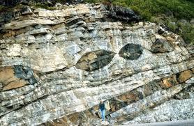
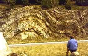
7 2D mechanical models Boudinage Buckling/folding

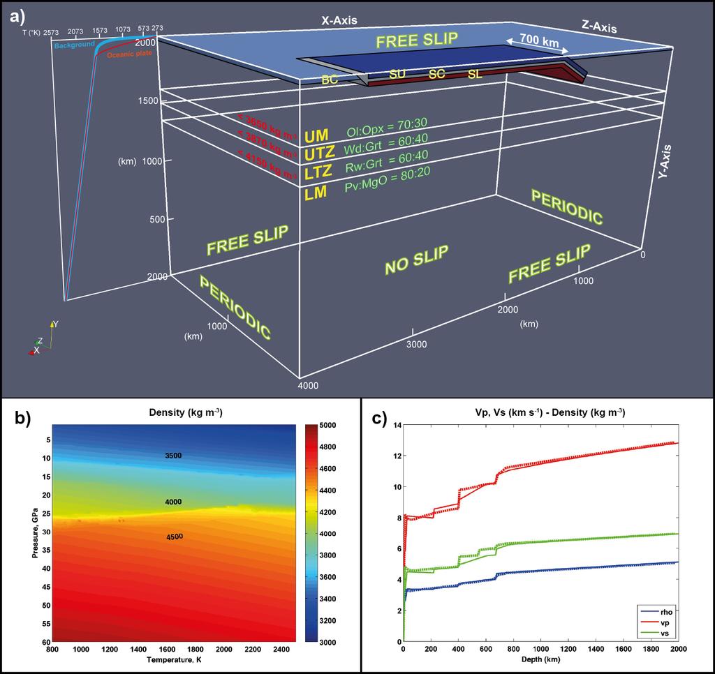
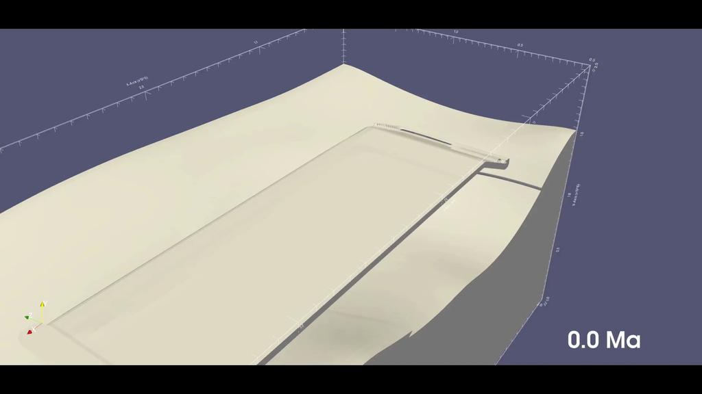
8 3D petrological-thermomechanical models 3D subduction + patterns of deformation

9 Visualization is important! Sibylla von Cleve als Braut, Lukas Cranach d. Ä. ( ) Noble dame, 1959 Succession Picasso / VG Bild-Kunst, Bonn 20

10 6.00E E E E E E E E E E+03Numerical 9.00E E+00 modeling 1.10E-09without -1.49E-09 visualization E E E E E E E E E E E E E E E E E E E E E E E E E E E E E E E E E E E E E E E E E E E E E E E E E E E E E E E E E E E E E E E E E E E E E E E E E E E E E E E E E E E E E E E E E E E E E E E E E E E E E E E E E E E E E E E E E E E E E E E E E E E E E E E E E E E E E E E E E E E E E E E E E E E E E E E E E E E E E E E E E E E E E E E E E E E E E E E E E E E E E E E E E E E E E E E E E E E E E E E E E E E E E E E E E E E E E E E E E E E E E E E E E E E E E E E E E E E E E E E E E E E E E E E E E E E E E E E E E E E E E E E E E E E E E E E E E E E E E E E E E E E E E E E E E E E E E E E E E E E E E E E E E E E E E E E E E E E E E E E E E E E E E E E E E E E E E E E E E E E E E E E E E E E E E E E E E E E E E E E E E E E E E E E E E E E E E E E E E E E E E E E E E E E E E E E E E E E E E E E E E E E E E E E E E E E E E E E E E E E E E E E E E E E E E E E E E E E E E E E E E E E E E E E E E E E E E E E+03

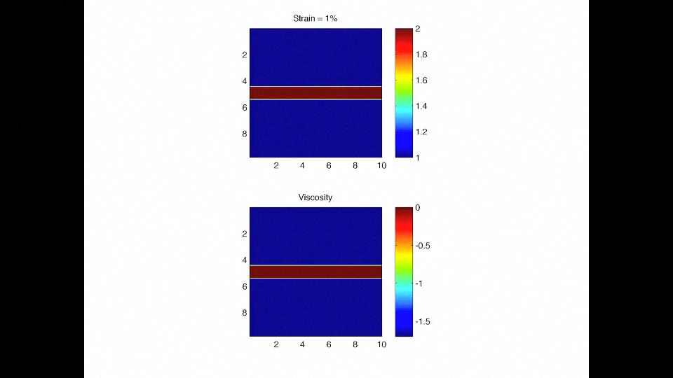
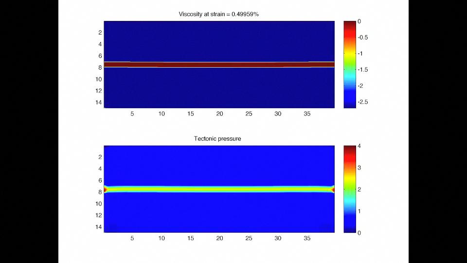
11 Numerical modeling with visualization 400 o C 800 o C 1200 o C Temperature Viscosity 200 o C 400 o C 600 o C 800 o C 1000 o C 1200 o C Bulk Strain

12 Computational resources 1D/2D models: computation and visualization can be mostly done on local machines with moderate to high RAM and 1 to 8 CPUs (depending on the numerical resolution = problem size)( ) 3D models: computation on supercomputing clusters (e.g., PLX, EURORA and FERMI at CINECA, Italy) with 100s to s CPUs. If many users, problems may arise due to long queuing times. alternatively, with about it is possible to buy medium size clusters (e.g., CPUs) that could serve the whole department. visualization requires powerful GPUs ( ) and can be done on local machines or remotely using cluster s GPUs. Workstation FERMI at CINECA, Bologna, Italy Programming languages: C/C++, Fortran, MatLab ( à Octave for free!) Visualization softwares: MatLab, Paraview, Amira, etc. This is not a coffee vending machine!

13 end of the introduction and now action

14 Mathematics First of all: it is simple!!! First and second order derivatives. (Very short) review of the mathematical background needed in this course to handle partial differential equations (PDE): differential equations in which an unknown function is a function of multiple (rather than single) independent variables (space coordinates and time). Example: 3D Heat diffusion equation à T t = k " T 2 x + T 2 2 y + T % $ 2 ' # 2 z 2 In this course we will use the finite difference method to operate differentiation and numerically solve for PDEs

15 Finite difference method First derivative of function f(x) (1D case): Example: ( ) f!( x) = f x x lim Δx 0 ( ) f ( x) (x + Δx) ( x) f x + Δx T x ΔT Δx = T T 2 1 x 2 x 1 Analytical vs Numerical T 1 " $ # T x % ' x 1 x 2 T 2 x Δx The same is valid for first derivative in time: T t ΔT Δt = T t+δt T t Δt

16 PDEs in this course and field variables Continuum mechanics PDEs v = 0 Conservation of mass for incompressible media σ # P = ρg Conservation of momentum for slowly flowing continuous media ρc P DT Dt = q + H Conservation of energy The unknown function upon which differentiation is operated describes a given field variable. Field variables describe the physical properties of the medium. Input field variables: viscosity, density, heat capacity, thermal conductivity, initial temperature field, etc. Output field variables: velocity, temperature, pressure, stress, strain rate There are 3 major types of field variables: Scalars Vectors Tensors

17 Scalar It is a number indicating the magnitude of a physical quantity, independent of the coordinate system (invariant) à pressure (P), temperature (T), density (ρ) and many other rock physical properties Gradient (gives a vector): # = x ; y ; % ( $ z' where del= is a vector differential operator Laplacian (gives a scalar): # grad(t ) = T = T x ; T y ; T % ( $ z ' T ΔT = T = 2 T = 2 x + T 2 2 y + T 2 2 z 2 % Δ = = 2 = 2 x y + ( ' 2 * 2 z 2 ) where is the Laplace operator

18 Vector It has a magnitude (length) and direction, the physical quantity is split into its components à velocity ( ), heat flux ( ), gravity ( ) Magnitude (invariant): (or Euclidean norm) Divergence (gives a scalar, invariant): where: Divergence of a vector represents the extent to which there is incoming or outgoing flux of a given physical quantity: div(v) < 0 : sink div(v) = 0 : neutral div(v) > 0 : source v $ = x + y + ' ) % z( q v = v x2 + v y2 + v z 2 g v i =! # # # " v x v y v z $ % div( v) = v = v x x + v y y + v z z

19 Vector Gradient of a vector (gives a matrix, called Jacobian): v = v i j = # % % % % % % % $ v x x v y x v z x v x y v y y v z y v x z v y z v z z ( ( ( ( ( ( ( '

20 Vector Curl (gives a vector): its magnitude expresses the amount of rotation, while its direction is normal to the plane of rotation (using the right-hand rule). curl( v) = v = 0 z z y y 0 x 0 x % ' ' ' v x v y v z ( * + * = v z * y v y -, z ) v x / z v z -, x v y / x v x -, y. 0 / Vorticity: ω = 1 2 v Product rule (Leibniz s law): Example: divergence of mass flux à Chain rule: a x = a b b x ( a b) " = a" b + b" a a or t = a x ( ) = ( ρv ) = ρ v + v ρ div ρv x t + a y y t

21 Tensor σ Stress ( ), strain ( ), strain rate ( ) ε Invariants (quantities independent of the coordinate system): - First invariant à trace:! σ xx σ xy σ xz $ # σ ij = # σ yx σ yy σ yz # " σ zx σ zy σ zz % - Second invariant à magnitude: - Third invariant à determinant ε tr( σ ) ij = ( σ xx +σ yy +σ ) zz σ = 1 σ 2 ij2 = 1 σ 2 ( 2 xx +σ 2 xy +σ 2 xz +σ 2 yx +σ 2 yy +σ 2 yz +σ 2 zx +σ 2 2 zy +σ ) zz

22 Tensor Divergence (gives a vector): σ ij = σ ij j $ = % x + σ xy y + σ ' xz ) z ) x + σ yy y + σ ) yz ) z ) x + σ zy y + σ ) zz ) z ( σ xx σ yx σ zx

23 Exercise Write the following equations using partial derivatives in 2D: v = 0 Conservation of mass for incompressible media σ # P = ρg Conservation of momentum for slowly flowing continuous media ρc P DT Dt = q + H # grad( f ) = f = f x ; f y ; f % ( $ z ' div( f ) = f = f x x + f y y + f z z Conservation of energy f ij = f ij j = $ % f xx x + f xy y + f xz z f yx x + f yy y + f yz z f zx x + f zy y + f zz z ' ) ) ) ) ) ) ) (

24 Few other rules Product rule (Leibniz s law): ( f (x) g(x) ) " = f (x)" g(x)+ g(x )" f (x) Example: divergence of mass flux à div( ρv ) = ( ρv ) = ρ v + v ρ Chain rule: df (x) dt = f (x) x dx dt or df (x, y) dt = f (x, y) x dx dt + f (x, y) y dy dt Example: dρ(t, P) dt = ρ dt T dt + ρ P dp dt

25 Numerical Modelling in Geosciences Practice 1 ok, now real action!

26 Useful information Programming language software: MatLab (any version) If not available, use Octave: open source, reads MatLab scripts and uses the same programming language and API (application programming interface). Download Octave at: Download the graphical unit interface GUIOctave at: For problems related to the installation of Octave softwares, ask (only if indispensable!) to PhD candidate Luca Penasa. Access to PCs in this room: Username: faccenda Password: faccenda2013

27 What MatLab is? MATLAB is a high-level language and interactive environment for numerical computation, visualization, and programming. Using MATLAB, you can analyze data, develop algorithms, and create models and applications. It a very useful tool for beginners because many algorithms are already built in, and we can readily analyze and visualize model results. Let s check how the graphical interface is organized

28 Practice with MatLab Exercise by: using help function and manual open a script file, how to run it and debug it. comment and semicolon defining scalar, vector, matrix and perform operations with them (e.g., a+b, a- b, a*b and a.*b, a/b, a\b) (see next slide) exercise with functions exp, log, sin, sind, asin, asind, cos, tg, ctg. produce and plot 1D data (Practice 1) initialize empty arrays and matrices (i.e., a=zeros(2,1,'int8')) programming loops (for,while,end) and conditions (if,else,elseif,end, logical (~,, ) and relational (<,>,==,>=,<=,~=) operators) (Practice 1) produce and plot 2D data (Practice 1b) open,close files (fopen,fclose) (Practice 1b) save,load data in different formats (save, load, fprintf, fread, fwrite, fscanf, hdf5write, hdf5read) (Practice 1b)

29 See also:

30 Practice with MatLab Exercise by: using help function and manual open a script file, how to run it and debug it. comment and semicolon defining scalar, vector, matrix and perform operations with them (e.g., a+b, a- b, a*b and a.*b, a/b, a\b) exercise with functions exp, log, sin, sind, asin, asind, cos, tg, ctg. produce and plot 1D data (Practice 1) initialize empty arrays and matrices (i.e., a=zeros(2,1,'int8')) (see next slide) programming loops (for,while,end) and conditions (if,else,elseif,end, logical (~,, ) and relational (<,>,==,>=,<=,~=) operators) (Practice 1) produce and plot 2D data (Practice 1b) open,close files (fopen,fclose) (Practice 1b) save,load data in different formats (save, load, fprintf, fread, fwrite, fscanf, hdf5write, hdf5read) (Practice 1b)

31 Types of variables in MatLab and their storage Field type Precision Bytes Specifier in MatLab Numeric range Unsigned integers uint8 1 %u uint16 2 %u uint32 4 %u uint64 8 %lu Signed integers int8 1 %d int16 2 %d int32 4 %d int64 8 %ld Floating-point single 4 %f,%e,%g double 8 %f,%e,%g byte = 8 bits = 221 Character string char depends on the length of the string %s,%c - By default MatLab assignes to any number a double precision, i.e., maximum storage capacity. If you want to reduce the storage, you need to specify the variable precision.

32 Practice with MatLab Exercise by: using help function and manual open a script file, how to run it and debug it. comment and semicolon defining scalar, vector, matrix and perform operations with them (e.g., a+b, a- b, a*b and a.*b, a/b, a\b) exercise with functions exp, log, sin, sind, asin, asind, cos, tg, ctg. produce and plot 1D data (Practice 1) initialize empty arrays and matrices (i.e., a=zeros(2,1,'int8')) programming loops (for,while,end) and conditions (if,else,elseif,end, logical (~,, ) and relational (<,>,==,>=,<=,~=) operators) (Practice 1) produce and plot 2D data (Practice 1b) open,close files (fopen,fclose) (Practice 1b) save,load data in different formats (save, load, fprintf, fread, fwrite, fscanf, hdf5write, hdf5read) (Practice 1b)

33 Numerical Modelling in Geosciences Practice 1b

34 Call external function In a given m-script we call an external function (i.e., here we name it test_function) In a different m-script named as the external function we can perform any operation,

35 Homework To get motivated, read the Introduction chapter of textbook: Gerya, T. Introduction to numerical geodynamic modelling. Cambridge University Press, 345 pp. (2010) Exercise with MatLab/Octave functions we have seen today Study files Practice1.m and Practice1b.m