MATH 19520/51 Class 5
|
|
|
- Myron Day
- 5 years ago
- Views:
Transcription
1 MATH 19520/51 Class 5 Minh-Tam Trinh University of Chicago
2 1 Definition of partial derivatives. 2 Geometry of partial derivatives. 3 Higher derivatives. 4 Definition of a partial differential equation (PDE). 5 Cobb Douglas production function revisited.
3 Partial Derivatives What is... The partial derivative of x y with respect to x? The partial derivative of log(ab) with respect to a? The partial derivative of 1 xy+xz+yz with respect to x?
4 Partial Derivatives What is... The partial derivative of x y with respect to x? yx y 1 The partial derivative of log(ab) with respect to a? The partial derivative of 1 xy+xz+yz with respect to x?
5 Partial Derivatives What is... The partial derivative of x y with respect to x? yx y 1 The partial derivative of log(ab) with respect to a? 1 a The partial derivative of 1 xy+xz+yz with respect to x?
6 Partial Derivatives What is... The partial derivative of x y with respect to x? yx y 1 The partial derivative of log(ab) with respect to a? 1 a The partial derivative of 1 xy+xz+yz with respect to x? y+z (xy+xz+yz) 2
7 In general, let f be a function of n variables x 1,..., x n.
8 In general, let f be a function of n variables x 1,..., x n. Formally, the partial derivative of f with respect to x i is (1) lim ɛ 0 f (x 1,..., x i + ɛ,..., x n ) f (x 1,..., x i,..., x n ). ɛ Informally, it s the derivative we get by treating the other variables x 1,..., x i 1, x i+1,..., x n as constants.
9 There are several different notations for partial derivatives: (2) f x, xf, D x f, f x all mean the partial derivative of f with respect to x. Notice that we use instead of d.
10 Example If f (x, y, z) = x yz, then what is f z (e, e, e)?
11 Example If f (x, y, z) = x yz, then what is f z (e, e, e)? Use the chain rule: (3) f z = (xyz log x) z (yz ) = (x yz log x)(y z log y). Then f z (e, e, e) = (e ee log e)(e e log e) = e ee e e = e ee +e.
12 Example ( Let f (x, y) = sin x 1 + y ). Evaluate x f and y f at (x, y) = (π, 2).
13 Example ( Let f (x, y) = sin x 1 + y We compute ( ) f x = cos x (4) 1 + y ). Evaluate x f and y f at (x, y) = (π, 2). ( x ) x 1 + y = ( ) y cos x 1 + y. (5) ( ) f y = cos x 1 + y ( x ) y 1 + y ( x = (1 + y) 2 cos x 1 + y ).
14 Example ( Let f (x, y) = sin x 1 + y We compute ( ) f x = cos x (4) 1 + y ). Evaluate x f and y f at (x, y) = (π, 2). ( x ) x 1 + y = ( ) y cos x 1 + y. (5) ( ) f y = cos x 1 + y ( x ) y 1 + y ( x = (1 + y) 2 cos x 1 + y ). Thus, f x (π, 2) = 1 3 cos π 3 = 1 6 and f y(π, 2) = π 9 cos π 3 = π 18.
15 Geometry of Partial Derivatives In 1-variable calculus, df dx (a) measures the rate of change of f in the positive x-direction at a. This is the slope of the tangent line to the graph of f at a.
16 Geometry of Partial Derivatives In 1-variable calculus, df dx (a) measures the rate of change of f in the positive x-direction at a. This is the slope of the tangent line to the graph of f at a. In 2-variable calculus, f f x (a, b) and y (a, b) respectively measure the rate of change of f in the positive x- and y-directions at (a, b). These are the slopes of tangent lines to the graph of f at (a, b). Which tangent lines?
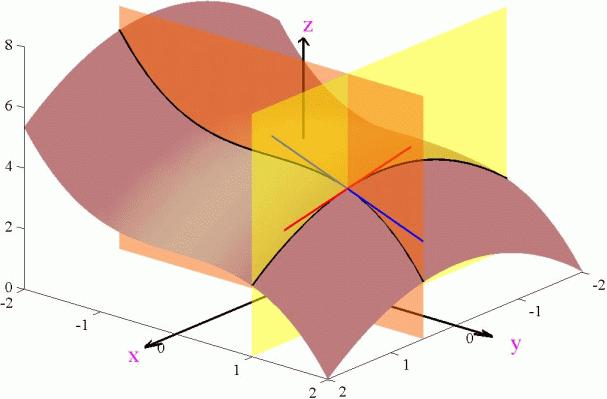
17
18 Higher Derivatives A higher derivative is when we apply several partial derivatives in succession. Stewart s notation: 2 f x 2 = ( ) f 2 f x x y x = ( ) f y x (6) and 2 f x y = ( ) f x y 2 f y 2 = ( ) f y y (7) f xx = (f x ) x f yx = (f y ) x f xy = (f x ) y f yy = (f y ) y
19 f xx, f xy, etc. are called 2 nd -order partial derivatives. In 2 variables, there are 4 kinds of 2 nd -order partial derivatives we can take: xx, xy, yx, yy.
20 f xx, f xy, etc. are called 2 nd -order partial derivatives. In 2 variables, there are 4 kinds of 2 nd -order partial derivatives we can take: xx, xy, yx, yy. In 3 variables, how many kinds of 2 nd -order partial derivatives can we take?
21 f xx, f xy, etc. are called 2 nd -order partial derivatives. In 2 variables, there are 4 kinds of 2 nd -order partial derivatives we can take: xx, xy, yx, yy. In 3 variables, how many kinds of 2 nd -order partial derivatives can we take? xx, xy, xz, yx, yy, yz, zx, zy, zz.
22 Example Find all 2 nd -order partial derivatives of f (x, y) = x 2 + 2y 2 + 3xy.
23 Example Find all 2 nd -order partial derivatives of f (x, y) = x 2 + 2y 2 + 3xy. Compute: (8) f xx = 2 f xy = 3 f yx = 3 f yy = 4 Notice that f xy = f yx.
24 Theorem (Clairaut) Let f be a differentiable function of x and y. If f x and f y exist and are continuous on a disk around (a, b), then (9) f xy (a, b) = f yx (a, b).
25 Theorem (Clairaut) Let f be a differentiable function of x and y. If f x and f y exist and are continuous on a disk around (a, b), then (9) f xy (a, b) = f yx (a, b). Warning! If f x and f y are not continuous at (0, 0), then Clairaut doesn t apply. If f (x, y) = xy(x2 y 2 ), then we can check that f x 2 +y 2 x and f y are discontinuous at (0, 0). We compute f xy (0, 0) = 1 1 = f yx (0, 0). s_theorem_where_ both_mixed_partials_are_defined_but_not_equal
26 Similarly, we can talk about 3 rd -order partial derivatives.
27 Similarly, we can talk about 3 rd -order partial derivatives. Example Find g xyz where g(x, y, z) = e xyz.
28 Similarly, we can talk about 3 rd -order partial derivatives. Example Find g xyz where g(x, y, z) = e xyz. Compute z ( y ( x (e xyz ))) = z ( y (e xyz yz)) (10)
29 Similarly, we can talk about 3 rd -order partial derivatives. Example Find g xyz where g(x, y, z) = e xyz. Compute (10) z ( y ( x (e xyz ))) = z ( y (e xyz yz)) = z (e xyz xz yz + e xyz z) = z (e xyz (xyz 2 + z))
30 Similarly, we can talk about 3 rd -order partial derivatives. Example Find g xyz where g(x, y, z) = e xyz. Compute (10) z ( y ( x (e xyz ))) = z ( y (e xyz yz)) = z (e xyz xz yz + e xyz z) = z (e xyz (xyz 2 + z)) = e xyz xy (xyz 2 + z) + e xyz (2xyz + 1) = e xyz (x 2 y 2 z 2 + 3xyz + 1).
31 Partial Differential Equations A partial differential equation (PDE) is any equation involving the partial derivatives of a function. The order of the equation is the highest order among the partial derivatives involved.
32 Partial Differential Equations A partial differential equation (PDE) is any equation involving the partial derivatives of a function. The order of the equation is the highest order among the partial derivatives involved. Example Laplace s equation for a function u(x, y) is a 2 nd -order PDE: (11) u xx + u yy = 0. Think of the function u as a variable in its own right.
33 Solution to PDEs are functions, not numbers. Just as an ordinary equation can have many numbers as solutions, a PDE can have many functions as solutions.
34 Solution to PDEs are functions, not numbers. Just as an ordinary equation can have many numbers as solutions, a PDE can have many functions as solutions. Example The function u(x, y) = x solves Laplace s equation: (12) (x) xx + (x) yy = = 0. But so does u(x, y) = x 2 y 2 : (13) (x 2 y 2 ) xx + (x 2 y 2 ) yy = 2 2 = 0.
35 Cobb Douglas Revisited Recall the Cobb Douglas production function: (14) P(L, K) = bl α K 1 α.
36 Cobb Douglas Revisited Recall the Cobb Douglas production function: (14) P(L, K) = bl α K 1 α. It is a solution to the system of equations P(L, 0) = P(0, K) = 0 (15) P L = α P L P K = β P K α + β = 1 P P L is marginal productivity of labor and K capital. is marginal productivity of
37 What do these equations mean? P(L, 0) = P(0, K) = 0 P L = α P L P K = β P K α + β = 1
38 What do these equations mean? P(L, 0) = P(0, K) = 0 To be productive, you need both labor and capital. P L = α P L P K = β P K α + β = 1
39 What do these equations mean? P(L, 0) = P(0, K) = 0 P L = α P L To be productive, you need both labor and capital. The rate at which labor increases productivity is proportional to the ratio of productivity to labor. P K = β P K α + β = 1
40 What do these equations mean? P(L, 0) = P(0, K) = 0 P L = α P L P K = β P K To be productive, you need both labor and capital. The rate at which labor increases productivity is proportional to the ratio of productivity to labor. The rate at which capital increases productivity is proportional to the ratio of productivity to capital. α + β = 1
41 What do these equations mean? P(L, 0) = P(0, K) = 0 P L = α P L P K = β P K α + β = 1 To be productive, you need both labor and capital. The rate at which labor increases productivity is proportional to the ratio of productivity to labor. The rate at which capital increases productivity is proportional to the ratio of productivity to capital. We want scaling factors to work: P(aL, ak) = ap(l, K).
MATH 19520/51 Class 4
 MATH 19520/51 Class 4 Minh-Tam Trinh University of Chicago 2017-10-02 1 Functions and independent ( nonbasic ) vs. dependent ( basic ) variables. 2 Cobb Douglas production function and its interpretation.
14.3 Partial Derivatives
 14 14.3 Copyright Cengage Learning. All rights reserved. Copyright Cengage Learning. All rights reserved. On a hot day, extreme humidity makes us think the temperature is higher than it really is, whereas
Chain Rule. MATH 311, Calculus III. J. Robert Buchanan. Spring Department of Mathematics
 3.33pt Chain Rule MATH 311, Calculus III J. Robert Buchanan Department of Mathematics Spring 2019 Single Variable Chain Rule Suppose y = g(x) and z = f (y) then dz dx = d (f (g(x))) dx = f (g(x))g (x)
Functions of Several Variables
 Functions of Several Variables Partial Derivatives Philippe B Laval KSU March 21, 2012 Philippe B Laval (KSU) Functions of Several Variables March 21, 2012 1 / 19 Introduction In this section we extend
g(t) = f(x 1 (t),..., x n (t)).
 = f(x 1 (t),..., x n (t)).") Reading: [Simon] p. 313-333, 833-836. 0.1 The Chain Rule Partial derivatives describe how a function changes in directions parallel to the coordinate axes. Now we shall demonstrate how the partial derivatives
Reading: [Simon] p. 313-333, 833-836. 0.1 The Chain Rule Partial derivatives describe how a function changes in directions parallel to the coordinate axes. Now we shall demonstrate how the partial derivatives
A DARK GREY P O N T, with a Switch Tail, and a small Star on the Forehead. Any
 Y Y Y X X «/ YY Y Y ««Y x ) & \ & & } # Y \#$& / Y Y X» \\ / X X X x & Y Y X «q «z \x» = q Y # % \ & [ & Z \ & { + % ) / / «q zy» / & / / / & x x X / % % ) Y x X Y $ Z % Y Y x x } / % «] «] # z» & Y X»
Lecture 10. (2) Functions of two variables. Partial derivatives. Dan Nichols February 27, 2018
 Functions of two variables. Partial derivatives. Dan Nichols February 27, 2018") Lecture 10 Partial derivatives Dan Nichols nichols@math.umass.edu MATH 233, Spring 2018 University of Massachusetts February 27, 2018 Last time: functions of two variables f(x, y) x and y are the independent
Lecture 10 Partial derivatives Dan Nichols nichols@math.umass.edu MATH 233, Spring 2018 University of Massachusetts February 27, 2018 Last time: functions of two variables f(x, y) x and y are the independent
Sec. 14.3: Partial Derivatives. All of the following are ways of representing the derivative. y dx
 Math 2204 Multivariable Calc Chapter 14: Partial Derivatives I. Review from math 1225 A. First Derivative Sec. 14.3: Partial Derivatives 1. Def n : The derivative of the function f with respect to the
Complex Variables. Chapter 2. Analytic Functions Section Harmonic Functions Proofs of Theorems. March 19, 2017
 Complex Variables Chapter 2. Analytic Functions Section 2.26. Harmonic Functions Proofs of Theorems March 19, 2017 () Complex Variables March 19, 2017 1 / 5 Table of contents 1 Theorem 2.26.1. 2 Theorem
Comparative Statics. Autumn 2018
 Comparative Statics Autumn 2018 What is comparative statics? Contents 1 What is comparative statics? 2 One variable functions Multiple variable functions Vector valued functions Differential and total
100 CHAPTER 4. SYSTEMS AND ADAPTIVE STEP SIZE METHODS APPENDIX
 100 CHAPTER 4. SYSTEMS AND ADAPTIVE STEP SIZE METHODS APPENDIX.1 Norms If we have an approximate solution at a given point and we want to calculate the absolute error, then we simply take the magnitude
Multivariable Calculus and Matrix Algebra-Summer 2017
 Multivariable Calculus and Matrix Algebra-Summer 017 Homework 4 Solutions Note that the solutions below are for the latest version of the problems posted. For those of you who worked on an earlier version
Limits and Continuity/Partial Derivatives
 Christopher Croke University of Pennsylvania Limits and Continuity/Partial Derivatives Math 115 Limits For (x 0, y 0 ) an interior or a boundary point of the domain of a function f (x, y). Definition:
Partial Derivatives October 2013
 Partial Derivatives 14.3 02 October 2013 Derivative in one variable. Recall for a function of one variable, f (a) = lim h 0 f (a + h) f (a) h slope f (a + h) f (a) h a a + h Partial derivatives. For a
ENGI Partial Differentiation Page y f x
 ENGI 344 4 Partial Differentiation Page 4-0 4. Partial Differentiation For functions of one variable, be found unambiguously by differentiation: y f x, the rate of change of the dependent variable can
DIFFERENTIAL EQUATIONS
 DIFFERENTIAL EQUATIONS Chapter 1 Introduction and Basic Terminology Most of the phenomena studied in the sciences and engineering involve processes that change with time. For example, it is well known
PARTIAL DERIVATIVES AND THE MULTIVARIABLE CHAIN RULE
 PARTIAL DERIVATIVES AND THE MULTIVARIABLE CHAIN RULE ADRIAN PĂCURAR LAST TIME We saw that for a function z = f(x, y) of two variables, we can take the partial derivatives with respect to x or y. For the
z 2 = 1 4 (x 2) + 1 (y 6)
 + 1 (y 6)") MA 5 Fall 007 Exam # Review Solutions. Consider the function fx, y y x. a Sketch the domain of f. For the domain, need y x 0, i.e., y x. - - - 0 0 - - - b Sketch the level curves fx, y k for k 0,,,. The
MA 5 Fall 007 Exam # Review Solutions. Consider the function fx, y y x. a Sketch the domain of f. For the domain, need y x 0, i.e., y x. - - - 0 0 - - - b Sketch the level curves fx, y k for k 0,,,. The
Example: Limit definition. Geometric meaning. Geometric meaning, y. Notes. Notes. Notes. f (x, y) = x 2 y 3 :
 = x 2 y 3 :") Partial Derivatives 14.3 02 October 2013 Derivative in one variable. Recall for a function of one variable, f (a) = lim h 0 f (a + h) f (a) h slope f (a + h) f (a) h a a + h Partial derivatives. For a
Partial Derivatives 14.3 02 October 2013 Derivative in one variable. Recall for a function of one variable, f (a) = lim h 0 f (a + h) f (a) h slope f (a + h) f (a) h a a + h Partial derivatives. For a
MA102: Multivariable Calculus
 MA102: Multivariable Calculus Rupam Barman and Shreemayee Bora Department of Mathematics IIT Guwahati Differentiability of f : U R n R m Definition: Let U R n be open. Then f : U R n R m is differentiable
MATH20411 PDEs and Vector Calculus B
 MATH2411 PDEs and Vector Calculus B Dr Stefan Güttel Acknowledgement The lecture notes and other course materials are based on notes provided by Dr Catherine Powell. SECTION 1: Introctory Material MATH2411
Module Two: Differential Calculus(continued) synopsis of results and problems (student copy)
 synopsis of results and problems (student copy)") Module Two: Differential Calculus(continued) synopsis of results and problems (student copy) Srikanth K S 1 Syllabus Taylor s and Maclaurin s theorems for function of one variable(statement only)- problems.
Module Two: Differential Calculus(continued) synopsis of results and problems (student copy) Srikanth K S 1 Syllabus Taylor s and Maclaurin s theorems for function of one variable(statement only)- problems.
2.12: Derivatives of Exp/Log (cont d) and 2.15: Antiderivatives and Initial Value Problems
 and 2.15: Antiderivatives and Initial Value Problems") 2.12: Derivatives of Exp/Log (cont d) and 2.15: Antiderivatives and Initial Value Problems Mathematics 3 Lecture 14 Dartmouth College February 03, 2010 Derivatives of the Exponential and Logarithmic Functions
2.12: Derivatives of Exp/Log (cont d) and 2.15: Antiderivatives and Initial Value Problems Mathematics 3 Lecture 14 Dartmouth College February 03, 2010 Derivatives of the Exponential and Logarithmic Functions
MATH 31BH Homework 5 Solutions
 MATH 3BH Homework 5 Solutions February 4, 204 Problem.8.2 (a) Let x t f y = x 2 + y 2 + 2z 2 and g(t) = t 2. z t 3 Then by the chain rule a a a D(g f) b = Dg f b Df b c c c = [Dg(a 2 + b 2 + 2c 2 )] [
Math 212-Lecture 8. The chain rule with one independent variable
 Math 212-Lecture 8 137: The multivariable chain rule The chain rule with one independent variable w = f(x, y) If the particle is moving along a curve x = x(t), y = y(t), then the values that the particle
Partial derivatives BUSINESS MATHEMATICS
 Partial derivatives BUSINESS MATHEMATICS 1 CONTENTS Derivatives for functions of two variables Higher-order partial derivatives Derivatives for functions of many variables Old exam question Further study
LOWELL WEEKLY JOURNAL
 Y -» $ 5 Y 7 Y Y -Y- Q x Q» 75»»/ q } # ]»\ - - $ { Q» / X x»»- 3 q $ 9 ) Y q - 5 5 3 3 3 7 Q q - - Q _»»/Q Y - 9 - - - )- [ X 7» -» - )»? / /? Q Y»» # X Q» - -?» Q ) Q \ Q - - - 3? 7» -? #»»» 7 - / Q
ENGI Partial Differentiation Page y f x
 ENGI 3424 4 Partial Differentiation Page 4-01 4. Partial Differentiation For functions of one variable, be found unambiguously by differentiation: y f x, the rate of change of the dependent variable can
Partial Derivatives for Math 229. Our puropose here is to explain how one computes partial derivatives. We will not attempt
 Partial Derivatives for Math 229 Our puropose here is to explain how one computes partial derivatives. We will not attempt to explain how they arise or why one would use them; that is left to other courses
Math Review ECON 300: Spring 2014 Benjamin A. Jones MATH/CALCULUS REVIEW
 MATH/CALCULUS REVIEW SLOPE, INTERCEPT, and GRAPHS REVIEW (adapted from Paul s Online Math Notes) Let s start with some basic review material to make sure everybody is on the same page. The slope of a line
ECON 186 Class Notes: Optimization Part 2
 ECON 186 Class Notes: Optimization Part 2 Jijian Fan Jijian Fan ECON 186 1 / 26 Hessians The Hessian matrix is a matrix of all partial derivatives of a function. Given the function f (x 1,x 2,...,x n ),
MATH The Chain Rule Fall 2016 A vector function of a vector variable is a function F: R n R m. In practice, if x 1, x n is the input,
 MATH 20550 The Chain Rule Fall 2016 A vector function of a vector variable is a function F: R n R m. In practice, if x 1, x n is the input, F(x 1,, x n ) F 1 (x 1,, x n ),, F m (x 1,, x n ) where each
Lecture 5 - Logarithms, Slope of a Function, Derivatives
 Lecture 5 - Logarithms, Slope of a Function, Derivatives 5. Logarithms Note the graph of e x This graph passes the horizontal line test, so f(x) = e x is one-to-one and therefore has an inverse function.
MATH 255 Applied Honors Calculus III Winter Homework 5 Solutions
 MATH 255 Applied Honors Calculus III Winter 2011 Homework 5 Solutions Note: In what follows, numbers in parentheses indicate the problem numbers for users of the sixth edition. A * indicates that this
Math 1314 Test 4 Review Lesson 16 Lesson Use Riemann sums with midpoints and 6 subdivisions to approximate the area between
 Math 1314 Test 4 Review Lesson 16 Lesson 24 1. Use Riemann sums with midpoints and 6 subdivisions to approximate the area between and the x-axis on the interval [1, 9]. Recall: RectangleSum[,
Lecture notes: Introduction to Partial Differential Equations
 Lecture notes: Introduction to Partial Differential Equations Sergei V. Shabanov Department of Mathematics, University of Florida, Gainesville, FL 32611 USA CHAPTER 1 Classification of Partial Differential
3 Applications of partial differentiation
 Advanced Calculus Chapter 3 Applications of partial differentiation 37 3 Applications of partial differentiation 3.1 Stationary points Higher derivatives Let U R 2 and f : U R. The partial derivatives
Lagrange Multipliers
 Optimization with Constraints As long as algebra and geometry have been separated, their progress have been slow and their uses limited; but when these two sciences have been united, they have lent each
Differentiation - Quick Review From Calculus
 Differentiation - Quick Review From Calculus Philippe B. Laval KSU Current Semester Philippe B. Laval (KSU) Differentiation - Quick Review From Calculus Current Semester 1 / 13 Introduction In this section,
Module 2: First-Order Partial Differential Equations
 Module 2: First-Order Partial Differential Equations The mathematical formulations of many problems in science and engineering reduce to study of first-order PDEs. For instance, the study of first-order
Engg. Math. I. Unit-I. Differential Calculus
 Dr. Satish Shukla 1 of 50 Engg. Math. I Unit-I Differential Calculus Syllabus: Limits of functions, continuous functions, uniform continuity, monotone and inverse functions. Differentiable functions, Rolle
e x3 dx dy. 0 y x 2, 0 x 1.
 Problem 1. Evaluate by changing the order of integration y e x3 dx dy. Solution:We change the order of integration over the region y x 1. We find and x e x3 dy dx = y x, x 1. x e x3 dx = 1 x=1 3 ex3 x=
Bessel s Equation. MATH 365 Ordinary Differential Equations. J. Robert Buchanan. Fall Department of Mathematics
 Bessel s Equation MATH 365 Ordinary Differential Equations J. Robert Buchanan Department of Mathematics Fall 2018 Background Bessel s equation of order ν has the form where ν is a constant. x 2 y + xy
LOWELL JOURNAL. MUST APOLOGIZE. such communication with the shore as Is m i Boimhle, noewwary and proper for the comfort
 - 7 7 Z 8 q ) V x - X > q - < Y Y X V - z - - - - V - V - q \ - q q < -- V - - - x - - V q > x - x q - x q - x - - - 7 -» - - - - 6 q x - > - - x - - - x- - - q q - V - x - - ( Y q Y7 - >»> - x Y - ] [
7.1 Functions of Two or More Variables
 7.1 Functions of Two or More Variables Hartfield MATH 2040 Unit 5 Page 1 Definition: A function f of two variables is a rule such that each ordered pair (x, y) in the domain of f corresponds to exactly
Neatest and Promptest Manner. E d i t u r ami rul)lihher. FOIt THE CIIILDIIES'. Trifles.
lihher. FOIt THE CIIILDIIES'. Trifles.") » ~ $ ) 7 x X ) / ( 8 2 X 39 ««x» ««! «! / x? \» «({? «» q «(? (?? x! «? 8? ( z x x q? ) «q q q ) x z x 69 7( X X ( 3»«! ( ~«x ««x ) (» «8 4 X «4 «4 «8 X «x «(» X) ()»» «X «97 X X X 4 ( 86) x) ( ) z z
» ~ $ ) 7 x X ) / ( 8 2 X 39 ««x» ««! «! / x? \» «({? «» q «(? (?? x! «? 8? ( z x x q? ) «q q q ) x z x 69 7( X X ( 3»«! ( ~«x ««x ) (» «8 4 X «4 «4 «8 X «x «(» X) ()»» «X «97 X X X 4 ( 86) x) ( ) z z
Section 3.6 The chain rule 1 Lecture. Dr. Abdulla Eid. College of Science. MATHS 101: Calculus I
 Section 3.6 The chain rule 1 Lecture College of Science MATHS 101: Calculus I (University of Bahrain) Logarithmic Differentiation 1 / 23 Motivation Goal: We want to derive rules to find the derivative
CHAPTER 4: HIGHER ORDER DERIVATIVES. Likewise, we may define the higher order derivatives. f(x, y, z) = xy 2 + e zx. y = 2xy.
 = xy 2 + e zx. y = 2xy.") April 15, 2009 CHAPTER 4: HIGHER ORDER DERIVATIVES In this chapter D denotes an open subset of R n. 1. Introduction Definition 1.1. Given a function f : D R we define the second partial derivatives as
April 15, 2009 CHAPTER 4: HIGHER ORDER DERIVATIVES In this chapter D denotes an open subset of R n. 1. Introduction Definition 1.1. Given a function f : D R we define the second partial derivatives as
DIPOLES III. q const. The voltage produced by such a charge distribution is given by. r r'
 DIPOLES III We now consider a particularly important charge configuration a dipole. This consists of two equal but opposite charges separated by a small distance. We define the dipole moment as p lim q
Two Posts to Fill On School Board
 Y Y 9 86 4 4 qz 86 x : ( ) z 7 854 Y x 4 z z x x 4 87 88 Y 5 x q x 8 Y 8 x x : 6 ; : 5 x ; 4 ( z ; ( ) ) x ; z 94 ; x 3 3 3 5 94 ; ; ; ; 3 x : 5 89 q ; ; x ; x ; ; x : ; ; ; ; ; ; 87 47% : () : / : 83
Practice problems for Exam 1. a b = (2) 2 + (4) 2 + ( 3) 2 = 29
 2 + (4) 2 + ( 3) 2 = 29") Practice problems for Exam.. Given a = and b =. Find the area of the parallelogram with adjacent sides a and b. A = a b a ı j k b = = ı j + k = ı + 4 j 3 k Thus, A = 9. a b = () + (4) + ( 3)
Practice problems for Exam.. Given a = and b =. Find the area of the parallelogram with adjacent sides a and b. A = a b a ı j k b = = ı j + k = ı + 4 j 3 k Thus, A = 9. a b = () + (4) + ( 3)
MA261-A Calculus III 2006 Fall Midterm 2 Solutions 11/8/2006 8:00AM ~9:15AM
 MA6-A Calculus III 6 Fall Midterm Solutions /8/6 8:AM ~9:5AM. Find the it xy cos y (x;y)(;) 3x + y, if it exists, or show that the it does not exist. Assume that x. The it becomes (;y)(;) y cos y 3 + y
Leplace s Equations. Analyzing the Analyticity of Analytic Analysis DEPARTMENT OF ELECTRICAL AND COMPUTER ENGINEERING. Engineering Math 16.
 Leplace s Analyzing the Analyticity of Analytic Analysis Engineering Math 16.364 1 The Laplace equations are built on the Cauchy- Riemann equations. They are used in many branches of physics such as heat
DEPARTMENT OF MATHEMATICS AND STATISTICS UNIVERSITY OF MASSACHUSETTS. MATH 233 SOME SOLUTIONS TO EXAM 2 Fall 2018
 DEPARTMENT OF MATHEMATICS AND STATISTICS UNIVERSITY OF MASSACHUSETTS MATH 233 SOME SOLUTIONS TO EXAM 2 Fall 208 Version A refers to the regular exam and Version B to the make-up. Version A. A particle
Math 212-Lecture 9. For a single-variable function z = f(x), the derivative is f (x) = lim h 0
, the derivative is f (x) = lim h 0") 3.4: Partial Derivatives Definition Mat 22-Lecture 9 For a single-variable function z = f(x), te derivative is f (x) = lim 0 f(x+) f(x). For a function z = f(x, y) of two variables, to define te derivatives,
3.4: Partial Derivatives Definition Mat 22-Lecture 9 For a single-variable function z = f(x), te derivative is f (x) = lim 0 f(x+) f(x). For a function z = f(x, y) of two variables, to define te derivatives,
Section 3.5 The Implicit Function Theorem
 Section 3.5 The Implicit Function Theorem THEOREM 11 (Special Implicit Function Theorem): Suppose that F : R n+1 R has continuous partial derivatives. Denoting points in R n+1 by (x, z), where x R n and
MECH 5312 Solid Mechanics II. Dr. Calvin M. Stewart Department of Mechanical Engineering The University of Texas at El Paso
 MECH 5312 Solid Mechanics II Dr. Calvin M. Stewart Department of Mechanical Engineering The University of Texas at El Paso Table of Contents Preliminary Math Concept of Stress Stress Components Equilibrium
Summer 2017 MATH Solution to Exercise 5
 Summer 07 MATH00 Solution to Exercise 5. Find the partial derivatives of the following functions: (a (xy 5z/( + x, (b x/ x + y, (c arctan y/x, (d log((t + 3 + ts, (e sin(xy z 3, (f x α, x = (x,, x n. (a
Differentiation of Multivariable Functions
 Differentiation of Multivariable Functions 1 Introduction Beginning calculus students identify the derivative of a function either in terms of slope or instantaneous rate of change. When thinking of the
Constrained optimization.
 ams/econ 11b supplementary notes ucsc Constrained optimization. c 2016, Yonatan Katznelson 1. Constraints In many of the optimization problems that arise in economics, there are restrictions on the values
Math 222 Spring 2013 Exam 3 Review Problem Answers
 . (a) By the Chain ule, Math Spring 3 Exam 3 eview Problem Answers w s w x x s + w y y s (y xy)() + (xy x )( ) (( s + 4t) (s 3t)( s + 4t)) ((s 3t)( s + 4t) (s 3t) ) 8s 94st + 3t (b) By the Chain ule, w
1 Arithmetic calculations (calculator is not allowed)
") 1 ARITHMETIC CALCULATIONS (CALCULATOR IS NOT ALLOWED) 1 Arithmetic calculations (calculator is not allowed) 1.1 Check the result Problem 1.1. Problem 1.2. Problem 1.3. Problem 1.4. 78 5 6 + 24 3 4 99 1
1 ARITHMETIC CALCULATIONS (CALCULATOR IS NOT ALLOWED) 1 Arithmetic calculations (calculator is not allowed) 1.1 Check the result Problem 1.1. Problem 1.2. Problem 1.3. Problem 1.4. 78 5 6 + 24 3 4 99 1
Math 1314 Lesson 23 Partial Derivatives
 Math 1314 Lesson 3 Partial Derivatives When we are asked to ind the derivative o a unction o a single variable, (x), we know exactly what to do However, when we have a unction o two variables, there is
MATH 425, FINAL EXAM SOLUTIONS
 MATH 425, FINAL EXAM SOLUTIONS Each exercise is worth 50 points. Exercise. a The operator L is defined on smooth functions of (x, y by: Is the operator L linear? Prove your answer. L (u := arctan(xy u
CHAPTER 7 DIV, GRAD, AND CURL
 CHAPTER 7 DIV, GRAD, AND CURL 1 The operator and the gradient: Recall that the gradient of a differentiable scalar field ϕ on an open set D in R n is given by the formula: (1 ϕ = ( ϕ, ϕ,, ϕ x 1 x 2 x n
2.1 NUMERICAL SOLUTION OF SIMULTANEOUS FIRST ORDER ORDINARY DIFFERENTIAL EQUATIONS. differential equations with the initial values y(x 0. ; l.
 Numerical Methods II UNIT.1 NUMERICAL SOLUTION OF SIMULTANEOUS FIRST ORDER ORDINARY DIFFERENTIAL EQUATIONS.1.1 Runge-Kutta Method of Fourth Order 1. Let = f x,y,z, = gx,y,z be the simultaneous first order
Tangent Plane. Nobuyuki TOSE. October 02, Nobuyuki TOSE. Tangent Plane
 October 02, 2017 The Equation of a plane Given a plane α passing through P 0 perpendicular to n( 0). For any point P on α, we have n PP 0 = 0 When P 0 has the coordinates (x 0, y 0, z 0 ), P 0 (x, y, z)
Lecture 13 - Wednesday April 29th
 Lecture 13 - Wednesday April 29th jacques@ucsdedu Key words: Systems of equations, Implicit differentiation Know how to do implicit differentiation, how to use implicit and inverse function theorems 131
g(2, 1) = cos(2π) + 1 = = 9
 = cos(2π) + 1 = = 9") 1. Let gx, y 2x 2 cos2πy 2 + y 2. You can use the fact that Dg2, 1 [8 2]. a Find an equation for the tangent plane to the graph z gx, y at the point 2, 1. There are two key parts to this problem. The first,
1. Let gx, y 2x 2 cos2πy 2 + y 2. You can use the fact that Dg2, 1 [8 2]. a Find an equation for the tangent plane to the graph z gx, y at the point 2, 1. There are two key parts to this problem. The first,
Math 2163, Practice Exam II, Solution
 Math 63, Practice Exam II, Solution. (a) f =< f s, f t >=< s e t, s e t >, an v v = , so D v f(, ) =< ()e, e > =< 4, 4 > = 4. (b) f =< xy 3, 3x y 4y 3 > an v =< cos π, sin π >=, so
Polynomials. In many problems, it is useful to write polynomials as products. For example, when solving equations: Example:
 Polynomials Monomials: 10, 5x, 3x 2, x 3, 4x 2 y 6, or 5xyz 2. A monomial is a product of quantities some of which are unknown. Polynomials: 10 + 5x 3x 2 + x 3, or 4x 2 y 6 + 5xyz 2. A polynomial is a
Chapter 3 Differentiation Rules
 Chapter 3 Differentiation Rules Derivative constant function if c is any real number, then Example: The Power Rule: If n is a positive integer, then Example: Extended Power Rule: If r is any real number,
MATH 19520/51 Class 11
 MATH 1952/51 Class 11 Minh-Tam Trinh University of Chicago 217-1-23 1 Discuss the midterm. 2 Review Riemann sums for functions of one variable. 3 Riemann sums for multivariable functions. 4 Double integrals
13. LECTURE 13. Objectives
 13. LECTURE 13 Objectives I can use Clairaut s Theorem to make my calculations easier. I can take higher derivatives. I can check if a function is a solution to a partial differential equation. Higher
PDE: The Method of Characteristics Page 1
 PDE: The Method of Characteristics Page y u x (x, y) + x u y (x, y) =, () u(, y) = cos y 2. Solution The partial differential equation given can be rewritten as follows: u(x, y) y, x =, (2) where = / x,
PRACTICE PROBLEMS FOR MIDTERM I
 Problem. Find the limits or explain why they do not exist (i) lim x,y 0 x +y 6 x 6 +y ; (ii) lim x,y,z 0 x 6 +y 6 +z 6 x +y +z. (iii) lim x,y 0 sin(x +y ) x +y Problem. PRACTICE PROBLEMS FOR MIDTERM I
7a3 2. (c) πa 3 (d) πa 3 (e) πa3
 πa 3 (d) πa 3 (e) πa3") 1.(6pts) Find the integral x, y, z d S where H is the part of the upper hemisphere of H x 2 + y 2 + z 2 = a 2 above the plane z = a and the normal points up. ( 2 π ) Useful Facts: cos = 1 and ds = ±a sin
1.(6pts) Find the integral x, y, z d S where H is the part of the upper hemisphere of H x 2 + y 2 + z 2 = a 2 above the plane z = a and the normal points up. ( 2 π ) Useful Facts: cos = 1 and ds = ±a sin
Homework 1/Solutions. Graded Exercises
 MTH 310-3 Abstract Algebra I and Number Theory S18 Homework 1/Solutions Graded Exercises Exercise 1. Below are parts of the addition table and parts of the multiplication table of a ring. Complete both
Contents. 2 Partial Derivatives. 2.1 Limits and Continuity. Calculus III (part 2): Partial Derivatives (by Evan Dummit, 2017, v. 2.
: Partial Derivatives (by Evan Dummit, 2017, v. 2.") Calculus III (part 2): Partial Derivatives (by Evan Dummit, 2017, v 260) Contents 2 Partial Derivatives 1 21 Limits and Continuity 1 22 Partial Derivatives 5 23 Directional Derivatives and the Gradient
Calculus III (part 2): Partial Derivatives (by Evan Dummit, 2017, v 260) Contents 2 Partial Derivatives 1 21 Limits and Continuity 1 22 Partial Derivatives 5 23 Directional Derivatives and the Gradient
Mathematical Analysis II, 2018/19 First semester
 Mathematical Analysis II, 208/9 First semester Yoh Tanimoto Dipartimento di Matematica, Università di Roma Tor Vergata Via della Ricerca Scientifica, I-0033 Roma, Italy email: hoyt@mat.uniroma2.it We basically
Leplace s Equations. Analyzing the Analyticity of Analytic Analysis DEPARTMENT OF ELECTRICAL AND COMPUTER ENGINEERING. Engineering Math EECE
 Leplace s Analyzing the Analyticity of Analytic Analysis Engineering Math EECE 3640 1 The Laplace equations are built on the Cauchy- Riemann equations. They are used in many branches of physics such as
Chapter 4. Several-variable calculus. 4.1 Derivatives of Functions of Several Variables Functions of Several Variables
 Chapter 4 Several-variable calculus 4.1 Derivatives of Functions of Several Variables 4.1.1 Functions of Several Variables ² A function f of n variables (x 1,x 2,...,x n ) in R n is an entity that operates
 «4 [< «
 The Mean Value Theorem. Oct
 The Mean Value Theorem Oct 14 2011 The Mean Value Theorem Theorem Suppose that f is defined and continuous on a closed interval [a, b], and suppose that f exists on the open interval (a, b). Then there
THE WAVE EQUATION. F = T (x, t) j + T (x + x, t) j = T (sin(θ(x, t)) + sin(θ(x + x, t)))
 j + T (x + x, t) j = T (sin(θ(x, t)) + sin(θ(x + x, t)))") THE WAVE EQUATION The aim is to derive a mathematical model that describes small vibrations of a tightly stretched flexible string for the one-dimensional case, or of a tightly stretched membrane for the
THE WAVE EQUATION The aim is to derive a mathematical model that describes small vibrations of a tightly stretched flexible string for the one-dimensional case, or of a tightly stretched membrane for the
Midterm 1 Solutions Thursday, February 26
 Math 59 Dr. DeTurck Midterm 1 Solutions Thursday, February 26 1. First note that since f() = f( + ) = f()f(), we have either f() = (in which case f(x) = f(x + ) = f(x)f() = for all x, so c = ) or else
OWELL WEEKLY JOURNAL
 Y \»< - } Y Y Y & #»»» q ] q»»»>) & - - - } ) x ( - { Y» & ( x - (» & )< - Y X - & Q Q» 3 - x Q Y 6 \Y > Y Y X 3 3-9 33 x - - / - -»- --
MANY BILLS OF CONCERN TO PUBLIC
 - 6 8 9-6 8 9 6 9 XXX 4 > -? - 8 9 x 4 z ) - -! x - x - - X - - - - - x 00 - - - - - x z - - - x x - x - - - - - ) x - - - - - - 0 > - 000-90 - - 4 0 x 00 - -? z 8 & x - - 8? > 9 - - - - 64 49 9 x - -
CALCULUS III MATH 265 FALL 2014 (COHEN) LECTURE NOTES
 LECTURE NOTES") CALCULUS III MATH 265 FALL 2014 (COHEN) LECTURE NOTES These lecture notes are intended as an outline for both student and instructor; for much more detailed exposition on the topics contained herein, the
CALCULUS III MATH 265 FALL 2014 (COHEN) LECTURE NOTES These lecture notes are intended as an outline for both student and instructor; for much more detailed exposition on the topics contained herein, the
1 Functions of Several Variables Some Examples Level Curves / Contours Functions of More Variables... 6
 Contents 1 Functions of Several Variables 1 1.1 Some Examples.................................. 2 1.2 Level Curves / Contours............................. 4 1.3 Functions of More Variables...........................
(a) The points (3, 1, 2) and ( 1, 3, 4) are the endpoints of a diameter of a sphere.
 The points (3, 1, 2) and ( 1, 3, 4) are the endpoints of a diameter of a sphere.") MATH 4 FINAL EXAM REVIEW QUESTIONS Problem. a) The points,, ) and,, 4) are the endpoints of a diameter of a sphere. i) Determine the center and radius of the sphere. ii) Find an equation for the sphere.
MATH 4 FINAL EXAM REVIEW QUESTIONS Problem. a) The points,, ) and,, 4) are the endpoints of a diameter of a sphere. i) Determine the center and radius of the sphere. ii) Find an equation for the sphere.
EconS 301. Math Review. Math Concepts
 EconS 301 Math Review Math Concepts Functions: Functions describe the relationship between input variables and outputs y f x where x is some input and y is some output. Example: x could number of Bananas
' Liberty and Umou Ono and Inseparablo "
 3 5? #< q 8 2 / / ) 9 ) 2 ) > < _ / ] > ) 2 ) ) 5 > x > [ < > < ) > _ ] ]? <
The Derivative. Appendix B. B.1 The Derivative of f. Mappings from IR to IR
 Appendix B The Derivative B.1 The Derivative of f In this chapter, we give a short summary of the derivative. Specifically, we want to compare/contrast how the derivative appears for functions whose domain
12. Stresses and Strains
 12. Stresses and Strains Finite Element Method Differential Equation Weak Formulation Approximating Functions Weighted Residuals FEM - Formulation Classification of Problems Scalar Vector 1-D T(x) u(x)
Supplementary Questions for HP Chapter Sketch graphs of the following functions: (a) z = y x. (b) z = ye x. (c) z = x 2 y 2
 z = y x. (b) z = ye x. (c) z = x 2 y 2") Supplementary Questions for HP Chapter 17 1. Sketch graphs of the following functions: (a) z = y x (b) z = ye x (c) z = x y. Find the domain and range of the given functions: (a) f(x, y) = 36 9x 4y (b)
Supplementary Questions for HP Chapter 17 1. Sketch graphs of the following functions: (a) z = y x (b) z = ye x (c) z = x y. Find the domain and range of the given functions: (a) f(x, y) = 36 9x 4y (b)
Implicit Differentiation and Inverse Trigonometric Functions
 Implicit Differentiation an Inverse Trigonometric Functions MATH 161 Calculus I J. Robert Buchanan Department of Mathematics Summer 2018 Explicit vs. Implicit Functions 0.5 1 y 0.0 y 2 0.5 3 4 1.0 0.5
Review for Exam 1. (a) Find an equation of the line through the point ( 2, 4, 10) and parallel to the vector
 Find an equation of the line through the point ( 2, 4, 10) and parallel to the vector") Calculus 3 Lia Vas Review for Exam 1 1. Surfaces. Describe the following surfaces. (a) x + y = 9 (b) x + y + z = 4 (c) z = 1 (d) x + 3y + z = 6 (e) z = x + y (f) z = x + y. Review of Vectors. (a) Let a
Calculus 3 Lia Vas Review for Exam 1 1. Surfaces. Describe the following surfaces. (a) x + y = 9 (b) x + y + z = 4 (c) z = 1 (d) x + 3y + z = 6 (e) z = x + y (f) z = x + y. Review of Vectors. (a) Let a
Differential Equations. Joe Erickson
 Differential Equations Joe Erickson Contents 1 Basic Principles 1 1.1 Functions of Several Variables.......................... 1 1.2 Linear Differential Operators........................... 7 1.3 Ordinary