Numerical Implementation of Transformation Optics
|
|
|
- Donald Baker
- 5 years ago
- Views:
Transcription
 747 6958 rcrumpf@utep.")

1 ECE st Century Electromagnetics Instructor: Office: Phone: E Mail: Dr. Raymond C. Rumpf A 337 (915) rcrumpf@utep.edu Lecture #16b Numerical Implementation of Transformation Optics Lecture 16b -- Numerical TO 1 Lecture Outline Numerical solution of Laplace s equation Calculating spatial transforms using Laplace s equation Calculating permeability and permittivity from spatial transforms Lecture 16b Numerical TO Slide 2 1
2 Numerical Solution of Laplace s Equation (Not Yet TO) Meaning of Laplace s Equation Laplace s equation is 2 u 0 2 is a 3D secondorder derivative. A second order derivative quantifies curvature. But, we set the secondorder derivative to zero. Functions satisfying Laplace s equation vary linearly. Lecture 16b Numerical TO 4 2
 Laplace s equation is solved to fill in the values away from the boundaries.")
 containing the boundary values.")
3 Laplace s Equation as a Number Filler Inner Given known values at certain points (e.g. physical boundary conditions), Laplace s equation calculates the numbers everywhere else so they vary linearly. Map of known values (boundary values) Laplace s equation is solved to fill in the values away from the boundaries. Lecture 16b Numerical TO 5 Numerical Solution of Laplace s Equation (1 of 3) Step 1 Use the finite difference method to express Laplace s equation in matrix form., u x, y u x y 2 2 u x, y 0 0 Du 2 2 x Du y 0 x y Step 2 Build a function b(x,y) containing the boundary values. bx, y b x, y This function contains the values at the locations that we wish to force u(x,y) to. The other points in b(x,y) can be set to anything, but zero is convenient. Lu 0 LD D 2 2 x y Lecture 16b Numerical TO 6 3

4 Numerical Solution of Laplace s Equation (2 of 3) Step 3 Build a diagonal force matrix. F diag f x, y This function contains 1 s at the positions where we wish to force values in u(x,y). It contains 0 s everywhere else. We set it to 1 s where we have our boundary values. f xy, Step 4 Incorporate the boundary values into Laplace s equation. L FIFL Note: both F and I should be stored as sparse matrices! b Fb Lecture 16b Numerical TO 7 Numerical Solution of Laplace s Equation (3 of 3) Step 5 Solve Laplace s equation 1 u L b The function u(x,y) has all of the forced values, but also contains all of the numbers in between. u x, y Lecture 16b Numerical TO 8 4


 of where we wish to solve")
5 Enclosed Problems Sometimes we only wish to obtain a solution that is perfectly enclosed by the boundary values. Boundary values enclose some volume. We only wish to solve Laplace s equation here. We do not care about outside of the enclosed boundary. Lecture 16b Numerical TO 9 Reducing Enclosed Problems (1 of 3) Step 1 Make a map M(x,y) of where we wish to solve Laplace s equation. b x, y M xy, Solve here. Do not solve here. Lecture 16b Numerical TO 10 5

); L =")
 Step 3 Solve Laplace s equation.")

6 Reducing Enclosed Problems (2 of 3) Step 2 Eliminate the rows and columns that correspond to points where we do not wish to solve. Lu b Lu b % REDUCE LAPLACE S EQUATION ind = find(m(:)); L = L(ind,ind); b = b(ind); Lecture 16b Numerical TO 11 Reducing Enclosed Problems (3 of 3) Step 3 Solve Laplace s equation. 1 u L b Step 4 Insert solution back into grid. % SOLVE LAPLACE'S EQUATION u = L\b; % INSERT SOLUTION BACK INTO GRID U = zeros(nx,ny); U(ind) = u; Lecture 16b Numerical TO 12 6


7 Calculating Spatial Transforms Using Laplace s Equation Step 1: Construct Object and Cloak Cloak Shape CLK Object to Cloak OBJ 0 s 1 s Lecture 16b Numerical TO 14 7
 Edge")

 External")


8 Step 2: Identify Edges of Cloak and Object (1 of 2) Edge of Cloak ECLK Edge of Object EOBJ 0 s 1 s Lecture 16b Numerical TO 15 Step 2: Identify Edges of Cloak and Object (2 of 2) External Region Object Cloak Region All edges are detected at positions outside of the cloak region. This places the edge of the object to be inside of the object. Lecture 16b Numerical TO 16 8


9 Step 3: Mask Meshgrid to Set Initial Boundary Values X F XF.* = Y F YF.* = Lecture 16b Numerical TO 17 Step 4: Force Coordinates on Object to Zero XF YF Lecture 16b Numerical TO 18 9


10 Step 5: Fill In Missing Coordinates (1 of 4) XF Solve 2 x 0 XB YF Solve 2 y 0 YB Lecture 16b Numerical TO 19 Step 5: Fill In Missing Coordinates (2 of 4) The matrix equation is constructed in three steps: Step 1/3 Construct ordinary Laplacian matrix equation. LD D 2 2 x y b column vector of forced values b x, y Step 2/3 Enforce physical boundary conditions. L FIFL b Fb Step 3/3 Eliminate don t care points. L L b b Lecture 16b Numerical TO 20 10
 Alternate view of coordinate transform: Grid Before Transform Grid After Transform Lecture 16b")
11 Step 5: Fill In Missing Coordinates (3 of 4) The matrix equation is solved in two steps: Step 1/2 Solve for u. 1 u L b Step 2/2 Insert points in u back into full grid. u u Lecture 16b Numerical TO 21 Step 5: Fill In Missing Coordinates (4 of 4) Alternate view of coordinate transform: Grid Before Transform Grid After Transform Lecture 16b Numerical TO 22 11
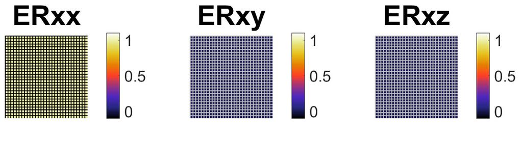

12 Calculating Permittivity and Permeability from the Spatial Transform Step 6: Initialize Background Permittivity and Permeability 1 s 0 s 0 s r r 0 s 1 s 0 s 0 s 0 s 1 s Lecture 16b Numerical TO 24 12


13 Step 7: Calculate Derivatives of Transformed Grid x Dx x x x Dx y y y Dy x x y Dy y y Lecture 16b Numerical TO 25 Step 8: Build UR and ER (1 of 4) This step loops through each point on the grid. For each point in the cloak region a. Build [ r ] and [ r ] background tensors. xx xy xz xx xy xz r yx yy yz r yx yy yz zx zy zz zx zy zz Lecture 16b Numerical TO 26 13
 This step loops through each point on the grid. For each point c.")
14 Step 8: Build UR and ER (2 of 4) This step loops through each point on the grid. For each point b. Build Jacobian. J x x 0 x y y y 0 x y Lecture 16b Numerical TO 27 Step 8: Build UR and ER (3 of 4) This step loops through each point on the grid. For each point c. Transform [ r ] and [ r ] using inverse of Jacobian. G J 1 G r G r det G T G r G r det G T % Transform UR and ER J = inv(j); UR = J*UR*J.'/det(J); ER = J*ER*J.'/det(J); Lecture 16b Numerical TO 28 14


![and [ r ].](/docs-images/83/87096865/images/15-3.jpg "xx xy xz r yx yy yz zx zy zz xx xy xz r yx yy")

15 Step 8: Build UR and ER (4 of 4) This step loops through each point on the grid. For each point d. Populate grid with transformed values of [ r ] and [ r ]. xx xy xz r yx yy yz zx zy zz xx xy xz r yx yy yz zx zy zz Lecture 16b Numerical TO 29 Step 9: Done! Numerical TO is done! The material tensors can be imported into a CEM code for simulation. r r Lecture 16b Numerical TO 30 15
Lecture #16. Spatial Transforms. Lecture 16 1
 ECE 53 1 st Century Electromagnetics Instructor: Office: Phone: E Mail: Dr. Raymond C. Rumpf A 337 (915) 747 6958 rcrumpf@utep.edu Lecture #16 Spatial ransforms Lecture 16 1 Lecture Outline ransformation
Maxwell s Equations:
 Course Instructor Dr. Raymond C. Rumpf Office: A-337 Phone: (915) 747-6958 E-Mail: rcrumpf@utep.edu Maxwell s Equations: Physical Interpretation EE-3321 Electromagnetic Field Theory Outline Maxwell s Equations
A DARK GREY P O N T, with a Switch Tail, and a small Star on the Forehead. Any
 Y Y Y X X «/ YY Y Y ««Y x ) & \ & & } # Y \#$& / Y Y X» \\ / X X X x & Y Y X «q «z \x» = q Y # % \ & [ & Z \ & { + % ) / / «q zy» / & / / / & x x X / % % ) Y x X Y $ Z % Y Y x x } / % «] «] # z» & Y X»
Electromagnetic Properties of Materials Part 2
 ECE 5322 21 st Century Electromagnetics Instructor: Office: Phone: E Mail: Dr. Raymond C. Rumpf A 337 (915) 747 6958 rcrumpf@utep.edu Lecture #3 Electromagnetic Properties of Materials Part 2 Nonlinear
Finite Element Method (FEM)
") Finite Element Method (FEM) The finite element method (FEM) is the oldest numerical technique applied to engineering problems. FEM itself is not rigorous, but when combined with integral equation techniques
Finite Element Method (FEM) The finite element method (FEM) is the oldest numerical technique applied to engineering problems. FEM itself is not rigorous, but when combined with integral equation techniques
12. Stresses and Strains
 12. Stresses and Strains Finite Element Method Differential Equation Weak Formulation Approximating Functions Weighted Residuals FEM - Formulation Classification of Problems Scalar Vector 1-D T(x) u(x)
Homework 1/Solutions. Graded Exercises
 MTH 310-3 Abstract Algebra I and Number Theory S18 Homework 1/Solutions Graded Exercises Exercise 1. Below are parts of the addition table and parts of the multiplication table of a ring. Complete both
LOWELL WEEKLY JOURNAL
 Y -» $ 5 Y 7 Y Y -Y- Q x Q» 75»»/ q } # ]»\ - - $ { Q» / X x»»- 3 q $ 9 ) Y q - 5 5 3 3 3 7 Q q - - Q _»»/Q Y - 9 - - - )- [ X 7» -» - )»? / /? Q Y»» # X Q» - -?» Q ) Q \ Q - - - 3? 7» -? #»»» 7 - / Q
MATH 19520/51 Class 5
 MATH 19520/51 Class 5 Minh-Tam Trinh University of Chicago 2017-10-04 1 Definition of partial derivatives. 2 Geometry of partial derivatives. 3 Higher derivatives. 4 Definition of a partial differential
GG303 Lecture 6 8/27/09 1 SCALARS, VECTORS, AND TENSORS
 GG303 Lecture 6 8/27/09 1 SCALARS, VECTORS, AND TENSORS I Main Topics A Why deal with tensors? B Order of scalars, vectors, and tensors C Linear transformation of scalars and vectors (and tensors) II Why
Electrostatics: Electrostatic Devices
 Electrostatics: Electrostatic Devices EE331 Electromagnetic Field Theory Outline Laplace s Equation Derivation Meaning Solving Laplace s equation Resistors Capacitors Electrostatics -- Devices Slide 1
Synthesizing Geometries for 21st Century Electromagnetics
 ECE 5322 21 st Century Electromagnetics Instructor: Office: Phone: E Mail: Dr. Raymond C. Rumpf A 337 (915) 747 6958 rcrumpf@utep.edu Lecture #18b Synthesizing Geometries for 21st Century Electromagnetics
Neatest and Promptest Manner. E d i t u r ami rul)lihher. FOIt THE CIIILDIIES'. Trifles.
lihher. FOIt THE CIIILDIIES'. Trifles.") » ~ $ ) 7 x X ) / ( 8 2 X 39 ««x» ««! «! / x? \» «({? «» q «(? (?? x! «? 8? ( z x x q? ) «q q q ) x z x 69 7( X X ( 3»«! ( ~«x ««x ) (» «8 4 X «4 «4 «8 X «x «(» X) ()»» «X «97 X X X 4 ( 86) x) ( ) z z
» ~ $ ) 7 x X ) / ( 8 2 X 39 ««x» ««! «! / x? \» «({? «» q «(? (?? x! «? 8? ( z x x q? ) «q q q ) x z x 69 7( X X ( 3»«! ( ~«x ««x ) (» «8 4 X «4 «4 «8 X «x «(» X) ()»» «X «97 X X X 4 ( 86) x) ( ) z z
Lecture Outline. Scattering at an Impedance Discontinuity Power on a Transmission Line Voltage Standing Wave Ratio (VSWR) 8/10/2018
 8/10/2018") Course Instructor Dr. Raymond C. Rumpf Office: A 337 Phone: (95) 747 6958 E Mail: rcrumpf@utep.edu EE 4347 Applied Electromagnetics Topic 4d Scattering on a Transmission Line Scattering These on a notes
Course Instructor Dr. Raymond C. Rumpf Office: A 337 Phone: (95) 747 6958 E Mail: rcrumpf@utep.edu EE 4347 Applied Electromagnetics Topic 4d Scattering on a Transmission Line Scattering These on a notes
Problem Set 2 Due Tuesday, September 27, ; p : 0. (b) Construct a representation using five d orbitals that sit on the origin as a basis: 1
 Construct a representation using five d orbitals that sit on the origin as a basis: 1") Problem Set 2 Due Tuesday, September 27, 211 Problems from Carter: Chapter 2: 2a-d,g,h,j 2.6, 2.9; Chapter 3: 1a-d,f,g 3.3, 3.6, 3.7 Additional problems: (1) Consider the D 4 point group and use a coordinate
Problem Set 2 Due Tuesday, September 27, 211 Problems from Carter: Chapter 2: 2a-d,g,h,j 2.6, 2.9; Chapter 3: 1a-d,f,g 3.3, 3.6, 3.7 Additional problems: (1) Consider the D 4 point group and use a coordinate
..«W- tn^zmxmmrrx/- NEW STORE. Popular Goods at Popular D. E. SPRING, Mas just opened a large fdo.k of DRY GOODS & GROCERIES,
 B y «X }() z zxx/ X y y y y )3 y «y
Uniformity of the Universe
 Outline Universe is homogenous and isotropic Spacetime metrics Friedmann-Walker-Robertson metric Number of numbers needed to specify a physical quantity. Energy-momentum tensor Energy-momentum tensor of
LOWELL JOURNAL. MUST APOLOGIZE. such communication with the shore as Is m i Boimhle, noewwary and proper for the comfort
 - 7 7 Z 8 q ) V x - X > q - < Y Y X V - z - - - - V - V - q \ - q q < -- V - - - x - - V q > x - x q - x q - x - - - 7 -» - - - - 6 q x - > - - x - - - x- - - q q - V - x - - ( Y q Y7 - >»> - x Y - ] [
Two Posts to Fill On School Board
 Y Y 9 86 4 4 qz 86 x : ( ) z 7 854 Y x 4 z z x x 4 87 88 Y 5 x q x 8 Y 8 x x : 6 ; : 5 x ; 4 ( z ; ( ) ) x ; z 94 ; x 3 3 3 5 94 ; ; ; ; 3 x : 5 89 q ; ; x ; x ; ; x : ; ; ; ; ; ; 87 47% : () : / : 83
Linear Algebra. Chapter 8: Eigenvalues: Further Applications and Computations Section 8.2. Applications to Geometry Proofs of Theorems.
 Linear Algebra Chapter 8: Eigenvalues: Further Applications and Computations Section 8.2. Applications to Geometry Proofs of Theorems May 1, 2018 () Linear Algebra May 1, 2018 1 / 8 Table of contents 1
COMP 175 COMPUTER GRAPHICS. Lecture 04: Transform 1. COMP 175: Computer Graphics February 9, Erik Anderson 04 Transform 1
 Lecture 04: Transform COMP 75: Computer Graphics February 9, 206 /59 Admin Sign up via email/piazza for your in-person grading Anderson@cs.tufts.edu 2/59 Geometric Transform Apply transforms to a hierarchy
' Liberty and Umou Ono and Inseparablo "
 3 5? #< q 8 2 / / ) 9 ) 2 ) > < _ / ] > ) 2 ) ) 5 > x > [ < > < ) > _ ] ]? <
Topic 8c Multi Variable Optimization
 Course Instructor Dr. Raymond C. Rumpf Office: A 337 Phone: (915) 747 6958 E Mail: rcrumpf@utep.edu Topic 8c Multi Variable Optimization EE 4386/5301 Computational Methods in EE Outline Mathematical Preliminaries
 «4 [< «
 Problem Set 2 Due Thursday, October 1, & & & & # % (b) Construct a representation using five d orbitals that sit on the origin as a basis:
 Construct a representation using five d orbitals that sit on the origin as a basis:") Problem Set 2 Due Thursday, October 1, 29 Problems from Cotton: Chapter 4: 4.6, 4.7; Chapter 6: 6.2, 6.4, 6.5 Additional problems: (1) Consider the D 3h point group and use a coordinate system wherein
Problem Set 2 Due Thursday, October 1, 29 Problems from Cotton: Chapter 4: 4.6, 4.7; Chapter 6: 6.2, 6.4, 6.5 Additional problems: (1) Consider the D 3h point group and use a coordinate system wherein
Lecture 13 - Wednesday April 29th
 Lecture 13 - Wednesday April 29th jacques@ucsdedu Key words: Systems of equations, Implicit differentiation Know how to do implicit differentiation, how to use implicit and inverse function theorems 131
MANY BILLS OF CONCERN TO PUBLIC
 - 6 8 9-6 8 9 6 9 XXX 4 > -? - 8 9 x 4 z ) - -! x - x - - X - - - - - x 00 - - - - - x z - - - x x - x - - - - - ) x - - - - - - 0 > - 000-90 - - 4 0 x 00 - -? z 8 & x - - 8? > 9 - - - - 64 49 9 x - -
DO NOT BEGIN THIS TEST UNTIL INSTRUCTED TO START
 Math 265 Student name: KEY Final Exam Fall 23 Instructor & Section: This test is closed book and closed notes. A (graphing) calculator is allowed for this test but cannot also be a communication device
M E 320 Professor John M. Cimbala Lecture 10
 M E 320 Professor John M. Cimbala Lecture 10 Today, we will: Finish our example problem rates of motion and deformation of fluid particles Discuss the Reynolds Transport Theorem (RTT) Show how the RTT
MECH 5312 Solid Mechanics II. Dr. Calvin M. Stewart Department of Mechanical Engineering The University of Texas at El Paso
 MECH 5312 Solid Mechanics II Dr. Calvin M. Stewart Department of Mechanical Engineering The University of Texas at El Paso Table of Contents Preliminary Math Concept of Stress Stress Components Equilibrium
Lecture Outline. Maxwell s Equations Predict Waves Derivation of the Wave Equation Solution to the Wave Equation 8/7/2018
 Course Instructor Dr. Raymond C. Rumpf Office: A 337 Phone: (915) 747 6958 E Mail: rcrumpf@utep.edu EE 4347 Applied Electromagnetics Topic 3a Electromagnetic Waves Electromagnetic These notes Waves may
Module 2: First-Order Partial Differential Equations
 Module 2: First-Order Partial Differential Equations The mathematical formulations of many problems in science and engineering reduce to study of first-order PDEs. For instance, the study of first-order
Rotational & Rigid-Body Mechanics. Lectures 3+4
 Rotational & Rigid-Body Mechanics Lectures 3+4 Rotational Motion So far: point objects moving through a trajectory. Next: moving actual dimensional objects and rotating them. 2 Circular Motion - Definitions
Solving Einstein s Equation Numerically III
 Solving Einstein s Equation Numerically III Lee Lindblom Center for Astrophysics and Space Sciences University of California at San Diego Mathematical Sciences Center Lecture Series Tsinghua University
OWELL WEEKLY JOURNAL
 Y \»< - } Y Y Y & #»»» q ] q»»»>) & - - - } ) x ( - { Y» & ( x - (» & )< - Y X - & Q Q» 3 - x Q Y 6 \Y > Y Y X 3 3-9 33 x - - / - -»- --
The Matrix Algebra of Sample Statistics
 The Matrix Algebra of Sample Statistics James H. Steiger Department of Psychology and Human Development Vanderbilt University James H. Steiger (Vanderbilt University) The Matrix Algebra of Sample Statistics
Multiple Integrals and Vector Calculus (Oxford Physics) Synopsis and Problem Sets; Hilary 2015
 Synopsis and Problem Sets; Hilary 2015") Multiple Integrals and Vector Calculus (Oxford Physics) Ramin Golestanian Synopsis and Problem Sets; Hilary 215 The outline of the material, which will be covered in 14 lectures, is as follows: 1. Introduction
Multiple Integrals and Vector Calculus (Oxford Physics) Ramin Golestanian Synopsis and Problem Sets; Hilary 215 The outline of the material, which will be covered in 14 lectures, is as follows: 1. Introduction
L bor y nnd Union One nnd Inseparable. LOW I'LL, MICHIGAN. WLDNHSDA Y. JULY ), I8T. liuwkll NATIdiNAI, liank
, I8T. liuwkll NATIdiNAI, liank") G k y $5 y / >/ k «««# ) /% < # «/» Y»««««?# «< >«>» y k»» «k F 5 8 Y Y F G k F >«y y
G k y $5 y / >/ k «««# ) /% < # «/» Y»««««?# «< >«>» y k»» «k F 5 8 Y Y F G k F >«y y
Lecture 8 Analyzing the diffusion weighted signal. Room CSB 272 this week! Please install AFNI
 Lecture 8 Analyzing the diffusion weighted signal Room CSB 272 this week! Please install AFNI http://afni.nimh.nih.gov/afni/ Next lecture, DTI For this lecture, think in terms of a single voxel We re still
Topic 6a Numerical Integration
 Course Instructor Dr. Raymond C. Rumpf Office: A 337 Phone: (915) 747 6958 E Mail: rcrumpf@utep.edu Topic 6a umerical Integration EE 4386/5301 Computational Methods in EE Outline Introduction Discrete
Transmission Lines Embedded in Arbitrary Anisotropic Media
 ECE 53 1 st Century Electromagnetics Instructor: Office: Phone: E Mail: Dr. Raymond C. Rumpf A 337 (915) 747 6958 rcrumpf@utep.edu Lecture #4 Transmission Lines Embedded in Arbitrary Anisotropic Media
Lecture 9 Approximations of Laplace s Equation, Finite Element Method. Mathématiques appliquées (MATH0504-1) B. Dewals, C.
 B. Dewals, C.") Lecture 9 Approximations of Laplace s Equation, Finite Element Method Mathématiques appliquées (MATH54-1) B. Dewals, C. Geuzaine V1.2 23/11/218 1 Learning objectives of this lecture Apply the finite difference
Lecture 9 Approximations of Laplace s Equation, Finite Element Method Mathématiques appliquées (MATH54-1) B. Dewals, C. Geuzaine V1.2 23/11/218 1 Learning objectives of this lecture Apply the finite difference
Getting started: CFD notation
 PDE of p-th order Getting started: CFD notation f ( u,x, t, u x 1,..., u x n, u, 2 u x 1 x 2,..., p u p ) = 0 scalar unknowns u = u(x, t), x R n, t R, n = 1,2,3 vector unknowns v = v(x, t), v R m, m =
Linear Algebra Review
 Linear Algebra Review ORIE 4741 September 1, 2017 Linear Algebra Review September 1, 2017 1 / 33 Outline 1 Linear Independence and Dependence 2 Matrix Rank 3 Invertible Matrices 4 Norms 5 Projection Matrix
Electromagnetism HW 1 math review
 Electromagnetism HW math review Problems -5 due Mon 7th Sep, 6- due Mon 4th Sep Exercise. The Levi-Civita symbol, ɛ ijk, also known as the completely antisymmetric rank-3 tensor, has the following properties:
A. H. Hall, 33, 35 &37, Lendoi
 7 X x > - z Z - ----»»x - % x x» [> Q - ) < % - - 7»- -Q 9 Q # 5 - z -> Q x > z»- ~» - x " < z Q q»» > X»? Q ~ - - % % < - < - - 7 - x -X - -- 6 97 9
Maxwell s Equations:
 Curse Instructr r. Raymnd C. Rumpf Office: A-337 Phne: (915) 747-6958 -Mail: rcrumpf@utep.edu Maxwell s quatins: Cnstitutive Relatins -3321 lectrmagnetic Field Thery Outline lectric Respnse f Materials
CSE 167: Introduction to Computer Graphics Lecture #2: Linear Algebra Primer
 CSE 167: Introduction to Computer Graphics Lecture #2: Linear Algebra Primer Jürgen P. Schulze, Ph.D. University of California, San Diego Fall Quarter 2016 Announcements Monday October 3: Discussion Assignment
AMS 147 Computational Methods and Applications Lecture 17 Copyright by Hongyun Wang, UCSC
 Lecture 17 Copyright by Hongyun Wang, UCSC Recap: Solving linear system A x = b Suppose we are given the decomposition, A = L U. We solve (LU) x = b in 2 steps: *) Solve L y = b using the forward substitution
A Brief Revision of Vector Calculus and Maxwell s Equations
 A Brief Revision of Vector Calculus and Maxwell s Equations Debapratim Ghosh Electronic Systems Group Department of Electrical Engineering Indian Institute of Technology Bombay e-mail: dghosh@ee.iitb.ac.in
EE 5337 Computational Electromagnetics (CEM) Introduction to CEM
 Introduction to CEM") Instructor Dr. Raymond Rumpf (915) 747 6958 rcrumpf@utep.edu EE 5337 Computational Electromagnetics (CEM) Lecture #1 Introduction to CEM Lecture 1These notes may contain copyrighted material obtained under
Instructor Dr. Raymond Rumpf (915) 747 6958 rcrumpf@utep.edu EE 5337 Computational Electromagnetics (CEM) Lecture #1 Introduction to CEM Lecture 1These notes may contain copyrighted material obtained under
7a3 2. (c) πa 3 (d) πa 3 (e) πa3
 πa 3 (d) πa 3 (e) πa3") 1.(6pts) Find the integral x, y, z d S where H is the part of the upper hemisphere of H x 2 + y 2 + z 2 = a 2 above the plane z = a and the normal points up. ( 2 π ) Useful Facts: cos = 1 and ds = ±a sin
1.(6pts) Find the integral x, y, z d S where H is the part of the upper hemisphere of H x 2 + y 2 + z 2 = a 2 above the plane z = a and the normal points up. ( 2 π ) Useful Facts: cos = 1 and ds = ±a sin
CHAPTER 7 DIV, GRAD, AND CURL
 CHAPTER 7 DIV, GRAD, AND CURL 1 The operator and the gradient: Recall that the gradient of a differentiable scalar field ϕ on an open set D in R n is given by the formula: (1 ϕ = ( ϕ, ϕ,, ϕ x 1 x 2 x n
Topic 7e Finite Difference Analysis of Transmission Lines
 Course Instructor r. Raymond C. Rumpf Office: A 337 Phone: (915) 747 6958 Mail: rcrumpf@utep.edu Topic 7e Finite ifference Analysis of Transmission Lines 4386/531 Computational Methods in 1 Outline Introduction
Rigid body dynamics. Basilio Bona. DAUIN - Politecnico di Torino. October 2013
 Rigid body dynamics Basilio Bona DAUIN - Politecnico di Torino October 2013 Basilio Bona (DAUIN - Politecnico di Torino) Rigid body dynamics October 2013 1 / 16 Multiple point-mass bodies Each mass is
6. SCALARS, VECTORS, AND TENSORS (FOR ORTHOGONAL COORDINATE SYSTEMS)
") (FOR ORTHOGONAL COORDINATE SYSTEMS) I Main Topics A What are scalars, vectors, and tensors? B Order of scalars, vectors, and tensors C Linear transformaoon of scalars and vectors (and tensors) D Matrix
(FOR ORTHOGONAL COORDINATE SYSTEMS) I Main Topics A What are scalars, vectors, and tensors? B Order of scalars, vectors, and tensors C Linear transformaoon of scalars and vectors (and tensors) D Matrix
Lecture 4: Least Squares (LS) Estimation
 Estimation") ME 233, UC Berkeley, Spring 2014 Xu Chen Lecture 4: Least Squares (LS) Estimation Background and general solution Solution in the Gaussian case Properties Example Big picture general least squares estimation:
ME 233, UC Berkeley, Spring 2014 Xu Chen Lecture 4: Least Squares (LS) Estimation Background and general solution Solution in the Gaussian case Properties Example Big picture general least squares estimation:
Statistics 351 Probability I Fall 2006 (200630) Final Exam Solutions. θ α β Γ(α)Γ(β) (uv)α 1 (v uv) β 1 exp v }
 Final Exam Solutions. θ α β Γ(α)Γ(β) (uv)α 1 (v uv) β 1 exp v }") Statistics 35 Probability I Fall 6 (63 Final Exam Solutions Instructor: Michael Kozdron (a Solving for X and Y gives X UV and Y V UV, so that the Jacobian of this transformation is x x u v J y y v u v
Statistics 35 Probability I Fall 6 (63 Final Exam Solutions Instructor: Michael Kozdron (a Solving for X and Y gives X UV and Y V UV, so that the Jacobian of this transformation is x x u v J y y v u v
Chapter 9: Differential Analysis
 9-1 Introduction 9-2 Conservation of Mass 9-3 The Stream Function 9-4 Conservation of Linear Momentum 9-5 Navier Stokes Equation 9-6 Differential Analysis Problems Recall 9-1 Introduction (1) Chap 5: Control
AB-267 DYNAMICS & CONTROL OF FLEXIBLE AIRCRAFT
 FLÁIO SILESTRE DYNAMICS & CONTROL OF FLEXIBLE AIRCRAFT LECTURE NOTES LAGRANGIAN MECHANICS APPLIED TO RIGID-BODY DYNAMICS IMAGE CREDITS: BOEING FLÁIO SILESTRE Introduction Lagrangian Mechanics shall be
Solution of Matrix Eigenvalue Problem
 Outlines October 12, 2004 Outlines Part I: Review of Previous Lecture Part II: Review of Previous Lecture Outlines Part I: Review of Previous Lecture Part II: Standard Matrix Eigenvalue Problem Other Forms
Maxwell s Equations:
 Course Instructor Dr. Raymond C. Rumpf Office: A-337 Phone: (915) 747-6958 E-Mail: rcrumpf@utep.edu Maxwell s Equations: Terms & Definitions EE-3321 Electromagnetic Field Theory Outline Maxwell s Equations
CSE 167: Introduction to Computer Graphics Lecture #2: Linear Algebra Primer
 CSE 167: Introduction to Computer Graphics Lecture #2: Linear Algebra Primer Jürgen P. Schulze, Ph.D. University of California, San Diego Spring Quarter 2016 Announcements Project 1 due next Friday at
Introduction and some preliminaries
 1 Partial differential equations Introduction and some preliminaries A partial differential equation (PDE) is a relationship among partial derivatives of a function (or functions) of more than one variable.
Chapter 9: Differential Analysis of Fluid Flow
 of Fluid Flow Objectives 1. Understand how the differential equations of mass and momentum conservation are derived. 2. Calculate the stream function and pressure field, and plot streamlines for a known
Wave and Elasticity Equations
 1 Wave and lasticity quations Now let us consider the vibrating string problem which is modeled by the one-dimensional wave equation. Suppose that a taut string is suspended by its extremes at the points
General Relativity ASTR 2110 Sarazin. Einstein s Equation
 General Relativity ASTR 2110 Sarazin Einstein s Equation Curvature of Spacetime 1. Principle of Equvalence: gravity acceleration locally 2. Acceleration curved path in spacetime In gravitational field,
In this section, mathematical description of the motion of fluid elements moving in a flow field is
 Jun. 05, 015 Chapter 6. Differential Analysis of Fluid Flow 6.1 Fluid Element Kinematics In this section, mathematical description of the motion of fluid elements moving in a flow field is given. A small
Electromagnetism II Lecture 7
 Electromagnetism II Lecture 7 Instructor: Andrei Sirenko sirenko@njit.edu Spring 13 Thursdays 1 pm 4 pm Spring 13, NJIT 1 Previous Lecture: Conservation Laws Previous Lecture: EM waves Normal incidence
Exercise 1: Inertia moment of a simple pendulum
 Exercise : Inertia moment of a simple pendulum A simple pendulum is represented in Figure. Three reference frames are introduced: R is the fixed/inertial RF, with origin in the rotation center and i along
6. 3D Kinematics DE2-EA 2.1: M4DE. Dr Connor Myant
 DE2-EA 2.1: M4DE Dr Connor Myant 6. 3D Kinematics Comments and corrections to connor.myant@imperial.ac.uk Lecture resources may be found on Blackboard and at http://connormyant.com Contents Three-Dimensional
Multiple Integrals and Vector Calculus: Synopsis
 Multiple Integrals and Vector Calculus: Synopsis Hilary Term 28: 14 lectures. Steve Rawlings. 1. Vectors - recap of basic principles. Things which are (and are not) vectors. Differentiation and integration
General Physics I. Lecture 10: Rolling Motion and Angular Momentum.
 General Physics I Lecture 10: Rolling Motion and Angular Momentum Prof. WAN, Xin (万歆) 万歆 ) xinwan@zju.edu.cn http://zimp.zju.edu.cn/~xinwan/ Outline Rolling motion of a rigid object: center-of-mass motion
Chapter 5. The Differential Forms of the Fundamental Laws
 Chapter 5 The Differential Forms of the Fundamental Laws 1 5.1 Introduction Two primary methods in deriving the differential forms of fundamental laws: Gauss s Theorem: Allows area integrals of the equations
Lecture 5: Random Walks and Markov Chain
 Spectral Graph Theory and Applications WS 20/202 Lecture 5: Random Walks and Markov Chain Lecturer: Thomas Sauerwald & He Sun Introduction to Markov Chains Definition 5.. A sequence of random variables
DIPOLES III. q const. The voltage produced by such a charge distribution is given by. r r'
 DIPOLES III We now consider a particularly important charge configuration a dipole. This consists of two equal but opposite charges separated by a small distance. We define the dipole moment as p lim q
Group, Rings, and Fields Rahul Pandharipande. I. Sets Let S be a set. The Cartesian product S S is the set of ordered pairs of elements of S,
 Group, Rings, and Fields Rahul Pandharipande I. Sets Let S be a set. The Cartesian product S S is the set of ordered pairs of elements of S, A binary operation φ is a function, S S = {(x, y) x, y S}. φ
Game Physics. Game and Media Technology Master Program - Utrecht University. Dr. Nicolas Pronost
 Game and Media Technology Master Program - Utrecht University Dr. Nicolas Pronost Rigid body physics Particle system Most simple instance of a physics system Each object (body) is a particle Each particle
AE/ME 339. Computational Fluid Dynamics (CFD) K. M. Isaac. Momentum equation. Computational Fluid Dynamics (AE/ME 339) MAEEM Dept.
 K. M. Isaac. Momentum equation. Computational Fluid Dynamics (AE/ME 339) MAEEM Dept.") AE/ME 339 Computational Fluid Dynamics (CFD) 9//005 Topic7_NS_ F0 1 Momentum equation 9//005 Topic7_NS_ F0 1 Consider the moving fluid element model shown in Figure.b Basis is Newton s nd Law which says
AE/ME 339 Computational Fluid Dynamics (CFD) 9//005 Topic7_NS_ F0 1 Momentum equation 9//005 Topic7_NS_ F0 1 Consider the moving fluid element model shown in Figure.b Basis is Newton s nd Law which says
LOWELL WEEKLY JOURNAL.
 Y $ Y Y 7 27 Y 2» x 7»» 2» q» ~ [ } q q $ $ 6 2 2 2 2 2 2 7 q > Y» Y >» / Y» ) Y» < Y»» _»» < Y > Y Y < )»» >» > ) >» >> >Y x x )»» > Y Y >>»» }> ) Y < >» /» Y x» > / x /»»»»» >» >» >»» > > >» < Y /~ >
AMC Lecture Notes. Justin Stevens. Cybermath Academy
 AMC Lecture Notes Justin Stevens Cybermath Academy Contents 1 Systems of Equations 1 1 Systems of Equations 1.1 Substitution Example 1.1. Solve the system below for x and y: x y = 4, 2x + y = 29. Solution.
Random Signals and Systems. Chapter 3. Jitendra K Tugnait. Department of Electrical & Computer Engineering. Auburn University.
 Random Signals and Systems Chapter 3 Jitendra K Tugnait Professor Department of Electrical & Computer Engineering Auburn University Two Random Variables Previously, we only dealt with one random variable
Artificial Intelligence & Neuro Cognitive Systems Fakultät für Informatik. Robot Dynamics. Dr.-Ing. John Nassour J.
 Artificial Intelligence & Neuro Cognitive Systems Fakultät für Informatik Robot Dynamics Dr.-Ing. John Nassour 25.1.218 J.Nassour 1 Introduction Dynamics concerns the motion of bodies Includes Kinematics
Solutions to the Calculus and Linear Algebra problems on the Comprehensive Examination of January 28, 2011
 Solutions to the Calculus and Linear Algebra problems on the Comprehensive Examination of January 8, Solutions to Problems 5 are omitted since they involve topics no longer covered on the Comprehensive
Microscopic-Macroscopic connection. Silvana Botti
 relating experiment and theory European Theoretical Spectroscopy Facility (ETSF) CNRS - Laboratoire des Solides Irradiés Ecole Polytechnique, Palaiseau - France Temporary Address: Centre for Computational
Closed-Form Solution Of Absolute Orientation Using Unit Quaternions
 Closed-Form Solution Of Absolute Orientation Using Unit Berthold K. P. Horn Department of Computer and Information Sciences November 11, 2004 Outline 1 Introduction 2 3 The Problem Given: two sets of corresponding
EC /11. Math for Microeconomics September Course, Part II Lecture Notes. Course Outline
 LONDON SCHOOL OF ECONOMICS Professor Leonardo Felli Department of Economics S.478; x7525 EC400 20010/11 Math for Microeconomics September Course, Part II Lecture Notes Course Outline Lecture 1: Tools for
Q SON,' (ESTABLISHED 1879L
 ( < 5(? Q 5 9 7 00 9 0 < 6 z 97 ( # ) $ x 6 < ( ) ( ( 6( ( ) ( $ z 0 z z 0 ) { ( % 69% ( ) x 7 97 z ) 7 ) ( ) 6 0 0 97 )( 0 x 7 97 5 6 ( ) 0 6 ) 5 ) 0 ) 9%5 z» 0 97 «6 6» 96? 0 96 5 0 ( ) ( ) 0 x 6 0
APPM 3310 Problem Set 4 Solutions
 APPM 33 Problem Set 4 Solutions. Problem.. Note: Since these are nonstandard definitions of addition and scalar multiplication, be sure to show that they satisfy all of the vector space axioms. Solution:
Module Two: Differential Calculus(continued) synopsis of results and problems (student copy)
 synopsis of results and problems (student copy)") Module Two: Differential Calculus(continued) synopsis of results and problems (student copy) Srikanth K S 1 Syllabus Taylor s and Maclaurin s theorems for function of one variable(statement only)- problems.
Module Two: Differential Calculus(continued) synopsis of results and problems (student copy) Srikanth K S 1 Syllabus Taylor s and Maclaurin s theorems for function of one variable(statement only)- problems.
MAE 323: Lecture 1. Review
 This review is divided into two parts. The first part is a mini-review of statics and solid mechanics. The second part is a review of matrix/vector fundamentals. The first part is given as an refresher
UNIVERSITY of LIMERICK OLLSCOIL LUIMNIGH
 UNIVERSITY of LIMERICK OLLSCOIL LUIMNIGH Faculty of Science and Engineering Department of Mathematics and Statistics END OF SEMESTER ASSESSMENT PAPER MODULE CODE: MA4006 SEMESTER: Spring 2011 MODULE TITLE:
ENGI Partial Differentiation Page y f x
 ENGI 3424 4 Partial Differentiation Page 4-01 4. Partial Differentiation For functions of one variable, be found unambiguously by differentiation: y f x, the rate of change of the dependent variable can
Computer Applications in Engineering and Construction Programming Assignment #9 Principle Stresses and Flow Nets in Geotechnical Design
 CVEN 302-501 Computer Applications in Engineering and Construction Programming Assignment #9 Principle Stresses and Flow Nets in Geotechnical Design Date distributed : 12/2/2015 Date due : 12/9/2015 at
Numerical Modelling in Geosciences. Lecture 1 Introduction and basic mathematics for PDEs
 Numerical Modelling in Geosciences Lecture 1 Introduction and basic mathematics for PDEs Useful information Slides and exercises: download at my homepage: http://www.geoscienze.unipd.it/users/faccenda-manuele
Stress/Strain. Outline. Lecture 1. Stress. Strain. Plane Stress and Plane Strain. Materials. ME EN 372 Andrew Ning
 Stress/Strain Lecture 1 ME EN 372 Andrew Ning aning@byu.edu Outline Stress Strain Plane Stress and Plane Strain Materials otes and News [I had leftover time and so was also able to go through Section 3.1
JUST THE MATHS UNIT NUMBER PARTIAL DIFFERENTIATION 1 (Partial derivatives of the first order) A.J.Hobson
 A.J.Hobson") JUST THE MATHS UNIT NUMBER 14.1 PARTIAL DIFFERENTIATION 1 (Partial derivatives of the first order) by A.J.Hobson 14.1.1 Functions of several variables 14.1.2 The definition of a partial derivative 14.1.3
JUST THE MATHS UNIT NUMBER 14.1 PARTIAL DIFFERENTIATION 1 (Partial derivatives of the first order) by A.J.Hobson 14.1.1 Functions of several variables 14.1.2 The definition of a partial derivative 14.1.3
Basic Linear Algebra in MATLAB
 Basic Linear Algebra in MATLAB 9.29 Optional Lecture 2 In the last optional lecture we learned the the basic type in MATLAB is a matrix of double precision floating point numbers. You learned a number
Lecture 10. (2) Functions of two variables. Partial derivatives. Dan Nichols February 27, 2018
 Functions of two variables. Partial derivatives. Dan Nichols February 27, 2018") Lecture 10 Partial derivatives Dan Nichols nichols@math.umass.edu MATH 233, Spring 2018 University of Massachusetts February 27, 2018 Last time: functions of two variables f(x, y) x and y are the independent
Lecture 10 Partial derivatives Dan Nichols nichols@math.umass.edu MATH 233, Spring 2018 University of Massachusetts February 27, 2018 Last time: functions of two variables f(x, y) x and y are the independent
Mechanics of Earthquakes and Faulting
 Mechanics of Earthquakes and Faulting www.geosc.psu.edu/courses/geosc508 Overview Milestones in continuum mechanics Concepts of modulus and stiffness. Stress-strain relations Elasticity Surface and body