Prioritization of Freeway Segments Based on Travel Time Reliability and Congestion Severity

Transcription

1 Prioritization of Freeway Segments Based on Travel Time Reliability and Congestion Severity A THESIS SUBMITTED TO THE FACULTY OF UNIVERSITY OF MINNESOTA BY Rudrakshi Biswas IN PARTIAL FULFILLMENT OF THE REQUIREMENTS FOR THE DEGREE OF MASTER OF SCIENCE Dr. Eil Kwon June 2017

2 Rudrakshi Biswas 2017

3 ACKNOWLEDGEMENTS I thank God for leading me through all my studies until this moment. I am indebted to a number of people without whom this project would not have been possible. First, I appreciate my advisor, Dr. Eil Kwon, for providing me a platform to start the thesis project, for his patience, his feedback and suggestions. I also appreciate the researcher in the NATSRL lab, Dr. Chongmyung Park for their great contributions and advice. Last but not the least, I am grateful for my friends and family, who encouraged me continuously: my mother and inspiration, Nabanita Biswas; my friends, Mickey Grover, Azrin Awal, Fardawsa Abdinoor and Tirtha Mitra whom I love to be with forever in my life. i

4 ABSTRACT Improving road geometry to mitigate congestion within a given budget is a constant challenge for state agencies. It is important to prioritize among different projects to serve the need in the best possible way. Bottlenecks on freeways affect travel time reliability and congestion. Many prioritization methods have been developed to rank bottlenecks based on congestion. No existing research has tried to combine both travel time reliability and congestion to capture the effects of bottlenecks on freeways. A new index, vulnerability index, is developed combining buffer index and 95 th percentile travel rate. This index reflects the effects of travel time reliability and congestion severity. Buffer index indicates the variability of travel time and 95 th percentile travel rate indicates the congestion of the freeway. Interrelationships between buffer index and 95 th percentile travel rate have also been analyzed. Two approaches (i.e. yearly data analysis, daily data analysis) have been used in estimating travel time reliability and congestion indices. Three prioritization methods have been proposed. One approach uses the yearly data, while the other approaches use the daily data to rank the freeway segments. US 169 NB and SB corridor has been used as the study corridors. Each corridor is segmented into three segments each, and the travel time reliability and congestion severity measures were estimated for each segment. The new prioritization methods are then applied to these segments, whose priorities were determined with the value of vulnerability index. ii

5 TABLE OF CONTENTS List of Tables...v List of Figures vii iii

6 TABLE OF CONTENTS Chapter 1. Introduction Problem Statement Research Objective Organization of the report...3 Chapter 2. Literature Review Introduction Review on Travel Time Reliability measures Travel Time Reliability Indices Review on Congestion measures Review on Bottleneck Prioritization Methods Conclusion...16 Chapter 3. Analysis of Interrelationships Between Travel Time Reliability and Congestion in Freeway Segments Introduction Study Corridor and Data Collection Study Corridor Data Collection Estimation of Travel Time Reliability and Congestion Severity Measures Conclusion...76 Chapter 4. Prioritization of Freeway Segments with Selected Reliability and Congestion Severity Indices Introduction Proposed Prioritization Methodologies and application on study corridor Conclusion Chapter 5. Conclusion..104 References 109 iv

7 LIST OF TABLES Table 3.1: Segments of NB and SB...23 Table 3.2: US 169 NB Segment-1 travel time data collection sample..27 Table 3.3: US 169 NB speed data collection Table 3.4: Crystal Airport weather data sample (5 min interval) Table 3.5: Classification of weather data Table 3.6: Incident Data Classification Table 3.7: Data format in Base file Table 3.8: Data format for reliability and congestion measure calculation...39 Table 3.9: Travel time and congestion measure yearly value for 169 NB morning peak...40 Table 3.10: Travel time and congestion measure yearly value for 169 NB evening peak 44 Table 3.11: Travel time and congestion measure yearly value for 169 SB morning peak 49 Table 3.12: Travel time and congestion measure yearly value for 169 SB evening peak 53 Table 3.13: daily measure (all normal days are not shown)...59 Table 4.1: Calculation of vulnerability index with yearly value (normal days) 83 Table 4.2: Prioritization of freeway segments (Prioritization method-1)..85 Table 4.3: Prioritization of freeway segments (Prioritization method-1)..88 Table 4.4: Calculation of vulnerability index with daily value.92 v

8 Table 4.5: Prioritization of freeway segments (Prioritization method-2)..95 Table 4.6: Calculation of vulnerability index with daily value.98 Table 4.7: Prioritization of freeway segments (Prioritization method-3) 100 Table 4.8: Comparison table for prioritization methods..101 vi

9 LIST OF FIGURES Fig. 2.1: Averages do not tell the whole story...4 Fig. 2.2: Relationship among reliability measures...9 Fig. 3.1: US 169 SB with all detector stations (Total 44 stations).19 Fig. 3.2: US 169 NB with all detector stations (Total 47 stations) 20 Fig. 3.3: Segmentation of US 169 corridor 22 Fig. 3.4: Speed contour showing major bottleneck in 169 SB...24 Fig. 3.5: TICAS Interface..25 Fig. 3.6: Schematic of travel time calculation in TICAS...26 Fig. 3.7: Weather Data collection locations...30 Fig. 3.8: Work zone Data Collection. 34 Fig. 3.9: Travel Time Index for 169 NB AM Peak 40 Fig. 3.10: Planning Time Index for 169 NB AM Peak..40 Fig. 3.11: 95 th percentile travel rate for 169 NB AM Peak 41 Fig. 3.12: Buffer Index for 169 NB AM Peak...41 Fig. 3.13: On Time Arrival for 169 NB AM Peak.42 Fig. 3.14: Semi Variance for 169 NB AM Peak 42 Fig. 3.15: Congestion Severity Index for 169 NB AM Peak.43 Fig. 3.16: Travel Time Index for 169 NB PM Peak..44 Fig. 3.17: Planning Time Index for 169 NB PM Peak...44 Fig. 3.18: 95 th percentile travel rate for 169 NB PM Peak 45 Fig. 3.19: Buffer Index for 169 NB PM Peak 45 vii

10 Fig. 3.20: On Time Arrival for 169 NB PM Peak.46 Fig. 3.21: Semi Variance for 169 NB PM Peak.46 Fig. 3.22: Congestion Severity Index for 169 NB PM Peak..49 Fig. 3.23: Travel Time Index for 169 SB AM Peak..49 Fig. 3.24: Planning Time Index for 169 SB AM Peak...50 Fig. 3.25: 95 th percentile travel rate for 169 SB AM Peak 50 Fig. 3.26: Buffer Index for 169 SB AM Peak 51 Fig. 3.27: On Time Arrival for 169 SB AM Peak.51 Fig. 3.28: Semi Variance 169 SB AM Peak..52 Fig. 3.29: Congestion Severity Index for 169 SB AM Peak.52 Fig. 3.30: Travel Time Index for 169 SB PM Peak...54 Fig. 3.31: Planning Time Index for 169 SB PM Peak...54 Fig. 3.32: 95 th percentile travel rate for 169 SB PM Peak.55 Fig. 3.33: Buffer Index for 169 SB PM Peak 55 Fig. 3.34: On Time Arrival for 169 SB PM Peak..56 Fig. 3.35: Semi Variance for 169 SB PM Peak.56 Fig. 3.36: Congestion Severity Index for 169 SB PM Peak..57 Fig Travel time reliability vs Congestion for Segment 1 morning peak...60 Fig Travel time reliability vs Congestion for Segment 1 evening peak...61 Fig Travel time reliability vs Congestion for Segment 2 morning peak...61 Fig Travel time reliability vs Congestion for Segment 2 evening peak...62 Fig Travel time reliability vs Congestion for Segment 3 morning peak...62 viii

11 Fig Travel time reliability vs Congestion for Segment 3 evening peak...64 Fig Travel time reliability vs Congestion for Segment 1 morning peak...64 Fig Travel time reliability vs Congestion for Segment 1 evening peak...65 Fig Travel time reliability vs Congestion for Segment 2 morning peak...65 Fig Travel time reliability vs Congestion for Segment 2 evening peak...66 Fig Travel time reliability vs Congestion for Segment 3 morning peak...66 Fig Travel time reliability vs Congestion for Segment 3 evening peak...67 Fig. 3.49: Reliability vs congestion measure (169 NB segment-1 AM peak)...69 Fig. 3.50: Reliability vs congestion measure (169 NB segment-1 PM peak) 69 Fig 3.51: Reliability vs congestion measure (169 NB segment-2 AM peak) 70 Fig. 3.52: Reliability vs congestion measure (169 NB segment-2 PM peak)...70 Fig. 3.53: Reliability vs congestion measure (169 NB segment-3 AM peak)...72 Fig 3.54: Reliability vs congestion measure (169 NB segment-3 PM peak).72 Fig. 3.55: Reliability vs congestion measure (169 SB segment-1 AM peak) 73 Fig. 3.56: Reliability vs congestion measure (169 SB segment-1 PM peak) 74 Fig. 3.57: Reliability vs congestion measure (169 SB segment-2 AM peak) 74 Fig 3.58: Reliability vs congestion measure (169 SB segment-2 PM peak).75 Fig. 3.59: Reliability vs congestion measure (169 SB segment-3 AM peak) 75 Fig. 3.60: Reliability vs congestion measure (169 SB segment-3 PM peak) 76 Fig 4.1: Location of freeway segments (peak direction) in Buffer index vs 95 th percentile travel rate plot (normal days) 84 ix

12 Fig. 4.2: Vulnerability index of freeway segment in Peak direction (Prioritization method-1)...84 Fig. 4.3: Location of freeway segments (peak direction) in Buffer index vs 95 th percentile travel rate plot...85 Fig. 4.4: Vulnerability index of freeway segment in Peak direction (Prioritization method-1)...86 Fig. 4.5: Location of freeway segments (peak direction) in Buffer index vs 95 th percentile travel rate plot...86 Fig. 4.6: Vulnerability index of freeway segment in Peak direction (Prioritization method-1)...87 Fig. 4.7: Center of daily data (Segment-1 SB)...90 Fig 4.8: Center of daily data (Segment-2 SB) 90 Fig. 4.9: Center of daily data (Segment-3 SB)...91 Fig. 4.10: Center of daily data (Segment-1 NB) 91 Fig. 4.11: Center of daily data (Segment-2 NB) 93 Fig. 4.12: Center of daily data (Segment-3 NB) 93 Fig. 4.13: Location of center points to freeway segments (peak direction) in Buffer index vs 95 th percentile travel rate space 94 Fig. 4.14: Vulnerability index of freeway segment in Peak direction (Prioritization method-2)...94 Fig. 4.15: Buffer index vs 95 th percentile travel rate.95 Fig. 4.16: Center point of daily data (Prioritization methodology 3) 97 x

13 Fig. 4.17: Location of freeway segments (peak direction) in Buffer index vs 95 th percentile travel rate plot..99 Fig. 4.18: Vulnerability index of freeway segment in Peak direction (Prioritization method-3).100 xi

14 Chapter 1. Introduction 1.1 Problem statement Improving road geometry to mitigate congestion within a given budget is a constant challenge for state agencies. It is important to prioritize among different projects to serve the need in the best possible way. According to Wolniak et al (2014), state agencies often are required to make and defend difficult decisions on project prioritization. There have been some studies (e.g., Wolniak et al (2014), McCormack et al (2011), Chen et al (2004), Bertini et al (2008), Ahmed et al (2016)) on the prioritization of freeway bottlenecks. A traffic bottleneck is generally defined as a localized disruption of vehicular traffic on a street, road, or highway. According to Texas Transportation Institution s (TTI) 2012 Urban Mobility Report, congestion caused urban Americans to travel 5.5 billion hours more and to purchase an extra 2.9 billion gallons of fuel for a congestion cost of $121 billion in Congestion has been a major concern in prioritizing freeway bottlenecks. The main focus of most of existing studies (e.g., Ahmed et al (2016), Bertini et al (2008), McCormack et al (2011)) was to quantify the severity and extent of congestion because of bottlenecks. Reduced capacities at bottlenecks are major sources of congestion as traffic demand often exceeds bottleneck capacities. Bottlenecks also have an impact on the variability of travel time of a corridor. According to Islam et al (2012), ensuring that travel time as reliable as possible is of critical importance in achieving efficient transportation operations. So, travel time reliability is another key factor in prioritizing freeway segments. Wolniak et al (2014) has ranked 1

15 thirty freeway segments according to travel time reliability. But existing methodologies have not attempted to combine travel time reliability and congestion to prioritize freeway segment. In this study, travel time reliability and congestion severity are combined to prioritize the bottlenecks on freeway segments. Existing travel time reliability and congestion severity indices have been estimated on study corridors 169 NB and 169 SB. A new congestion severity measure has also been proposed to capture the impact of bottleneck on freeway. The relationship between travel time reliability and congestion indices has been analyzed. Three prioritization methods have been proposed to rank freeway segment based on the combined index of the travel time reliability and congestion severity. 1.2 Research Objective The main focus of this study is to prioritize freeway segments depending on the combined effects of travel time reliability and congestion severity. The 169 NB and SB corridors in the Twin Cities, Minnesota, were used as the study corridors whose travel time reliability and congestion indices were estimated and applied for the prioritization of the bottleneck segments. The specific objectives of this study are, Analyzing the relationships between travel time reliability and congestion severity using the data from the study corridors. A new index to quantify the severity of congestion is also developed. Development and application of three alternative prioritization methods based on the combined effects of travel time reliability and congestion severity. 2

16 1.3 Organization of the Report Chapter 2 reviews the literature relevant to this study. After that all the methodologies are discussed and applied to two study corridors, 169 NB and SB. At last, there are the major findings of this study with its limitation and need for future work. Chapter 3 describes the case study locations and characteristics. It also discusses the methodology to estimate travel time reliability and congestion indices for study corridor. Chapter 4 describes proposed prioritization methodologies and application of these methods on study corridor. Finally, Chapter 5 summarizes the major findings of this study with its limitation and needs for future work. 3

17 Chapter 2. Literature Review 2.1 Introduction In this chapter, the existing literature in the average travel time reliability, congestion measures and bottleneck prioritization methods are reviewed. The first section of this chapter describes the existing travel time reliability measures and the second section discusses existing congestion measures. In the third section, different measures developed to date for freeway prioritization have been discussed. 2.2 Review on Travel Time Reliability Measures Travel time reliability has been defined in many ways. According to FHWA (2010), travel time reliability is defined as the consistency or dependability in travel times, as measured from day-to-day and/or across different times of the day. As shown in fig. 2.1, most travelers experience and remember something much different than a simple average throughout a year of commutes. Their travel times vary greatly from day to day, and they remember those few bad days they suffered through unexpected delays (8). Fig. 2.1: Averages do not tell the whole story (Source: FHWA D., Travel time reliability: Making it there on time, all the time. US Department of Transportation, Federal Highway Administration). 4

18 According to Lida et al (1999), travel time reliability indicates the probability of making trips on time, while to Lodex et al (2003) defines travel time reliability as the degree of consistency of a particular mode, corridor, or route over a time period. Travel time reliability quantifies the variability of travel time on a route over the day, month or year. Travel time reliability is important from both road users and road management points of view Travel Time Reliability indices There are many existing travel time reliability indices to estimate travel time reliability on roadways. FHWA (2010) recommends four measures to estimate travel time reliability, 95 th percentile travel time, buffer index, planning time index and frequency that exceeds some congestion threshold. Travel time indices have been proposed and used for years to measure travel time reliability. There are some statistical measures used to quantify travel time reliability. SHRP 2 (Strategic Highway Research Program), project L02 describes following measures to estimate travel time reliability. Standard Deviation Standard deviation is a measure used to quantify the amount of variation in data set. Standard deviation is used to quantify travel time reliability. This measure is not used very commonly because it is not very easy for common people to understand travel time 5

19 reliability from standard deviation values, Sobolewski et al (2014). Standard deviation (SD) can be expressed as equation (1), SD = (1) (Travel time on a certain roadway segment average Travel time for given data set)2 Total number of data sets Percent Variability Percent variation is the normalized standard deviation. It is the ratio of the standard deviation to the average travel time. This measure is useful when comparing the degree of variation among different datasets, Sobolewski et al (2014). Percent variability is expressed in equation (2), Standard Deviation Percent Variability = ( ) 100 Average Travel time (2) 90 th or 95 th Percentile Travel Time The 90th or 95th percentile travel time is the simplest method to measure travel time reliability. It estimates how bad the traffic delay will be on specific routes. Road users can know how bad traffic would be and plan their trips accordingly if they know the 90 th or 95 th percentile travel time. This measure is reported in minutes, Sobolewski et al (2014). 6

20 Buffer Time and Buffer Index The buffer time represents the extra time (or time cushion) that travelers must add to their average travel time when planning trips to ensure on-time arrival, Sobolewski et al (2014). Buffer time can be expressed in equation (3) and Buffer Time Index can be expressed in equation (4), Buffer Time = 95th percentile travel time for a trip Average travel time (3) Buffer Time Index = 95th percentile travel time for a trip Average travel time Average travel time (4) If buffer index is 40%, then for a trip with average travel time 20 minutes, the driver should add 8 minutes to reach the destination on time using that route (FDA.D report 2010). Planning Time Index The planning time index represents how much total time a traveler should allow ensuring on-time arrival. Buffer index shows the additional travel time that is necessary, the planning time index shows the total travel time that is necessary to reach on time, Sobolewski et al (2014). Planning time index is expressed as equation (5), 7

21 Planning Time Index = 95th percentile travel time for a trip Free Flow travel time (5) Travel Time Index According to SHRP 2, project L02, Sobolewski et al (2014), travel time index compares the average time during a trip to travel time during free-flow conditions. It is the ratio of average travel time across the entire year to travel time at free-flow conditions, Sobolewski et al (2014). Travel time index can be expressed in equation (6), Travel Time Index = Average travel time Free flow travel time (6) According to FHWA (2010), Travel Time Index is the ratio of average of peak period travel time to free flow travel time. Fig 2.2 explains relationship among planning time index, buffer index and travel time index. Buffer time is the cushion between average travel time and 95 th percentile travel time. 8

22 Fig. 2.2: Relationship among reliability measures (FHWA D. Travel time reliability: Making it there on time, all the time. US Department of Transportation, Federal Highway Administration). Misery Index The misery index measures the amount of delay of the worst trips. Misery Index compares the 97.5th percentile travel time to the average travel time, Sobolewski et al (2014). Misery index can be expressed in equation (7). Misery Index = 97.5th percentile travel time Average Travel time (7) 9

23 On-Time Measure Computed as the percent of trips with travel times less than a threshold (Calibrated Factor (e.g., 1.3) * Mean Travel Time), Sobolewski et al (2014). This 1.3 factor has been suggested by FHWA (Federal Highway Administration). Semi-Standard Deviation The square root of the sum of the deviations of observed values above (or below) a reference value. Speed limit travel time and average travel time can be used as reference travel time, Sobolewski et al (2014). Different travel time reliability measures capture different features. 95 th percentile travel time indicates travel time in worst traffic condition. As different segments have different length and travel time, this measure is not useful in comparing different segment. But it will be important information for travelers who are using same route every day. Planning time index indicates travel time in worst days compared to free flow traffic condition in a route. This index can be used to compare different segments. Misery index serves similar function of planning time index with 97.5 th percentile value. Buffer index indicates the extra time travelers should budget to reach on time even in worst traffic days. This index can capture the variability in travel time and can be very helpful information for road users. Standard deviation, semi standard deviation and percent variability also captures the variability of travel time compared to average travel time. Using buffer index is more widespread practice than standard deviation, semi standard 10

24 deviation and percent variability. On time arrival uses the mean travel time as a reference to measure reliability. But mean travel time may vary depending on the traffic condition. Travel time measure has also been used as a measure of congestion. 2.3 Review on Congestion Measures Traffic congestion in a roadway is an important performance measure. According to Lomax (1997), traffic congestion is the travel time delay in excess of that normally incurred under light or free-flow travel conditions. Traffic congestion has influence on travel time and travel time reliability. Many measures have been used to quantify congestion on roadway. Some existing congestion measures found in the literature have been described below. Total Delay Total delay has been used as a measure of congestion. Texas Transportation Institute s Urban Mobility Study (2001) uses delay based congestion measure. This report defines travel delay as the extra amount of time spent traveling because of congested conditions. According to FHWA (2005), Delay is the number of hours spent in traffic beyond what would normally occur if travel could be done at the ideal speed. Total delay is expressed in vehicle-hours and person-hours. 11

25 Congestion Index and Congestion Value Ahmed et al. (2017) referred to the congestion index (CI) and congestion value (CV) parameters, introduced in Song et al. (2015). Song et al. identified a congested Traffic Message Chanel (TMC) and clock time by ascertaining whether the ratio of reported to free flow speed exceeds a certain threshold. Congested value (CV) and Congestion Index (CI) is expressed in equation (8) and equation (9) respectively. CV(i, t, m) = RS (i,t,m) FFS (i) (8) CI (i, t, m) = { 1, if CV (i, t, m) < CI threshold 0, if CV (i, t, m) > CI threshold (9) Here, i = TMC segment id (i=1 represents the most downstream TMC) t = Clock time interval (in 15-minutes periods) m = Weekday (m) in the study period, m=1, 2,, 5. RS (i, t, m) = Reported speed (mph) for TMC i at time t and weekday m FFS (i) = Free flow speed for TMC i (mph) Ahmed et al (2017) selected CI=0.7 as congestion threshold. This implies that a road segment with a 65 mph free flow speed will be flagged as congested if its speed drops below (0.7*65) = 45.5 mph. Another parameter, Average Historic Congestion Index (AHCI) was proposed by Song et al. (2015). AHCI represents the fraction of days a road segment at a particular clock time 12

26 is congested compared to the total number of days observed. AHCI is expressed as, equation (10), CI (i,t,m) AHCI (i, t) = M m=1 100 (10) M Here, M is the number of weekdays in the study period. Recurring Bottleneck Impact Factor (RBIF) Ahmed et al (2017) used Recurring Bottleneck Impact Factor (RBIF) to interpret spatiotemporal impact area of the bottleneck in across weekdays and peaks. The extent of expected congestion in a weekday contributed by a recurring bottleneck has been estimated by integrating the Average Historic Congestion Index (AHCI) domain meeting the threshold. The formula of RBIF is shown in equation (11), RBIF per activation = (11) I i=1 Ni t=1 Li AHCI (i, t) Here AHCI (i, t) is the Average Historic Congestion Index for TMC (i) in time period (t), Li TMC length. FHWA (2005) report titled Making it there on time, all time discussed some other congestion measures, such as, Vehicles Miles Traveled (VMT), Percent of VMT with Average Speeds less than 45 mph, Percent of Day with Average Speeds less than 45 mph, Number and percent of trips with travel times greater than (1.5 * average travel time) and Number and percent of trips with travel times greater than (2.0 * average travel time). 13

27 Delay is a measure of congestion. Some travel time reliability indices can also indicate congestion on roadway. Congestion Index developed by Song et al (2015) does not include the number of vehicles that is affected by congestion. Duration of congestion cannot be identified by Congestion Index but can be estimated with Average Historic Congestion Index. 95 th percentile Travel rate indicates the worst congestion in a roadway. It is simple but direct measure of congestion that can be used to compare segments with different length. The value of 95 th percentile travel rate and planning time index value is similar in pattern for a particular segment. 95 th percentile travel rate has been used as a measure of congestion. Another congestion severity index has been developed in this study to incorporate congestion duration, length and speed drop from threshold. 2.4 Review on Bottleneck Prioritization Methods McCormack et al (2011) collected GPS data and locate and rank bottleneck for trucks on Washington s road network. Three factors have been considered to rank truck bottleneck s severity. These factors are average speed, frequency of truck speed falling below 60 percent of the posted speed limit and geographic areas and Freight and Goods Transportation Systems (FGTS) Categories. Average speed is estimated for four different time period. The time periods are AM (6:00 AM 9:00 AM), Midday (9:00 AM to 3:00 PM), PM (3:00 PM to 7:00 PM) and Night (12:00 AM 6:00 AM and 7:00 PM 12:00 AM). Average of four-time period is calculated to reflect overall performance of freeway. Frequency of truck speed falling below 60 percent of the posted speed limit reflects the severity of congestion in freeway. And Geographic Areas and Freight and 14

28 Goods Transportation Systems reflects the policy decision by Washington State Department of Transportation (WSDOT). This study is mainly focused on truck traffic. This project identifies three important factors to rank the bottleneck. But it does not suggest how to combine effects of these factors to compare and rank bottleneck in freeway segment. Chen et al (2004) developed an algorithm to identify bottleneck location using 5 min loop detector data. Bottlenecks are ranked in terms of their frequency and the magnitude of their delay impact. To identify bottleneck, they used speed drop below 40mph and 20mph speed differential as threshold. Segment delay is calculated to reflect the impact of bottleneck. Segment delay is defined as the difference between the vehiclehours traveled and the minimum required if there is no congestion. The reference speed is assumed to be 60 mph when there is no congestion. In this study, segment delay is estimated as the only impact of bottleneck. The impact of bottleneck on travel time reliability has not been taken in account while ranking the bottleneck. Wolniak et al (2014) used several performance measures such as, Vehicle Miles Traveled (VMT), Travel Time Index (TTI), Planning Time Index (PTI) and Bottleneck Impact Factor (BIF). Bottleneck Impact Factor is defined as follows (12). Impact factor average duration of bottleneck per quarter = (average maximum length of bottleneck* per quarter sum of occurrences per quarter) (12) They ranked thirty worst bottlenecks in Maryland area based on BIF. And they ranked thirty most congested segment based on TTI and PTI in PM peak period. This 15

29 study can be very helpful for state agencies if they want to identify worst segment or bottleneck based on one parameter such as, Impact Factor, Travel Time Index or Planning Time Index. But each segment travel time index or planning time index is influenced by the bottleneck locations in that particular area. Any approach to combine the effect of these bottlenecks on travel time reliability and congestion has not been discussed. Ahmed et al (2017) combined Planning Time Index (PTI) and Recurring Bottleneck Impact Factor (RBIF) to rank bottleneck. They used planning time index as a congestion severity and recurring bottleneck impact factor as congestion extent of the bottleneck. Both congestion severity and congestion extent factors are normalized. After obtaining the normalized values, they are combined into a Congestion Extent and Severity Rating (CESR) according to Eq. (13). CESR = PTI 2 + RBIF 2 (13) In this study, both indices reflect congestion due to bottleneck, it does not include the effect of bottleneck on variability of travel time of freeway. 2.5 Conclusion In this chapter, existing travel time reliability measures and congestion measures found in literature are reviewed. These travel time reliability measures capture different features of travel time reliability and also have different applications. For example, 95 th percentile travel time is not useful in comparing segments with different length, but 16

30 provides important information for road users. Planning time index, Misery index, Buffer index can be used to compare different segments. Misery index serves similar function of planning time index with 97.5 th percentile value. Buffer index can capture the variability in travel time and can be very helpful information for both road users and road management agencies. Standard deviation, semi standard deviation and percent variability also captures the variability of travel time compared to average travel time. Planning time index, travel rate, Misery index and travel time index have also been used as a measure of congestion. Congestion Index developed by Song et al (2015) does not include the number of vehicles that is affected by congestion. Duration of congestion cannot be identified by congestion Index but can be estimated with Average Historic Congestion Index. Travel delay is another measure to estimate congestion. Many existing prioritization methods developed for freeway bottlenecks are based on the congestion severity measures. Some attempts have been taken to prioritize freeway segments depending on travel time reliability indices. But there is no single measure or methodology to combine effects of both travel time reliability and congestion in a segment due to bottleneck. This study focuses on developing prioritization methodologies to combine both congestion and travel time unreliability in freeway segments. In this purpose, travel time reliability indices and congestion indices have been estimated in a study corridor. The inter-relationships between different congestion and travel time reliability indices have also been analyzed. In addition, a new congestion severity index has been proposed to incorporate the impact of bottleneck in a freeway segment. 17

31 Chapter 3. Analysis of Interrelationships Between Travel Time Reliability and Congestion in Freeway Segments 3.1 Introduction One of the major goals of this study is to analyze the relationship between travel time reliability and congestion severity of freeway segments. In this purpose, travel time reliability indices and congestion indices have been estimated in a study corridor. Highway 169 NB and SB in Minnesota have been used as the sample corridors to estimate all the travel time reliability and congestion severity measures. Further, a new congestion severity index has been proposed to reflect the impacts of bottlenecks in a freeway segment. This index measures the speed drop as well as the length and duration of the congestion on a freeway segment. A new approach for travel time index has also been introduced to measure the level of congestion. First the methods are described to collect and classify the data from study corridors. They include travel time, speed, weather, incident and work zone. A format of the base data set to estimate travel time reliability and congestion measures is also described. Two types of base data, i.e., yearly and daily measures, have been used to analyze the reliability and congestion severity indices. Results of travel time and congestion measure for both approach have been discussed. Finally, the relationships between reliability and congestion measures have been analyzed using daily data for normal days. 18

32 3.2 Study Corridor and Data Collection Study Corridor In this section, two corridors, US 169 NB and SB, have been used to collect travel time data. They have also been used to measure reliability and congestion indices. US 169 is a freeway with speed limit 55 mph and has two lanes all through the corridor. This highway does not go through Minneapolis and Saint Paul downtown. There are some freeways and highways that goes across US 169. The specific study corridor extends from US 169 and T.H.101 interchange to US 169 and T.H.610 interchange. It is a 24- mile-long section of U.S 169, which has been analyzed for both NB and SB. Fig 3.1 and Fig 3.2 show all the detector stations locations in 169 NB and 169 SB corridors. Fig. 3.1: US 169 SB with all detector stations (Total 44 stations). 19

33 Fig. 3.2: US 169 NB with all detector stations (Total 47 stations). Traffic data are collected from the detector stations in each corridor. Further, the corridor in each direction is segmented into three sections. Travel time reliability and congestion measures are compared with each other. Fig 3.3 shows the location of three sections whose characteristics are as follows, Each segment includes at least one major bottleneck location. The boundaries of each segment have been determined based on the bottleneck locations. The speed contour map of each corridor has been analyzed before segmentation. The major bottlenecks have been found to be US 169 and I-94 interchange, U.S 169 and I- 20

34 394 interchange, US 169 and T.H.7 interchange, Anderson Parkway and Old Shakopee Rd. Segment 2 has I-394 and US 169 interchange major bottleneck location in the NB and T.H.7 and US 169 interchange major bottleneck in the SB. That is why segment 2 is not further segmented. There are three segments in each direction. The length of segment 1 is 10.4 miles, segment 2 is 6.5 miles and segment 3 is 7 miles in both directions. Segment-1 in US 169 SB starts from interchange of T.H.610 and US 169 (station 1795) to interchange of T.H.55 to US 169 (station 446). Segment-2 in US 169 SB starts from interchange of T.H.55 and US 169 (station 446) to interchange of T.H.62 to US 169 (station 460). Segment-3 in US 169 SB starts from interchange of T.H.62 and US 169 (station 460) to interchange of T.H.101 to US 169 (station 1610). Segment 1in 169 NB is from T.H. 55 and US 169 interchange to T.H.610 and US 169 interchange. Segment 2 in 169 NB is from T.H. 62 and US 169 interchange to T.H. 55 and US 169 interchange. Segment 3 in US 169 NB starts from T.H 101 and US 169 interchange and ends in T.H. 62 and US 169 interchange. 21

35 Fig. 3.3: Segmentation of US 169 corridor. Fig. 3.3 shows all three segments. As shown in fig.3.3, US 169 does not go directly through downtown. But traffic from Minneapolis and Saint Paul uses this corridor. 22

36 Segment From To Length (miles) 1 (SB) T.H.610 T.H (SB) T.H.55 T.H (SB) T.H.62 T.H (NB) T.H.55 T.H (NB) T.H.62 T.H (NB) T.H.101 T.H.62 7 Table 3.1: Segments of 169 NB and SB. Table 3.1 summaries the length and boundary of all three segments. Fig 3.4 shows a sample speed contour for a day in 169 SB for entire day. The speed contour shows the major bottleneck location in the morning and evening peak periods in this corridor. 23

37 Fig. 3.4: Speed contour showing major bottleneck in 169 SB Data Collection For estimating different travel time reliability and congestion indices, travel time data and speed data are needed. In this study, TICAS (Transportation Information and Condition Analysis System) is used to download travel time and speed data for the corridor. TICAS is developed by Dr. Eil Kwon at Civil Engineering Department of University of Minnesota Duluth. This program collects data from freeway detectors and calculates additional traffic measures. Fig. 3.5 shows the TICAS interface. 24

38 Fig. 3.5: TICAS Interface (Kwon E, Park C. Development of Freeway Operational Strategies with IRIS-in-Loop Simulation, Minnesota, 2012) The data needed for the study are collected from the freeway detectors in US 169. In the freeway, single loop detectors are located in each 0.5 mile distance. These single loop detectors produce the count (volume data) and occupancy data every 30 sec. Traffic flow rate, q from the count data and density, k, from the occupancy data are collected from these detectors. Single loop detectors can give the flow rate and density value, but cannot measure the speed value directly. An average vehicle length (e.g., 22 feet) is assumed to calculate the speed value. This average vehicle length fits actual average vehicle length when there is a reasonable amount of vehicle in the roadway. If density is very low, speed value may not be calculated very correctly. For example, in night time 25

39 the traffic density is very low. For this reason, traffic data is collected from 6.00 am to pm. At each detector station flow rate (q), speed (u) and density (k) values are collected. The freeway sections between two detector stations are divided into three equal segments. The upstream and downstream segments are assigned the measured q, u, and k values at the upstream and downstream stations respectively. The middle segments are assigned the average of k and u values from the upstream and downstream stations. Pilot Testing of SHRP 2 Reliability Data and Analytical Products: Minnesota report used the TICAS program to get travel time data for travel time reliability analysis. Travel time calculation is shown as figure 3.6. Fig. 3.6: Schematic of travel time calculation in TICAS. 26

40 Travel time data are downloaded from TICAS for every 5-minute interval from 6.00 am to pm for each station in US 169 corridor NB and SB. From the station data, travel time is calculated for each segment in every 5 minute. Travel time data is calculated for one year (May 1 st, 2013 to May 31 st, 2014). Data are collected and analyzed for all weekdays, excluding all weekends and public holidays. A sample data sheet is shown in table 3.2. Table 3.2: US 169 NB Segment-1 travel time data collection sample. For calculating congestion measures, speed data are estimated. Speed data is measured in every station location. Station are usually 0.5 miles apart. And then the speed value is estimated for every 0.1-mile by interpolation. For the interpolation, the section between stations are divided in three segments. The first and last section use the station speed data and the middle section speed data is estimated by averaging those two 27

41 stations speed. Speed data are also downloaded every 5 min interval from May 1 st, 2013 to May 31 st, 2014 (excluding weekend and public holidays) as shown table 3.3. Table 3.3: US 169 NB speed data collection. One of the objectives of this research is to analyze the effect of different operating condition on freeway segments. For this purpose, several operating conditions, weather (Rain/snow), incident, and work zone have been chosen. As a result, we collected weather, incident and work zone data from May 1 st, 2013 to May 31 st, 2014 on US 169. The work zone information collected from Minnesota Department of Transportation (MnDOT). There were three work zones in US 169 corridor in That is the reason why the analysis duration in year 2013 has been chosen. The duration (May 1 st, 2013 to May 31 st, 2014) includes all snow days in winter to reflect weather effects on freeway traffic. For the analysis, we collected, a) Weather Data b) Incident Data 28

42 c) Work zone Data. a) Weather Data Collection Weather data are collected from Weather Underground. According to Wikipedia, Weather Underground is a commercial weather service that provides real time and historical weather via internet. Weather Underground provides weather reports for most major cities across the world on its website. Weather Underground was founded in 1995 by a PhD candidate, Jeff Masters in University of Michigan. SHRP 2 Reliability Project L38B also used Weather Underground as one of the source of weather data for their travel time reliability analysis. According to the report, the historical weather data from Weather Underground comes from over 25,000 personal weather stations that are a part of Weather Underground s network. There are many weather stations in metro area. But the two airport locations, Crystal airport and Flying Cloud airport, are closest from our study area. The weather information from Crystal airport was used as segment 1 SB/NB (T.H.610 and US169 interchange to T.H 55 to US169 interchange) base weather data. And, weather information from Flying Cloud airport location were used as base weather data for Segment 2 SB/NB (T.H 55 and US 169 interchange to T.H 62 and US 169 interchange) and Segment 3 SB/NB (T.H 62 and US 169 interchange to T.H. 101 and US 169 interchange). Those two airport locations are shown in the map as shown fig

43 Fig. 3.7: Weather Data collection locations. Weather data have been downloaded as one day at a time from the website. The weather data of weather underground have been collected from two stations for one year. For each day, weather data are available for each hour in this website. Data are downloaded as a text file and later transferred to excel file. To match this data with travel time data, 1 hour weather data is converted to 5 min interval data. So, if there is rain from pm to pm in weather base data, this particular segment will have weather in 12 time interval (each 5 minute interval) to match the travel time data. Though downloading weather data is time consuming from Weather Underground website, the website gives detailed information about weather data, such as, 1. Temperature 2. Dew point, humidity 3. Visibility 30

44 4. Wind speed 5. Precipitation 6. Events (rain/snow). Table 3.4, shows a sample of weather data collected for this study. Table 3.4: Crystal Airport weather data sample (5 min interval). The weather data are further classified depending on the amount of precipitation and event type. Table 3.5: Classification of weather data. 31

45 b) Incident Data Collection CAD (Computer Aided Dispatch) data have been used as a source of incident data. SHRP 2 Reliability Project L38B also used CAD as one of the source of incident data. According to the SHRP 2 Reliability Project L38B report, the CAD data provide information about calls received by State Patrol 911 operators, call records, and emergency response actions. Details of each call include the location of the event, actions taken, roadway impacts, start time and end time, in addition to many others. Records containing information along the study highways were queried from the overall database for the metropolitan area. These records were further refined to include those referencing crashes, debris, vehicle stalls, and other incidents. The incident information has been downloaded by filtering 169 NB and 169 SB and start date :00:00 to :55:00 in excel files. After downloading the excel files, these data are further filtered for only weekdays and each day 6.00 am to pm. After filtering, the data are sorted by each segment from the location information (latitude/longitude) in data set. Sorting segment from location information was very time consuming. By inserting location information in Google Maps, it was decided which incident was in which segment. After sorting all segment data for entire time interval, this information was put into the travel time data set as well. The incident data were classified depending on incident severity and incident impact on freeway as shown in table

46 Table 3.6: Incident Data Classification. c) Work zone Data Collection Work zone data are collected from MnDOT. One of the major causes of choosing the time interval (May 1 st, 2013 to May 31 st, 2014) was the work zone data. US 169 NB and SB both corridor have work zone in this time interval. One of our goal is to quantify effects of work zone in travel time reliability and congestion severity. The work zone location in 2013 is shown in the maps. In All work zone in segment 2 & 3 had one lane closed and no crossover. This helped to do a fair comparison of the work zone effect in different segment in the US 169 corridor. Fig. 3.8 shows the work zone locations in

47 Fig. 3.8: Work zone Data Collection. The work zone data collected from MnDOT includes, 1. Work zone length 2. Duration of work zone 3. Number of lane closed 4. Crossover. After collecting weather, incident and work zone base data, all information are used as inputs in base travel time (every 5 min interval) data set. The format of final base file with weather, incident and work zone information are following, 34

48 Table 3.7: Data Format in Base file. 3.3 Estimation of Travel Time Reliability and Congestion Severity Measures To estimate the travel time reliability and congestion severity of the corridor, following measures have been used, Planning Time Index (PTI): 95 th percentile travel time/speed limit travel time. Buffer Index (BI): (95 th percentile travel time average travel time)/ average travel time. 95 th percentile Travel Time Rate (95 th TTR): 95 th percentile travel time/ segment length. On time arrival: Number of time interval travel time < 1.1*median travel time/total number of time intervals. Average travel time rate: Average travel time/ Segment length. 35

49 Semi variance: (Travel time average travel time) 2 /total number of time interval when Travel time> average travel time. One new measure, congestion severity, has been introduced and applied in the corridor to measure congestion level and severity in the corridor. Travel time index has been modified. Travel Time Index Travel time index measures the level of congestion. It calculates the average of congested travel time. If travel time is greater than 1.3 times the speed limit travel time, it is considered as congested travel time. This 1.3 factor has been suggested by FHWA (Federal Highway Administration). Travel Time index = average of Travel time if travel time> 1.3*speed limit travel time. Congestion Severity Index Congestion severity index calculates total volume of the congestion. (Speed drop*time interval*0.1 mile)/ segment length if speed is less than 45mph, otherwise 0. This index combines the speed drop due to congestion with the duration and length of queue. To calculate the congestion severity index following steps are used. Congestion Severity Index daily value calculation Step-1: Check the speed value in every 0.1 mile. Step-2: If speed< 45mph, calculate speed drop (speed-45), otherwise 0 for every 5 min interval. 36

50 Step-3: Multiply the speed drop value with distance (0.1 mile) for every 5 min interval. Step-4: Sum step-2 values to get values for each segment (add all stations in a segment) for every 5 min interval. Step-5: Multiply the time interval (5 min= hour) with the segment value in step-4. Step-6: Sum step-5 value for each peak period (6.00 am to am and pm to pm) for each segment. Step-7: Divide step-6 value for each peak period by respective segment length. Congestion Severity Index yearly value calculation Step-1: Check the speed value in every 0.1 mile. Step-2: If speed< 45mph, calculate speed drop (speed-45), otherwise 0 for every 5 min interval. Step-3: Multiply the speed drop value with distance (0.1 mile) for every 5 min interval. Step-4: Sum step-2 values to get values for each segment (add all stations in a segment) for every 5 min interval. Step-5: Multiply the time interval (5 min= hour) with the segment value in step-4. Step-6: Get 95 th percentile of step-5 value for different operation condition (normal, weather, incident, work zone, combined days) for each segment. The yearly value is the 95 th percentile 5 min interval congestion value. On the other hand the daily value combines the entire peak period value and normalizes by segment length. 37

51 Buffer Index (BI) and semi variance value shows the variability of travel time. The higher the BI and semi variance value, lower travel time reliability. PTI (95 th ) and 95 th travel rate indices show the worst condition in travel time due to congestion. Travel time index shows the level of congestion and congestion severity combines all effect (low speed, long queue) of congestion. Higher value indicates high level and intensity of congestion. In the other hand, higher on time arrival value indicates higher travel time reliability. All travel time reliability and congestion severity measures are calculated for morning peak (6:00-11:00) and evening peak (15:00-19:00). Each measure is calculated for normal days, weather days, incident days, work zone days, combined days for each segment. Two approaches are followed to estimate reliability and congestion measures. a) Yearly Data Analysis 1 st approach combines entire year data for each peak period in each segment. The data are sorted for weather days, incident days, work zone days and normal days, which do not have weather, incident and work zone effects. Combining 5 min interval data of the entire year, we can estimate travel time and congestion indices for normal days, weather days, incident days and work zone days for entire year period. The following data format shown in table 3.8, is used to filter normal, weather, work zone and incident days for comparing travel time and congestion measure comparison. 38

52 Table 3.8 Data format for reliability and congestion measure calculation. To see the effects of different operation conditions (such as weather, work zone, incidents) on freeway travel time reliability and congestion level, it is needed to separate these days (weather, work zone, incident days) from normal days. the normal days were selected from days with different operational conditions. Data is categorized and analyzed for morning peak (6.00 to 11.00) and evening peak (15.00 to 19.00). For selecting weather days, the program selects only those time intervals (every 5 min) that have weather (rain/snow) in the time interval or in the previous time interval in that peak/off-peak period. For example, if rain starts from 8.00 am in the morning in a day and ends at am, data in all time interval from 6.00 am to 7.55 am will be considered for normal days travel time and congestion measure calculation. And, time interval 8.00 am to am will be considered for weather day measure calculation. Though rain ends at am in that day, it is assumed that there is still the effect of rain on the morning peak traffic. Same formula is used for incident days. For work zone days, the work zone effect is all day long in freeways of Minnesota. So, work zone days are filtered 39

53 Weather-incident days Work Zone days Weather-incident days Work Zone days Weather-incident days Travel Time Index from the data sheet for work zone measure calculation. are days with no effect from weather, incident effect or work zone. Data is not sorted for different weather type and intensity and incident severity and impact when calculating measures for travel time and congestion indices in weather and incident days respectively. Sorting data by weather or incident intensity and type divides data in very small sample group. Analyzing this small data set may produce misleading information. Table 3.9: Travel time and congestion measure yearly value for 169 NB morning peak Travel Time Index for 169 NB morning peak Segment -1 Segment -2 Segment -3 40

54 Weather-incident days Work Zone days Weather-incident days Work Zone days Weather-incident days Buffer Index Weather-incident days Work Zone days Weather-incident days Work Zone days Weather-incident days 95th percentile travel rate Fig. 3.10: Travel Time Index for 169 NB AM Peak th percentile travel rate 169 NB morning peak Segment -1 Segment -2 Segment -3 Fig. 3.11: 95 th percentile travel rate for 169 NB AM Peak. Buffer Index for 169 NB morning peak Segment -1 Segment -2 Segment -3 Fig. 3.12: Buffer Index for 169 NB AM Peak. 41

55 Weather-incident days Work Zone days Weather-incident days Work Zone days Weather-incident days Semi Variance Weather-incident days Work Zone days Weather-incident days Work Zone days Weather-incident days On Time Arrival On Time Arrival for 169 NB morning peak Segment -1 Segment -2 Segment -3 Fig. 3.13: On Time Arrival for 169 NB AM Peak. Semi variance for 169 NB morning peak Segment -1 Segment -2 Segment -3 Fig. 3.14: Semi Variance for 169 NB AM Peak. 42

56 Weather-incident days Work Zone days Weather-incident days Work Zone days Weather-incident days Congestion Severity 200 Congestion Severity for 169 NB morning peak Segment -1 Segment -2 Segment -3 Fig. 3.15: Congestion Severity Index for 169 NB AM Peak. Fig fig shows the bar chart for different segment under different operating condition. Table 3.9 includes, segment 3 has higher travel time and congestion indices in normal days than the other two segments for 169 NB morning peak. Segment 2 has lower travel time and congestion indices than segment 3 in normal days. But segment 2 has higher index values for weather, incident, work zone and weather-incident days. Segment 2 gets worse than segment 3 for days with different operation condition (weather, incident and work zone). Segment 2 is more vulnerable to the events (weather, incident and work zone) than segment 3. Also, weather has most effects in congestion and travel time reliability in segment 1 NB and 2 NB in the morning peak as a single factor. Segment 1 has higher travel time reliability and less congestion than two other segments. In segment 3 NB morning peak incidents have most impact as a single factor. 43

57 Weather-incident days Work Zone days Weather-incident days Work Zone days Weather-incident days Travel Time Index For all the segments in this direction, the combined effect of incident and weather produced higher travel time and congestion indices than those from a single factor. Table 3.10: Travel time and congestion measure yearly value for 169 NB evening peak. Travel Time Index for 169 NB evening peak Segment -1 Segment -2 Segment -3 Fig. 3.16: Travel Time Index for 169 NB PM Peak. 44

58 Weather-incident days Work Zone days Weather-incident days Work Zone days Weather-incident days 95th percentile travel rate Weather-incident days Work Zone days Weather-incident days Work Zone days Weather-incident days Planning Time Index Planning Time Index 169 NB evening peak Segment -1 Segment -2 Segment -3 Fig. 3.17: Planning Time Index for 169 NB PM Peak. 95th percentile travel rate 169 NB evening peak Fig. 3.18: 95 th percentile travel rate for 169 NB PM Peak. 45

59 Weather-incident days Work Zone days Weather-incident days Work Zone days Weather-incident days On Time Arrival Weather-incident days Work Zone days Weather-incident days Work Zone days Weather-incident days Buffer Index Buffer Index for 169 NB evening peak Segment -1 Segment -2 Segment -3 Fig. 3.19: Buffer Index for 169 NB PM Peak On Time Arrival for 169 NB evening peak Segment -1 Segment -2 Segment -3 Fig. 3.20: On Time Arrival for 169 NB PM Peak. 46

60 Weather-incident days Work Zone days Weather-incident days Work Zone days Weather-incident days Congestion Severity Weather-incident days Work Zone days Weather-incident days Work Zone days Weather-incident days Semi Variance Semi variance for 169 NB evening peak Segment -1 Segment -2 Segment -3 Fig. 3.21: Semi Variance for 169 NB PM Peak Congestion Severity for 169 NB evening peak Segment -1 Segment -2 Segment -3 Fig. 3.22: Congestion Severity Index for 169 NB PM Peak. Fig to fig 3.22 shows the bar chart for 169 NB PM peak for three segments under different operating condition. From table 3.10, 169 NB evening peak, segment 2 has higher travel time and congestion index value than segment 1 and 3. Segment 3 in the 47

61 evening peak has higher travel time reliability and less congestion than other segments. Incident has highest impact on segment 1 in evening peak. For segment 2 and 3, weather has most influence on travel time reliability and congestion. For NB, segment 3 has peak direction in morning and segment 1 has peak direction in evening peak. In morning peak, most traffic goes toward downtown through segment 3 and segment 2. In evening peak, most traffic moves from downtown to north through segment 2 and segment 1. Segment 2 is most congested in the evening peak. The bottleneck in US 169 and I-394 interchange is the most congested in segment 2 as it connects 169 to downtown. The bottleneck in this interchange moves congestion upstream in segment 2. US 169 and I-394 interchange is the major bottleneck in NB. As a result, the segment 2 has most travel time unreliability and congestion in this corridor. Evening peak in segment 2 is much worse than morning peak in normal days. The reliability and congestion indices increase highly due to weather, incident, work zone and combined effect on freeway in morning and evening peak. The US NB corridor is more congested 48

62 Weather-incident days Work Zone days Weather-incident days Work Zone days Weather-incident days Travel Time Index in evening peak than the morning peak. Table 3.11: Travel time and congestion measure yearly value for 169 SB morning peak Travel Time Index for 169 SB morning peak Segment -1 Segment -2 Segment -3 Fig. 3.23: Travel Time Index for 169 SB AM Peak. 49

63 Weather-incident days Work Zone days Weather-incident days Work Zone days Weather-incident days 95th percentile travel rate Weatherincident days Work Zone days Weatherincident days Work Zone days Planning Time Index Weatherincident days Planning Time Index 169 SB morning peak Segment -1 Segment -2 Segment -3 Fig. 3.24: Planning Time Index for 169 SB AM Peak. 95th percentile travel rate 169 SB morning peak Segment -1 Segment -2 Segment -3 Fig. 3.25: 95 th percentile travel rate for 169 SB AM Peak. 50

64 Weather-incident days Work Zone days Weather-incident days Work Zone days Weather-incident days On Time Arrival Weather-incident days Work Zone days Weather-incident days Work Zone days Weather-incident days Buffer Index Buffer Index for 169 SB morning peak Segment -1 Segment -2 Segment -3 Fig. 3.26: Buffer Index for 169 SB AM Peak. On Time Arrival for 169 SB morning peak Segment -1 Segment -2 Segment -3 Fig. 3.27: On Time Arrival for 169 SB AM Peak. 51

65 Weather-incident days Work Zone days Weather-incident days Work Zone days Weather-incident days Congestion Severity Weather-incident days Work Zone days Weather-incident days Work Zone days Weather-incident days Semi Variance Semi variance for 169 SB morning peak Segment -1 Segment -2 Segment -3 Fig. 3.28: Semi Variance 169 SB AM Peak Congestion Severity for 169 SB morning peak Segment -1 Segment -2 Segment -3 Fig. 3.29: Congestion Severity Index for 169 SB AM Peak. 52

66 Fig to fig shows the bar plot for three segments in 169 SB corridor under different operating condition. Data for 169 SB morning peak is shown in table US 169 SB, segment-1 has higher travel time reliability and congestion value in the morning peak. The reliability and congestion measures increase during weather, incident and combined days. Segment 3 values are lower than segement1 in morning peak, but higher than segment 2 value. In SB morning peak, the values are highest in combined days (days with combined effect of weather and incident. Incident has most impact on reliability and congestion as a single factor in all three segments. Table 3.12: Travel time and congestion measure yearly value for 169 SB evening peak. 53

67 Weather-incident days Work Zone days Weather-incident days Work Zone days Weather-incident days Planning Time Index Weather-incident days Work Zone days Weather-incident days Work Zone days Weather-incident days Travel Time Index Travel Time Index for 169 SB evening peak Segment -1 Segment -2 Segment -3 Fig. 3.30: Travel Time Index for 169 SB PM Peak. Planning Time Index 169 SB evening peak Segment -1 Segment -2 Segment -3 Fig. 3.31: Planning Time Index for 169 SB PM Peak. 54

68 Weather-incident days Work Zone days Weather-incident days Work Zone days Weather-incident days Buffer Index Weather-incident days Work Zone days Weather-incident days Work Zone days Weather-incident days 95th percentile travel rate 95th percentile travel rate 169 SB evening peak Segment -1 Segment -2 Segment -3 Fig. 3.32: 95 th percentile travel rate for 169 SB PM Peak. Buffer Index for 169 SB evening peak Segment -1 Segment -2 Segment -3 Fig. 3.33: Buffer Index for 169 SB PM Peak. 55

69 Weather-incident days Work Zone days Weather-incident days Work Zone days Weather-incident days Semi Variance Weather-incident days Work Zone days Weather-incident days Work Zone days Weather-incident days On Time Arrival On Time Arrival for 169 SB evening peak Segment -1 Segment -2 Segment -3 Fig. 3.34: On Time Arrival for 169 SB PM Peak. Semi variance for 169 SB evening peak Segment -1 Segment -2 Segment -3 Fig. 3.35: Semi Variance for 169 SB PM Peak. 56

70 Weather-incident days Work Zone days Weather-incident days Work Zone days Weather-incident days Congestion Severity Congestion Severity for 169 SB evening peak Segment -1 Segment -2 Segment -3 Fig. 3.36: Congestion Severity Index for 169 SB PM Peak. Data for 169 SB morning peak is shown in table Fig to fig shows plot for three segments in 169 SB corridor under different operational condition. During evening peak, segment 3 is most unreliable and congested according to yearly measure values. Segment 2 is more unreliable and congested than segment 1 in evening peak. Weather and incident combined effect has most impact in the corridor. Weather is the most influencing factor in segment 1 and 2 as a single factor. Work zone in segment 3 has the highest impact on the evening peak. The work zone is at the downstream of segment 3 for downstream traffic. Congestion due to this bottleneck moves upstream and makes the corridor most unreliable. In general, the corridor is the most congested in the morning than evening peak. Morning is the peak direction as most traffic goes toward downtown from segment 1. I-94 and US 169 interchange is the bottleneck that activates in the morning peak and has significant effect on reliability and congestion of the corridor. 57

71 b) Daily Data Analysis 2 nd approach- another way these data sets are analyzed to compute the travel time and congestion measures for daily morning and evening peak for each segment in each direction. Travel time measure in this approach shows the variability within peak hour in a day. Travel time and congestion measures are computed for each day. In this approach, entire peak period is selected to measure travel time and congestion index for normal days, weather days, incident days or work zone days. For example, if one morning has weather in peak period, incident in the morning from 7.00 am to 8.00 am in the morning, entire morning peak (6.00 am to am) is selected to calculate travel time and congestion measure for that day. And, that day is considered as weather day. Same formula is applied for incident and work zone days. If there is no weather, work zone or incident within the peak period (morning and evening peak), that entire peak period is considered as normal day morning peak or evening peak. In this approach, at first, the normal days, weather days, incident days, work zone days and combined days are listed. Travel time reliability and congestion index value is calculated for each day morning peak and evening peak period. In this case, measures show daily travel time variability and congestion index within peak period. An example data set is shown in table

72 Table 3.13: daily measure (all normal days are not shown). 3.4 Analysis of Interrelationships Between Travel Time Reliability and Congestion The interrelation between reliability and congestion measure has been analyzed in this section. The daily travel time reliability and congestion measures have been used for the analysis of relationship between reliability and congestion indices. The goal is to see the daily variability of travel time with respect to congestion in each segment. From the 1 st approach, it is seen that different travel time measures show comparable results in all six segments for yearly value. So, instead of using all measures, we chose buffer index to represent travel time variability/reliability. The 95 th percentile travel rate (95 th TR), average Travel rate, Planning Time Index (PTI 95) and Congestion severity index have been chosen as congestion measures. 59

73 169 SB Segments Fig to fig shows the relationship between travel time reliability and congestion indices for all six segments for morning and evening peak. Fig Travel time reliability vs Congestion for Segment 1 morning peak. 60

74 Fig Travel time reliability vs Congestion for Segment 1 evening peak. Fig Travel time reliability vs Congestion for Segment 2 morning peak. 61

75 Fig Travel time reliability vs Congestion for Segment 2 evening peak. 62

76 Fig Travel time reliability vs Congestion for Segment 3 morning peak. Fig Travel time reliability vs Congestion for Segment 3 evening peak. 63

77 169 NB Segments Fig to fig shows the relationship between travel time reliability and congestion indices for all six segments for morning and evening peak. Fig Travel time reliability vs Congestion for Segment 1 morning peak. 64

78 Fig Travel time reliability vs Congestion for Segment 1 evening peak. Fig Travel time reliability vs Congestion for Segment 2 morning peak. 65

79 Fig Travel time reliability vs Congestion for Segment 2 evening peak. 66

80 Fig Travel time reliability vs Congestion for Segment 3 morning peak. Fig Travel time reliability vs Congestion for Segment 3 evening peak. 67

81 Buffer Index From 169 NB segment-2 data, we can see there is a relation between travel time reliability and congestion measures. For low congestion, buffer index value increases (travel time becomes less reliable) with the increase of congestion. At certain congestion level, buffer index value becomes stable with the increase of congestion level. Segment s travel time becomes more reliable at high congestion level. All six segment are analyzed to find relation between travel time reliability and congestion level. Similar pattern has been seen between buffer index and congestion indices (PTI, 95 th TR, Congestion Severity, average TR). But, buffer index shows better relationship with 95 th percentile travel rate and Planning Time Index (graphs shows clear pattern). We used the 95 th percentile travel rate as a measure of congestion. This shows the worst traffic condition every day in certain segment. Buffer index vs. 95 th percentile travel rate plot shows how the variability of the travel time changes in a corridor at different level of congestion. This plot also reveals the characteristic of traffic condition in a segment in certain peak period Buffer index vs 95th Travel rate US 169 NB Segment-1 Morning Peak th percentile travel rate (mile/min) 68

82 Buffer Index Fig. 3.49: Reliability vs congestion measure (169 NB segment-1 AM peak) Buffer index vs 95th Travel rate US 169 NB Segment-1 Evening Peak th percentile travel rate (mile/min) Fig. 3.50: Reliability vs congestion measure (169 NB segment-1 PM peak). From Fig 3.49 and 3.50, US 169 NB, segment-1 evening peak has more congested and unreliable data than morning peak. In evening peak, buffer index and 95 th travel rate shows linear correlation up to 95 th travel rate 1.5. At travel rate 1.5, 95 th percentile speed level falls around 40 mph, traffic flow becomes more unstable. At this speed level, the data point becomes more scattered. The buffer index value is highest for 95 th travel rate 3. After this congestion level, as congestion goes high, travel time reliability or variability goes lower. For morning peak, we see linearly increasing relation between buffer index and 95 th travel rate up to 95 th travel rate 1.5. The highest buffer index value is around 95 th 69

83 Buffer Index Buffer Index travel rate 2. Then as the segment gets more congested, the segment becomes more reliable in terms of travel time Buffer index vs 95th Travel rate US 169 NB Segment-2 Morning Peak th percentile travel rate (mile/min) Fig 3.51: Reliability vs congestion measure (169 NB segment-2 AM peak) Buffer index vs 95th Travel rate US 169 NB Segment-2 Evening Peak th percentile travel rate (mile/min) Fig. 3.52: Reliability vs congestion measure (169 NB segment-2 PM peak). 70

84 Buffer Index From the graph 3.51 and 3.52, the segment-2 is more congested in the evening than in the morning. The segment 2 evening peak buffer index value varies within a range 0.35 to1. This data range for buffer index value is very wide. After travel rate 1.5, the traffic becomes unstable. At same 95 th percentile travel rate the buffer index value varies a lot depending at different traffic condition in freeway. Buffer index range is highest around travel rate 3.5, after the range of buffer index value becomes narrower. Some data points (data marked in red circle) show unusual pattern in this plot. In this case, the 95 th percentile travel time is very high for very short time, but as the average time is low compared to 95 th travel time. As a result, buffer index value becomes unreasonably high at that 95 th travel rate. For morning peak, correlation is linear up to travel rate 1.5 and buffer index value goes down for higher congestion Buffer index vs 95th Travel rate US 169 NB Segment-3 Morning Peak th percentile travel rate (mile/min) Fig. 3.53: Reliability vs congestion measure (169 NB segment-3 AM peak). 71

85 Buffer Index Buffer index vs 95th Travel rate US 169 NB Segment-3 Evening Peak th percentile travel rate (mile/min) Fig 3.54: Reliability vs congestion measure (169 NB segment-3 PM peak) From fig and 3.54, 169 NB AM is the peak direction for segment 3. Morning peak has more congested and unreliable days compared to evening peak. Both peak shows linear correlation between 95 th percentile travel rate and buffer index up to 95 th travel rate 1.5. Evening peak data are scattered due to more data points in high congestion level. 72

86 Buffer Index Buffer Index Buffer index vs 95th Travel rate US 169 SB Segment-1 Morning Peak th percentile travel rate (mile/min) Fig. 3.55: Reliability vs congestion measure (169 SB segment-1 AM peak) Buffer index vs 95th Travel rate US 169 SB Segment-1 Evening Peak th percentile travel rate (mile/min) Fig. 3.56: Reliability vs congestion measure (169 SB segment-1 PM peak). From fig and 3.56, 169 SB segment-1 shows buffer index increases with the increase of congestion level up to 95 th travel rate 2.5. Then buffer index value decrease 73

87 Buffer Index Buffer Index with the increase of congestion level. As congestion increases variability in buffer index also increases. Segment-1 in SB is congested both in morning and evening peak Buffer index vs 95th Travel rate US 169 SB Segment-2 Morning Peak th percentile travel rate (mile/min) Fig. 3.57: Reliability vs congestion measure (169 SB segment-2 AM peak) Buffer index vs 95th Travel rate US 169 SB Segment-2 Evening Peak th percentile travel rate (mile/min) Fig 3.58: Reliability vs congestion measure (169 SB segment-2 PM peak) 74

88 Buffer Index From fig 3.57 and 3.58, Segment-2 SB corridor shows that buffer index is linearly increasing with 95 th percentile travel rate. Both morning peak and evening peak in segment-2 show similar trend and a few days with high congestion and high buffer index value. As the congestion level is low, the buffer index data is not very scattered in segment 1.5. In 169 SB, segment 2 has higher travel time reliability and less congestion compared to other two segments. 1.6 Buffer index vs 95th Travel rate US 169 SB Segment-3 Morning Peak th percentile travel rate (mile/min) Fig. 3.59: Reliability vs congestion measure (169 SB segment-3 AM peak). 75

89 Buffer Index Buffer index Vs 95th Travel rate US 169 SB Segment-3 Evening Peak th percentile travel rate (mile/min) Fig. 3.60: Reliability vs congestion measure (169 SB segment-3 PM peak). From fig 3.59 and 3.60, US 169 segment-3 shows more congestion and variability in buffer index value in evening peak. The scattered data in segment-3 shows wide range in buffer index value for same 95 th percentile travel rate. In this case, the average travel time is different for different traffic condition. Buffer index value changes for different average travel time at same 95 th percentile travel time. Up to 95 th travel rate 1.5, a linear relationship is seen between buffer index and 95 th percentile travel rate. After that, as congestion increases, buffer index value gets more scattered. 3.4 Conclusion A 24-mile-long straight section in 169 corridor has been chosen with 44 stations in the SB corridor and 47 stations in the SB corridor. Each corridor is segmented in three sections. 76

90 Travel time reliability and congestion measured are estimated in two approaches. In 1 st approach, entire year data are put together to get yearly travel time reliability and congestion severity index for normal days, weather days, incident days, work zone days and combined days (incident and weather days). Travel time reliability and congestion severity values are the highest in combined days in all segments. For 169 NB morning peak, segment 3 has higher travel time and congestion indices in normal days than other two segments. Segment 2 has lower travel time and congestion indices than segment 3 in normal days. But segment 2 has higher index values for weather, incident, work zone and weather-incident days. Segment 1 has higher travel time reliability and less congestion that two other segments. In 169 NB evening peak, segment 2 has higher travel time and congestion index value than segment 1 and 3. Segment 3 in the evening peak has higher travel time reliability and less congestion than other segments. For NB, segment 3 has peak direction in morning and segment 1 has peak direction in evening peak. In morning peak, most traffic goes toward downtown through segment 3 and segment 2. In evening peak, most traffic moves from downtown to north through segment 2 and segment 1. Segment 2 is most congested in the evening peak. The bottleneck in US 169 and I-394 interchange is most congested in segment 2 as it connects 169 to downtown. The bottleneck in this interchange moves congestion upstream in segment 2. For 169 SB, during evening peak, segment 3 is the most unreliable and congested according to yearly measure values. Segment 2 is more unreliable and congested than segment 1 in evening peak. The work zone is at the downstream of segment 3 for downstream traffic. Congestion due to this bottleneck moves upstream and makes the corridor most 77

91 unreliable. In general, the corridor is most congested in the morning than evening peak. Morning is the peak direction as most traffic goes toward downtown from segment 1. I- 94 and US 169 interchange is the bottleneck that is activated in the morning peak and has significant effect on reliability and congestion of the corridor. In the 2 nd approach, daily travel time measure and congestion severity indices are estimated. These data are also used to analyze the interrelationship between travel time reliability and congestion measures. Buffer index is used as an indicator of travel time reliability measure and Planning Time Index, 95 th percentile travel time, average travel time rate and congestion severity index used a congestion measure. From the plot, it is seen that 95 th percentile travel rate shows better correlation with buffer index value. From this plot, we can see buffer index value increases with the increase of congestion up to certain congestion level. After buffer index value reaches its highest value, then if congestion increases buffer index value decreases. So, if segment is very congested all the time, the travel time becomes reliable. From the daily results, it is seen that up to 95 th percentile travel rate 1 to 1.5~2, buffer index linearly increases with 95 th percentile travel rate. After 1.5~2, buffer index values range gets wider for same 95 th percentile travel rate. For 95 th percentile rate greater than 1.5~2, the 95 th percentile speed drops under 40mph, the traffic condition becomes unstable. Under this speed, though the 95 th percentile travel time is same, the average travel time varies a lot depending on the traffic condition. As a result, at same congestion level, the travel time reliability fluctuates very much. Weather, incident and work zone days were not analyzed for daily data as the data have not been categorized for weather 78

92 and incident in detail while estimating measures. Also, data available in one year for weather, incident provides a very small sample size. Analyzing this small sample may not provide accurate information. 79

93 Chapter 4. Prioritization of Freeway Segments with Selected Reliability and Congestion Severity Indices 4.1 Introduction Prioritization of freeway bottlenecks recently gained attention from many researchers including Wolniak et al (2014), McCormack et al (2011), Chen et al (2004), Bertini et al (2008) and Ahmed et al (2016). The main focus of these studies (e.g., Ahmed et al (2016), Bertini et al (2008), McCormack et al (2011)) was to quantify the severity and extent of congestion because of the bottlenecks on freeways. Wolniak et al (2014) has also prioritized the freeway segments based on travel time reliability. But existing methodologies to date have not explicitly tried to combine travel time reliability and congestion in prioritizing freeway segment. In this chapter, a set of the prioritization methodologies have been developed combining travel time reliability and congestion severity of freeways. A new measure, vulnerability index, has been introduced to capture effect of bottleneck on travel time reliability and congestion severity. This index has been used to rank freeway segments. Buffer index indicates the travel time variability and 95 th percentile travel rate indicates the level of congestion in freeway segments. Three methodologies have been developed to prioritize freeway segments. The first methodology is based on the yearly data. The vulnerability index is determined by combining buffer index and 95 th percentile travel rate. In the 2 nd approach, the daily data have been used to identify the ranking of the freeway segments. In this method, vulnerability index is determined from daily data combining buffer index and 95 th 80

94 percentile travel rate. In 3 rd approach, daily data are divided into two groups depending on the 95 th percentile travel rate. The 1 st group (95 th percentile travel rate less than or equal to 1.5 miles/minutes) has lower congestion than the 2 nd group (95 th percentile travel rate greater than 1.5 miles/min). The percentage of data in 2 nd group have been used as a weight to determine vulnerability index. 4.2 Proposed Prioritization Methodologies and Application on Study Corridor Three prioritization methodologies have been described in this section. The 1 st methodology is based on the yearly data. The 2 nd and 3 rd approach is based on the daily data. In each method, 95% buffer index has been used to represent the travel time reliability of the segment and 95 th percentile travel rate has been used to represent the congestion level of the segment. Each method combines the effects of travel time reliability and congestion level to prioritize and rank the freeway segments. Prioritization Method -1 In this method, 95% buffer index and 95 th percentile travel rate have been analyzed to rank the segments for normal days, weather days and incident days. The 95% Buffer index and 95 th percentile travel rate are estimated for each segment for morning peak and evening peak duration. In this method, buffer index indicates the travel time reliability of the segment and 95 th percentile travel rate indicates the congestion level of the freeway segment. The effects of travel time reliability and congestion are combined to 81

95 determine the vulnerability index for each segment. This vulnerability index value is used to rank the freeway segments. The corridor travel time is most reliable when buffer index value is 0. The 95 th percentile buffer index value 0 indicates that 95 th percentile travel time is equal to the average travel time value. On the other hand, 95 th percentile travel rate 1 indicates no congestion in freeway. 95 th percentile travel rate value means the 95 th percentile travel time is equal to free flow travel time. Here, free flow travel time is the time that a vehicle needs to travel the segment with posted speed limit. The vulnerability index is determined from the Euclidean distance between coordinate of (95 th percentile travel rate, buffer index) to (1,0) point in the travel rate - Buffer index space. In this study, vulnerability index value is used to determine the ranking of the freeway segment in the priority list. The higher vulnerability index value represents the higher priority for a given segment. Buffer index value 0 means that the 95 th percentile travel time is equal to average travel time. 95 th percentile travel time value 1 means that 95 th percentile travel time is equal to the speed limit travel time. Vulnerability Index is equal to the ((95 th percentile travel rate -1) 2 + (Buffer index-0) 2 ). This prioritization method is applied to all six segments of US 169 NB and 169 SB. Buffer index and 95 th percentile travel rate are estimated for normal days in morning and evening peak throughout the year. The yearly buffer index and 95 th percentile travel rate value have been used to estimate the vulnerability index. The buffer index, 95 th 82

96 percentile travel rate and vulnerability index are shown in table 4.1. Higher vulnerability index indicates higher priority of a freeway segment. Table 4.1: Calculation of vulnerability index with yearly value (normal days). As shown in table 4.1, vulnerability index has been calculated for each freeway segment for morning peak and evening peak. Each segment has a peak direction, either morning peak or evening peak. For example, most traffic goes toward the downtown in the morning peak (169 SB segment-1, 169 NB segment-3). In the evening, traffic goes away from the downtown (169 SB segment-3, 169 NB segment-1). Congestion and unreliability in travel time are higher during the peak direction of traffic in a segment. Peak direction is critical for a segment. So, peak direction of each segment has been taken in account for comparing and prioritizing segments. Peak direction buffer index and 95 th percentile travel rate for normal days has been shown in fig

97 Vulneribility Index Buffer Index Prioritization method th percentile travel rate (miles/min) Seg-1 SB AM Seg-3 SB PM Seg-2 SB PM Seg-1 NB PM Seg-2 NB PM Seg-3 NB AM Fig 4.1: Location of freeway segments (peak direction) in Buffer index vs 95 th percentile travel rate plot (normal days) Vulnerability index in six segments (normal days in peak direction) Seg-1 SB AM 0.98 Seg-2 SB PM 1.80 Seg-3 SB PM 1.17 Seg-1 NB PM Seg-2 NB PM 0.98 Seg-3 NB AM Freeway Segments Fig. 4.2: Vulnerability index of freeway segment in Peak direction (Prioritization method-1). 84

98 Buffer Index From fig. 4.2, we can see that segment 2 has the highest 95 th percentile travel rate and buffer index value. Segment 1 and 3 in SB have similar travel rate and buffer index value. In NB, segment 3 has higher buffer index than segment 1, but segment 1 has higher 95 th percentile travel rate. Segment 2 SB has the lowest buffer index and 95 th travel rate among all six segments. In the fig. 4.3, Segment 1 NB has higher vulnerability than segment 3 in NB. Segment 2 NB has the highest vulnerability index. Table 4.2: Prioritization of freeway segments (Prioritization method-1). Prioritization method 1(weather days) th percentile travel rate (miles/min) Seg-1 SB AM Seg-3 SB PM Seg-2 SB PM Seg-1 NB PM Seg-2 NB PM Seg-3 NB AM Fig. 4.3: Location of freeway segments (peak direction) in Buffer index vs 95 th percentile travel rate plot. 85

99 Vulneribility Index From fig. 4.3, in weather days, segment 3 SB has the highest buffer index and segment 2 NB has the highest 95 th percentile travel rate. Fig. 4.3 shows the vulnerability index is the highest for segment 2 in NB and segment 1 in SB Vulnerability index in six segments ( in peak direction) Seg-1 SB AM Seg-2 SB PM Seg-3 SB PM Seg-1 NB PM Seg-2 NB PM Seg-3 NB AM Freeway Segments Fig. 4.4: Vulnerability index of freeway segment in Peak direction (Prioritization method-1). 86

100 Vulneribility Index Buffer Index Prioritization method 1 (incident days) th percentile travel rate (miles/min) Seg-1 SB AM Seg-3 SB PM Seg-2 SB PM Seg-1 NB PM Seg-2 NB PM Seg-3 NB AM Fig. 4.5: Location of freeway segments (peak direction) in Buffer index vs 95 th percentile travel rate plot Vulnerability index in six segments ( in peak direction) Seg-1 SB AM Seg-2 SB PM Seg-3 SB PM Seg-1 NB PM Seg-2 NB PM Seg-3 NB AM Freeway segments Fig. 4.6: Vulnerability index of freeway segment in Peak direction (Prioritization method-1). 87

101 From fig. 4.7, segment 2 NB has the highest buffer index and 95 th percentile travel rate. Segment 1 NB has very high 95 th percentile travel rate but similar buffer index as segment 3 NB. The pattern of the vulnerability index changes in this corridor as shown in fig The 169 NB segment 1 has greater increase in vulnerability index compared to other segments due to incidents. The ranking of segments for weather and incident days is shown in fig Table 4.3: Prioritization of freeway segments (Prioritization method-1). In this prioritization method, buffer index and 95 th percentile travel rate are estimated from analyzing yearly data. Analyzing yearly data is a common practice and less time consuming than analyzing daily data. The prioritization method is simple and easy to estimate. But, in this method the daily variation of buffer index and 95 th percentile travel rate cannot be analyzed. As a result, this method does not provide in-depth knowledge about each freeway segment such as, percentage of vulnerable days (high congestion and unreliable travel time), day to day variability in congestion and travel time. To get more information about the freeway segments, daily data have been analyzed and two different prioritization methods have been proposed. 88

102 Prioritization Method -2 Each segment is prioritized for normal days. For normal days, daily buffer index and 95 th percentile travel rate are estimated for each segment for morning and evening peak periods. Each freeway segment daily buffer index and 95 th percentile travel rate data are plotted in 2-dimensional plot. The daily buffer index indicates the variability of travel time within the peak period in a segment. And 95 th percentile travel time indicates one of the worst congestions on freeway segment. Due to small number of weather and incident data, weather and incident prioritization have not been included in this study because determining average travel time and 95 th percentile travel time from such small sample size can be misleading. In this method, daily data for entire year are put together in a group. The average of daily buffer index and 95 th percentile travel rate are estimated. The Euclidean distance from the center point (coordinate of average 95 th percentile travel rate and buffer index) and (1,0) point is the measure of vulnerability index. Higher vulnerability index indicates higher priority of freeway segment. Center of daily data points is the average of daily 95 th percentile travel rate and average of daily buffer index in the 95 th percentile travel rate and buffer index space. Buffer index value 0 means that 95 th percentile travel time is equal to average travel time. 95 th percentile travel time value 1 means, 95 th percentile travel time is equal to the speed limit travel time Vulnerability Index is equal to ((average 95 th percentile travel rate -1) 2 + (average buffer index-0) 2 ). 89

103 Fig. 4.7: Center of daily data (Segment-1 SB). Fig 4.8: Center of daily data (Segment-2 SB). Fig. 4.9: Center of daily data (Segment-3 SB). 90

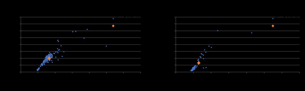
104 Fig. 4.10: Center of daily data (Segment-1 NB). Fig. 4.11: Center of daily data (Segment-2 NB). Fig. 4.12: Center of daily data (Segment-3 NB). 91

105 Fig. 4.7 to 4.12 shows center of daily data for each freeway segment. The daily data shows the data pattern for segment over the year. Detail trend analysis of the data points and qualitative comparison of segment to segment can be done. Table 4.4 shows the vulnerability index of each segment in morning and evening peak period. Table 4.4: Calculation of vulnerability index with daily value. 92

106 Vulneribility Index Buffer Index Prioritization method th percentile travel rate (miles/min) Seg-1 SB AM Seg-3 SB PM Seg-2 SB PM Seg-1 NB PM Seg-2 NB PM Seg-3 NB AM Fig. 4.13: Location of center points to freeway segments (peak direction) in Buffer index vs 95 th percentile travel rate space Vulnerability index in six segments (normal days in peak direction) Seg-1 SB AM Seg-2 SB PM Seg-3 SB PM Seg-1 NB PM Freeway Segments 2.24 Seg-2 NB PM 0.76 Seg-3 NB AM 93

107 Buffer Index Fig. 4.14: Vulnerability index of freeway segment in Peak direction (Prioritization method-2). From fig. 4.13, we can see segment 3 has lower 95 th percentile travel rate and buffer index compared to segment 1. Hence, segment 1 has higher vulnerability index and higher priority compared to segment 3. We analyze the daily data pattern in both segments. From fig. 4.14, it is seen that segment 2 in NB has the highest vulnerability index. Segment 1 in NB has the highest vulnerability index in SB. Segment 2 in SB has the lowest vulnerability index and Segment 3 in SB has the lowest vulnerability index. Buffer index Vs 95th percentile travel rate Seg-1 SB Seg-3 SB th percentile travel rate (miles/min) Fig. 4.15: Buffer index vs 95 th percentile travel rate. From fig. 4.15, it is seen that at the same 95 th percentile travel rate, segment 1 has higher buffer index value (lower travel time reliability) compared to segment 1. In 94

108 segment 3, as congestion goes higher, buffer index value becomes lower. At the high congestion level, the corridor travel time becomes reliable compared to segment-1. The priority of the segments considering the vulnerability index form the prioritization methodology-2 is as follows. Table 4.5: Prioritization of freeway segments (Prioritization method-2). Using the daily data to prioritize freeway segment is beneficial in many ways. Analyzing data pattern can help us to understand the characteristic of a segment. This makes the prioritization of segments more effective. The prioritization method is simple after estimating daily values of travel time and congestion measures. This method can be modified depending on the objective of a project. For example, assigning different weights on different factors can prioritize segments according to the goal of a project. One drawback of the prioritization method is that it does not differentiate between different congestion level and puts all data in a group. As a result, the center point will be closer to the region of the majority data points. This will ignore the effects of the few high congested and highly unreliable days. To overcome these challenges another prioritization method is proposed based on daily data. 95

109 Prioritization Method-3 In this method, the daily buffer index and 95 th percentile travel rate value has also been used. As discussed in chapter 3, buffer index value becomes more scattered when 95 th percentile travel rate is above 1.5. As 95 th percentile travel rate equals 1.5 miles/min, traffic speed gets above 40 mph. Traffic condition is uncongested and in all freeway segment, buffer index range is 0 to 0.4. As speed drops below 40 mph, traffic becomes unstable. Travel time becomes unreliable as the buffer index range becomes wider. To differentiate between high and low congestion levels, the data are divided into two groups as shown in fig st group of data has 95 th percentile travel rate 1.5 or less than 1.5 miles/min. 2 nd group has 95 th percentile travel rate higher than 1.5 mile/min. The 2 nd group is critical data set for a segment as they include highly congested and unreliable days. Center points of the both groups are determined by average buffer index and average 95 th percentile travel rate in that group. Number of data points is also estimated in each group. The distance of center point of group-2 to (1,0) point indicates segment vulnerability because different freeway segments have different number of data points. The percentage of data points in group-2 is multiplied with the distance value to compare segment to segment. Group-1: includes data points with 95 th percentile travel rate is less than or equal to 1.5 miles/min. Group-2: includes data points with 95 th percentile travel rate is greater than 1.5 miles/min. 96

110 Center of daily data points is the average of daily 95 th percentile travel rate and average of daily buffer index in the 95 th percentile travel rate - buffer index space in each group data. d2 is the distance of center of group 2 from (1,0) points. n1is the number of data points in group 1. n2 is the number of data points in group 2. Vulnerability Index is defined as d2*(n2/(n1+n2)). In this method, the data are grouped into two groups. The 1 st group has low congestion and high travel time reliability. The 2 nd group has higher congestion and wider range of buffer index. Low congestion and high reliability in a segment is expected. The 2 nd group indicates the vulnerability state of a given segment. Distance of the center of 2 nd data group from (95 th percentile travel time=1, buffer index=0) is a measure of vulnerability of the segment. Percentage of data points in the 2 nd group indicates how many vulnerable days the segment has in a year. Fig. 4.16: Center point of daily data (Prioritization methodology 3). 97

111 Two groups are formed by using 95 th percentile travel rate. Center of each group is estimated by averaging all the data points in each group. Distance from (1,0) point is determined for each center point. The number of data points are counted in each group to estimate the vulnerability index. Table 4.6: Calculation of vulnerability index with daily value. From fig. 4.13, Segment 2 NB has 94% data points in 2 nd group (95 th percentile travel time greater than 1.5 miles/min and high buffer index range). Segment 1 in NB has 98

112 Buffer Index 85% vulnerable days in evening peak. In SB, all three segments have almost equal percentage of vulnerable days in peak direction. Prioritization method th percentile travel rate (miles/min) Seg-1 SB Seg-3 SB Seg-2 SB Seg-1 NB Seg-2 NB Seg-3 NB Fig. 4.17: Location of freeway segments (peak direction) in Buffer index vs 95 th percentile travel rate plot. From fig. 4.14, segment 2 has the highest buffer index and 95 th percentile travel rate. In NB, segment 3 has higher buffer index than segment 1, but lower 95 th percentile travel rate than segment 1. In SB, segment 1 has the highest buffer index and 95 th percentile travel rate. 99

113 Vulneribility Index Vulnerability index in six segments (normal days in peak direction) Seg-1 SB Seg-2 SB Seg-3 SB Seg-1 NB Seg-2 NB Seg-3 NB Freeway Segments Fig. 4.18: Vulnerability index of freeway segment in Peak direction (Prioritization method-3). From the plot, it is seen that segment 2 in NB has the highest vulnerability index. Segment 1 in NB has the highest vulnerability index in SB. Segment 2 in SB has the lowest vulnerability index and Segment 3 in SB has the lowest vulnerability index. The priority list is following. Table 4.7: Prioritization of freeway segments (Prioritization method-3). This method divides data into two groups and differentiates between high and low congestion levels. It provides additional information about percentage of vulnerable days 100

114 in segment. This method combines the effects of number of vulnerable days and extend of congestion and reliability for prioritization. Table 4.8 shows the comparison of all three prioritization methods. The prioritization method 1 has been applied to normal, weather and incident days. Prioritization method 2 and 3 has been applied to only normal days. Table 4.8: Comparison table for prioritization methods. 4.3 Conclusion Prioritization of freeway segment has significant role in distributing a given budget in improving road geometry and incorporating new facilities. In this chapter, the effects of reliability and congestion are combined to estimate the vulnerability of each segment. This vulnerability index has been used to prioritize freeway corridor. Three 101