SURFACE ENERGY BUDGET OVER INLAND WATER

Transcription

1 SURFACE ENERGY BUDGET OVER INLAND WATER By QIANYU ZHANG A thesis submitted in partial fulfillment of the requirements for the degree of MASTER OF SCIENCE IN ENVIRONMENTAL ENGINEERING WASHINGTON STATE UNIVERSITY Department of Civil and Environmental Engineering MAY 2012

2 To the Faculty of Washington State University: The members of the Committee appointed to examine the thesis of Qianyu Zhang find it satisfactory and recommend that it be accepted. Heping Liu, Ph.D., Chair Brian Lamb, Ph.D. Shelley Pressley, Ph.D. Jennifer Adam, Ph.D. ii

3 Acknowledgements I am grateful to Dan Gaillet, Billy Lester, Jennifer Taylor, Jason Temple, and many other people in Pearl River Valley Water Supply District in Ridgeland, Mississippi, as well as Yu Zhang, Haimei Jiang, Li Sheng, Rongping Li, Yu Wang, and Guo Zhang who contributed to field work. I would like to give special thanks to my advisor, Dr. Heping Liu, for all the science and writing training I received. I would have no chance to finish this thesis if not with his great patience, diligence, and inspiration. I found it was a great fortune to work with him. I would like to thank the committee members, Dr. Brian Lamb, Dr. Shelley Pressley, and Dr. Jennifer Adam, for the advices and opportunities that have strengthened my research experience. Thanks to Dr. Tom Jobson, for his teaching in the useful software technique and advices for surviving in graduate school. I thank all faculty, staff and graduate students at LAR and the Department of Civil and Environmental Engineering for their great supports. I thank many friends who make my stay wonderful at Pullman. Finally, I owe much gratitude to my husband. For his consistent support, I was able to persist and work hard on this thesis. I thank my Dad and Mom very much for their moral and financial support throughout my study at WSU. iii

4 SURFACE ENERGY BUDGET OVER INLAND WATER Abstract By Qianyu Zhang, M.S. Washington State University May 2012 Chair: Heping Liu To better understand water-atmosphere interactions requires direct measurements of the surface energy budget and trace gas exchange over inland waters. In this study, an eddy covariance system was used to measure turbulent fluxes of sensible (H) and latent heat (LE) in 2008 and 2009 over the Ross Barnett Reservoir (hereafter the Reservoir which was ice-free) in Mississippi, U.S.A., to study physical processes that control daily, intra-seasonal, seasonal, and interannual variations in the surface energy budget. Our results indicate that H and LE were distinctively out-of-phase with net radiation (Rn) on different timescales. Fueled by the previously stored heat in the water, the turbulent transfer of H and LE from the water to the atmospheric surface layer (ASL) was still substantial on nights with iv

5 a negative Rn and in winters when Rn was very small. The annual means of net radiation, H, and LE for the two years were 110.6, 15.7, and 83.7 W m 2, respectively. About 81% of the Rn absorbed by the water was transferred to the atmosphere through LE and the remainder was transferred through H. On a monthly basis, the upward, positive temperature and humidity gradients, the unstable ASL, and the sufficient mechanical mixing were observed, leading to persistent positive H and LE. Intraseasonal and seasonal variations in turbulent exchanges of H and LE were strongly affected by alternative incursions of large-scale air masses brought in by different synoptic weather systems (e.g., cyclones or anticyclones) throughout the two years. Southerly winds with tropical maritime air masses (warm and humid) from the Gulf of Mexico and northerly winds with continental air masses (cool and dry) produced two distinctive atmospheric forcings for the water-air interactions. Interannual variability in the surface energy budget was modulated by variations in mean climate conditions as well as by differences in these synoptic weather events. It suggests that possible shifts in northerly and southerly winds associated with changes in synoptic weather events would have significant impacts on seasonal, annual, and interannual variations in the water surface energy budget, evaporation rates, and hydrologic processes in this region. v

6 Table of Contents Acknowledgements... iii Abstract... iv Table of Contents... vi List of Figures... ix List of Tables... xi Symbols... xii 1. Introduction Methods Site description The surface energy balance over water Instruments Postfield processing of eddy covariance data Results and discussion General climate Temperature and precipitation Synoptic weather patterns General characteristics of the surface energy budget in 2008 and vi

7 3.3 Seasonal variations General seasonal variations in the surface energy budget Factors controlling seasonal variations in H Factors controlling seasonal variations in LE Diurnal variations General diurnal variations in the surface energy budget Diurnal variations and controlling factors in winter (JFM) Diurnal variations and controlling factors in summer (JJA) H and LE pulses and their contributions to interannual variations in H and LE Definition of H and LE pulses Physical processes to generate H and LE pulses Contributions of H and LE pulses to the surface energy budget Interannual variations Factors modulating interannual variations in H and LE General statistical analysis of winds for 2008 and Mechanisms controlling turbulent exchanges Comparison of the surface energy budget with high-latitude northern lakes Comparison of the annual mean surface energy budget and cumulative evaporation vii

8 3.8.2 Comparison of seasonal variations in the surface energy budget Summary and conclusions References viii

9 List of Figures Figure 1. Location of the study site in Ross Barnett Reservoir, Ridgeland, Mississippi... 8 Figure 2. Schematic view of the water surface energy balance... 9 Figure 3. Annual mean temperature and precipitation from 1964 to Figure 4. Monthly mean temperature and precipitation at the Jackson International Airport Figure 5. Half-hourly means of the energy fluxes in 2008 and Figure 6. Half-hourly means of meteorological variables in 2008 and Figure 7. Daily means of the components of the surface energy budget for 2008 and Figure 8. Two-year averaged half-monthly means of the surface energy budget Figure 9. Two-year averaged half-monthly means of atmospheric and limnological variables Figure 10. Two-year averaged monthly diurnal cycles of Rn, H, and LE Figure 11. Two-year averaged monthly diurnal cycles of water surface temperatures Figure 12. Diurnal variations of energy fluxes and meteorological variables in winter Figure 13. Linear regressions of the diurnal LE and diurnal H Figure 14. Diurnal variations of energy fluxes and meteorological variables in summer Figure 15. Linear regressions of the diurnal H against UΔT, ΔT, U, and z/l in summer Figure 16. Linear regressions and temporal sequences of LE in summer Figure 17. H pulses in 2008 and ix

10 Figure 18. LE pulses in 2008 and Figure 19. Daily weather maps showing the passage of a cold front in February of Figure 20. Comparisons of winds within and outside a H and LE pulse Figure 21. Changes in surface energy fluxes and meteorological variables after a cold front Figure 22. Wind rose diagrams for 2008 and Figure 23. Relationships of half-hourly H and of half-hourly LE Figure 24. Scatter plots of U against Δe on the diurnal timescale in the winter and summer Figure 25. The linear relationship between LE and Δe, or U in winter Figure 26. The linear relationship between LE and Δe, or U in summer Figure 27. Relationships of LE, U, and Δe for different Δe ranges in winter and summer Figure 28. Comparison of annual radiation cycles for lakes in low- and high-latitues Figure 29. Comparison of the annual LE, H, and z/l for lakes in low- and high-latitues x

11 List of Tables Table 1. List of the instruments used in this study Table 2. Summary of 30-min data and their quality in 2008 and Table 3. Monthly mean temperature and precipitation at the Jackson International Airport Table 4. Half-monthly averaged meteorological variables and surface energy budget Table 5. Correlation coefficients between LE (H) and external forcings Table 6. Comparisons of energy fluxes and meteorological variables of a pulse event Table 7. Two-year averaged daily mean H and LE for pulse and non-pulse days Table 8. Interannual variations of the energy fluxes and meteorological variables Table 9. Percentage of winds from the north, south, east, and west in 2008 and Table 10. Comparison of the annual mean LE and cume for lakes in low- and high-latitues xi

12 Symbols α ASL B C E C H C p C pw Ctrn.Flux(PS)% cume Days(PS) e a e w Δe EBC EBEX Flux(PS) G GSL H IRGA JFM JJA K p K K L L L LE LT Albedo Atmospheric surface layer Bowen ratio, calculated as sensible heat flux divided by latent heat flux Bulk transfer coefficients for moisture Bulk transfer coefficients for heat Specific heat of air Specific heat of water Contribution of the flux in percentage to the overall flux Cumulative evaporation Pulse days with H and LE pulses Atmospheric vapor pressure Saturation vapor pressure at the water surface layer temperature, T w Δe = e w e a, vertical gradient of vapor pressure over the water surface Energy balance closure Energy balance experiment Averaged daily mean of the flux during the pulse days Heat flux into the water Great Slave Lake Sensible heat flux Open path CO 2 /H 2 O infrared gas analyzer January, February, and March June, July, and August Penetrating solar radiation through water surface into deeper layers Incident shortwave radiation Reflected shortwave radiation Latent heat of vaporization Incoming longwave radiation Outgoing longwave radiation Latent heat flux Local time xii

13 ρ c ρ v ρ w P Q A Q B Carbon dioxide density Water vapor density Water density Mean precipitation Net horizontal heat flux into or out of the water column Heat flux through the bottom sediments of the Reservoir q Specific humidity fluctuation RBR REBS Res RH Rn R 2 So τ T T s T 0 T a T w ΔT T wi Ross Barnett Reservoir Radiation and Energy Balance Systems Surface energy budget residual, calculated as the residual of Rn H LE Relative humidity Net radiation Linear correlation coefficient Incoming solar radiation Reynolds stress Annual mean temperature Sonic temperature Water surface skin temperature Atmospheric temperature Water surface layer temperature ΔT = T w T a, vertical gradient of temperature over the water surface The i th water temperature profile measurements T wi Mean water temperature change at the i th layer over the period Δt ΔQ s Change in heat storage within the water column u, v, w Turbulent fluctuations of wind velocity components U WD Wind speed Wind direction µ Molar mass ratio of dry air to water vapor u * Friction velocity (m s 1 ) z wi z/l σ Water depth for the i th layer Stability parameter, z: the measurement height, L: Monin-Obukhov length Ratio of mean water vapor density to dry air density xiii

14 1. Introduction Inland fresh waters (e.g., lakes, reservoirs, wetlands, etc) compose a large portion of the land surface [Bonan, 1995]. These water bodies have unique characteristics in albedo, heat capacity, and roughness; and they behave differently from surrounding lands in terms of exchanges of radiation, energy, water vapor, and trace gases between the surface and the overlying atmosphere [Bonan, 1995; Eaton et al., 2001; MacIntyre et al., 2006; Magnuson et al., 2000; Walter et al., 2006]. Previous studies suggest that inland water bodies can exert significant influences on climate in regions where they are abundant and important [Bates et al., 1995; Blanken et al., 2003; Bonan, 1995; Cole et al., 2007; Eaton et al., 2001; Long et al., 2007; Rouse et al., 2005]. For example, based on measurements, it was estimated that including water bodies in the central Mackenzie River basin of western Canada region substantially increased regional net radiation (Rn), the maximum regional subsurface heat storage, and latent heat fluxes (LE), but substantially decreased sensible heat fluxes (H) [Rouse et al., 2005]. It was also reported that the presence of the Great Lakes in general circulation model (GCM) cases resulted in a phase shift in the annual cycle of LE and H, as opposed to land [Lofgren, 1997]. It is projected that global hydrologic cycles will be intensified as a result of global warming and, in turn, they promote warming via the positive water vapor-temperature feedback [Huntington, 1

15 2006; Solomon et al., 2007]. The surface energy budget over open inland waters should be used as a protocol in detecting climate change, since it is not complicated by adaptive physiological responses of terrestrial vegetation [Blanken et al., 2000]. The integrated response of large inland waters to climate variability and seasonal perturbations through the large surface area and volume of water would provide a robust indicator as to whether global warming has the potential to accelerate the energy and water vapor (and thus evaporation) exchange between inland waters and the atmosphere. Thus direct measurements of the surface energy budget over inland waters are required so as to better understand the impacts of climate change or climate variability on the evaporation and hydrologic cycles [Blanken et al., 2000; Oswald and Rouse, 2004]. Implications of changes in the surface energy budget in response to climate change are also of major significance for the local water resource management through the process of evaporation since evaporation is proportional to LE. In addition, the improvement of regional climate models for regions with inland water bodies requires details in the water surface-atmosphere interaction mechanism. In situ observations made at large inland waters would provide robust verification tools for regional climate models [Long et al., 2007]. The large inland water responds to atmospheric forcings significantly differently from the surrounding lands [Bonan, 1995; Eaton et al., 2001]. At the water surface, shortwave radiation that is not reflected back to the atmosphere may penetrate to deeper layers and is directly 2

16 absorbed by the water. The amount of solar radiation absorbed by water exponentially decreases with depth and is dependent on water turbidity, which is influenced by suspended organic and inorganic materials [Hendersonsellers, 1986; Hostetler and Bartlein, 1990]. In addition to heat transfer by conduction, water eddy diffusion leads to efficient heat transfer under the water surface [Hendersonsellers, 1986]. In contrast, the land surface absorbs and emits radiation fast due to its small heat capacity, and heat transfer in soils only relies on heat conduction for energy transfer, which is much less efficient. As a consequence, although water surfaces have slightly lower albedo than land surfaces ( for water and for lands) [Budyko, 1974], they exhibit different responses to the diurnal and seasonal changes in the solar radiation forcing, leading to distinct temporal variations in the surface temperature. It is well known that H is primarily determined by the temperature difference between the water surface and the overlying atmosphere as well as the turbulent exchange coefficient, while LE is dependent upon vapor pressure differences at the water-air interface as well as upon the turbulent mixing intensity [Bonan, 1995; Garratt, 1992; Hendersonsellers, 1986; Hostetler and Bartlein, 1990; Nordbo et al., 2011]. The water surface is almost always at its saturation point, and vapor pressure at the surface is a function of the water surface temperature [Hostetler and Bartlein, 1990], making the water surface temperature a key element in determining the water-atmosphere energy exchange. Consequently, temporal variations in H and LE are largely governed by 3

17 variations in the water surface temperature and the meteorological properties (e.g., wind speeds, air temperature and humidity) of over-water air masses [Rouse et al., 2008; Schertzer et al., 2003]. Studies of large high-latitude lakes indicate that the water stores a large amount of solar energy in the spring and summer, leading to a gradual increase in water temperature [Rouse et al., 2003; Winter et al., 2003]. Since the water temperature increases much more slowly than the overlying air, there is a thermal inversion, or small temperature difference, between the water surface and the overlying atmosphere. During this heating stage, H and LE are usually dampened due to the presence of the stably stratified atmospheric surface layer (ASL) [Oswald and Rouse, 2004]. As the seasons progress into the fall and winter when the absorbed solar radiation is small the air temperature decreases at a faster rate and becomes lower than the water temperature, leading to a large positive temperature gradient and an unstable ASL. It is expected that evaporation usually occurs during this period, since continental air masses in the ASL are almost always drier than the water-air interface, where water vapor pressure is nearly at saturation, producing positive vapor pressure gradients in the ASL [Blanken et al., 2003; Lenters et al., 2005]. In some cases, however, condensation may occur when warm and humid air masses pass over water which is cold enough to make the vapor pressure of the air masses greater than the saturation pressure in the water-air interface [Blanken et al., 2000; Liu et al., 2009]. 4

18 As long as mechanical turbulence mixing is sufficient, H and LE (and thus evaporation) are promoted when the ASL is unstable, and depressed when the ASL is stable. In the wintertime, when net radiation (Rn) is small, H and LE are still substantial. This energetic exchange of sensible and latent heat between the water surface and the atmosphere is fueled by the energy previously stored in the water, acting as an energy source [Rouse et al., 2005]. It remains unclear whether these observed physical processes that govern energy and moisture exchanges between large northern high-latitude lakes and the atmosphere are applicable to mid- and low-latitude inland waters [Sacks et al., 1994; Vallet-Coulomb et al., 2001]. Previous efforts have also focused on studying the significant intraseasonal variations that are strongly associated with synoptic weather events and strong wind activities [Blanken et al., 2003; Blanken et al., 2000; Lenters et al., 2005; Liu et al., 2009; Rouse et al., 2003]. For instance, it was found in the Great Slave Lake that for its ice-free season, more than 50% of the measured evaporation occurred over only 25% and 20% of the days for the studied two years, in association with the passages of cold, dry air masses over the lake. These passages of cold, dry air masses led to large H and LE events which contributed to substantial increases in evaporation in high-latitude lakes (e.g., [Blanken et al., 2003; Lenters et al., 2005]). These large H and LE events (pulses) were also present over a large southern reservoir, occurring during 26% of the 5

19 days in the cool season and increasing the seasonal H by 42% and LE by 157%, respectively [Liu et al., 2009]. These large H and LE events were also associated with cold front activities in this region [Liu et al., 2009], and contributed to differences in the surface energy budget between two cool seasons due to changes in frequency, duration, and intensity of the events [Liu et al., 2011]. It has not been studied yet as to whether different synoptic weather activities between two years affect interannual variations in the water surface energy budget and evaporation rates. Although these previous studies provide useful analyses on the water-atmosphere interactions, particularly in high latitudes, there is still a lack of direct, long-term measurements of the water surface budget over mid- to low-latitude regions. In this study, we report eddy covariance measurements and analyses of the surface energy budget over the Ross Barnett Reservoir, a large inland water in central Mississippi, over the course of 2008 and This study will contribute to knowledge gained from others that use the eddy covariance technique for longer-term measurements of the surface energy budget over water in high-latitudes [Blanken et al., 2008; Blanken et al., 2000; Nordbo et al., 2011; Vesala et al., 2006]. The objectives of this study are to quantify seasonal, diurnal, and interannual variations in the surface energy budget and analyze the mechanisms that control H and LE on these timescales. 6

20 2. Methods 2.1 Site description Ross Barnett Reservoir is located in central Mississippi (32 26'N, 90 02'W), serving as the state s largest drinking water resource (Figure 1). It is fed by the Pearl River from the northeast, and discharges into a river in the south through a 3.5-mile man-made dam and spillway. On average, the reservoir has a surface area of about 33,000 acres (130 km 2 ) and the water depth varies from 4 to 8 m. The water elevation is 90.7 m above sea level in summer and 90.2 m in winter. A stationary wood platform was constructed and located in the south center of Ross Barnett Reservoir. It had a deck area of 3 m 3 m and was approximately 1.6 m above the water surface when it was initially built in August of The water around the platform was 5 m in depth on average. A 5 m tower (Climatronics Corp.) was installed and mounted over the platform (Figure 1). The distance from the tower to shore ranged from 2.0 km to more than 10 km to minimize the footprint influences on fluxes from the surrounding lands (Figure 1). 7

21 Ross Barnett Reservoir (32 26' N, 90 02' W) 2km Figure 1. Location of the study site in Ross Barnett Reservoir, Ridgeland, Mississippi (Google 2012). Triangle in the bottom left panel denotes the tower location ( N, W) 8

22 2.2 The surface energy balance over water The surface energy budget for the water surface may be represented through Eq. (1) and its schematic view is shown in Figure 2. Rn H LE G K = 0 (1) where Rn denotes the net radiation measured at the water surface (positive for absorption by the surface); K p is the solar radiation that penetrates through the water surface into the deeper layers; H is the positive sensible heat flux out of the surface; LE is the positive latent heat flux out of the surface; G represents the downward heat flux which is transferred by both molecular conduction and large eddy diffusion from the water surface to the deeper layers (all energy terms expressed in W m 2 ). p Sun LE K K = α K L L H Water surface K p G Figure 2. Schematic view of the water surface energy balance. K : incident shortwave radiation, K : reflected shortwave radiation, α: albedo, Kp: penetrating shortwave radiation, L : incoming longwave radiation; L : outgoing longwave radiation, H: sensible heat flux, LE: latent heat flux, G: water heat flux. 9

23 Specifically, the net radiation absorbed by the water surface (Rn K P ) is the net result of incoming solar radiation (K ), reflected solar radiation (K ), incoming long-wave radiation (L ) and outgoing long-wave radiation (L ), and, as described by Rn K p = K K + L L (2) For the water column below the water surface down to the water-sediment interface, the energy balance can be described by K p + G = Q + Q + Q (3) B A S where Q B is the heat flux through the bottom sediments of the Reservoir, Q A is the net horizontal heat flux brought by horizontal water currents into or out of the water column, ΔQ S is the change in heat storage within the water column (positive for warming) and can be quantified by change in water temperatures, as Q S ρwc = n pw i=1 t T wi z wi (4) where ρ w is the density of water (kg m 3 ), C pw is the specific heat of water (J C kg 1 ), z wi is water depth (m) for i th layer where the i th water temperature profile measurements (T wi ; C) were made (n = 8 in this study). Therefore, Twi is the mean water temperature change at the i th layer over the period Δt. Previous studies indicated that Q B can be neglected because it only contributes less than 5% of 10

24 the heat storage change in lakes [Stannard and Rosenberry, 1991; Sturrock et al., 1992]. Q A is negligible for water bodies with small inflow and outflow volumes, which is particularly true for this reservoir. It was found that large errors can be induced in determining ΔQ S (based on Eq. (4)) due to localized changes in water temperatures by water eddy diffusion, thus the energy budget residual (Res) is widely applied to obtain ΔQ S, based on Equations (1), (2) and (3) [Blanken et al., 2003; Lenters et al., 2005; Nordbo et al., 2011]. = Re s = Rn H LE (5) Q S This study will used Eq. (5) to estimate ΔQ S in particular because of the lack of high quality surface water temperatures (as explained in more detail later). 2.3 Instruments In this study, an eddy covariance system was mounted 4 m above the water surface, including a three-dimensional sonic anemometer (model CSAT3, Campbell Scientific, Inc.) and an open path CO 2 /H 2 O infrared gas analyzer (IRGA; Model LI-7500, LI-COR, Inc.). The sonic anemometer measured turbulent fluctuations of wind velocity components (u, v, and w) and fluctuations of sonic temperature (T s ). The IRGA measured fluctuations of densities of carbon dioxide (ρ c ) and water vapor (ρ v ). The horizontal distance between the sonic anemometer and the IRGA was approximately 20 cm. Signals from the eddy covariance sensors were recorded at a frequency of 11

25 10 Hz by a datalogger (model CR5000, Campbell Scientific, Inc.). The turbulent fluxes of sensible heat, latent heat and momentum in kinematic forms can be quantified as the 30-min mean covariance between w and c, where c is respective quantity as ~ H = w' T S ' (6) LE = w' ρv ' (7) ~ τ w (8) 2 2 Re ynolds = ρ ( u a w ) + ( v ) For each variable the prime in the above equations represents instantaneous departures from its 30-min mean. We also measured a variety of meteorological variables as 30-min averages of 1 s readings. Net radiation (Rn) was measured using a net radiometer (model Q-7.1, Radiation and Energy Balance Systems (REBS), Campbell Scientific, Inc.). It was mounted approximately 1.2 m above the water surface. Incoming solar radiation was measured with a silicon pyranometer (model LI-200, LI-COR, Inc.). Air temperature (T a ) and relative humidity (RH) were measured using temperature and humidity probes with 10-plate radiation shields (model HMP45C, Vaisala, Inc.) on the tower at approximately 1.9, 3.0, 4.0, and 5.46 m above the water surface. Wind speeds (U) and wind direction (WD) were measured using a wind sentry unit (model 03001, RM Young, Inc.) at 5.46 m. Three other wind speed sensors (model 03101, RM Young, Inc.) were mounted at heights of 1.9, 3.0, and 4.0 m above the water surface with the HMP45C humidity probes. 12

26 Water surface temperature (T 0 ) was measured using an infrared temperature sensor (model IRR-P, Apogee, Inc.). T 0 was not used in this study due to the malfunction of the infrared temperature sensor since the beginning of The water temperature profile was measured by temperature sensors (model 107-L, Campbell Scientific, Inc.) which were attached to a buoy and placed at depths of 0.10, 0.25, 0.5, 1.0, 1.5, 2.5, 3.5, and 4.5 m below the water surface. The water temperature measured at 0.5 m depth was used to represent the water surface layer temperature (T w ) for this study. Vapor pressure (e w ) at the water surface was estimated by calculating the saturation vapor pressure at the water surface layer temperature (T w ). Precipitation was measured using a tipping bucket rain gauge to obtain 30-min accumulative precipitation rates (model TE525, Texas Instruments, Inc.). Table 1 lists all of the instruments used in this study and their corresponding measurement heights. Two solar panels (model SP65, 65 Watt Solar Panel, Campbell Scientific, Inc.) were mounted on the platform to charge six deep cycling marine batteries and provide power for all the instruments. All slow-response sensor signals were also recorded with the CR5000 datalogger at 30-min intervals. The 30-min average data were accessed from shore through a wireless radio system (model FGR-115RC, FreeWave 900 MHz Spread Spectrum Radio, 1 Watt, FreeWave Technology, Inc.). The instruments were checked and maintained and the 30-min time-series data were downloaded on a monthly basis. 13

27 Table 1. List of the instruments for fast-response (10 Hz) and for slow-response (1 s) used in this study. Instruments Variables Model and maker Heights/Depths (m) Fast-response variables measured at 10 Hz Three-dimensional sonic anemometer u, v, w, T s model CSAT3, Campbell Scientific, Inc. 4.0 Open path CO 2 /H 2 O infrared gas analyzer ρ v, ρ c model LI-7500, LI-COR, Inc. 4.0 Slow-response variables measured at 1 s Net radiometer Net radiation (Rn) model Q-7.1, Campbell Scientific, Inc. 1.2 Silicon pyranometer Incoming solar radiation model LI-200, LI-COR 1.2 (So) Inc. Temperature and Air temperature (T a ) model HMP45C, 1.9, 3.0, 4.0, and 5.46 humidity probe Relative humidity (RH) Vaisala, Inc. Wind sentry unit Wind speed (U) and model 03001, 5.46 wind direction (WD) RM Young, Inc. Wind speed sensor Wind speed (U i ) model 03101, RM Young, Inc. 1.9, 3.0, and 4.0 Infrared temperature Water surface temperature model IRR-P, - sensor (T 0 ) Apogee, Inc. Temperature sensor Water temperature (T w ) model 107-L, Campbell Scientific, Inc. 0.10, 0.25, 0.5, 1.0, 1.5, 2.5, 3.5, and 4.5 Tipping bucket Precipitation model TE525, - rain gauge Texas Instruments, Inc. 14

28 A summary of the 30-min data and their availability is listed in Table 2. Considering all missing and rejected data, data availability was good in 2008, with around 95% available data points for each measured variable. In 2009, S o (incoming solar radiation), Rn, T a, T w and RH were of good quality with around 93% available data points, while the percentage for available H, LE, and wind speed data points were only 80%, 80%, and 87%. Note that data gaps were caused by instrument failures, calibrations, and precipitation, especially for H and LE. Table 2. Summary of 30-min data and their availability in 2008 and Data gaps were caused by instrument failures, calibrations, and precipitation. Variable Unit Year Mean Max Min Stdev Data points (%) So W m Rn W m H W m LE W m T a ºC T w ºC U m s RH % Major data gaps month (days) 2008 Feb (4) and Dec (11) 2009 Jan (4), Mar (5), May (13), Jun (5), Aug (4), Sep (11), Oct (17) and Dec (12) 15

29 2.4 Postfield processing of eddy covariance data Raw time-series turbulence data collected in this study were processed and corrected to obtain eddy covariance fluxes, using a postfield data processing program [Liu et al., 2005]. This program was used in the energy balance experiment (EBEX) [Mauder et al., 2006], and has been updated following recommendations by Mauder and Foken [2004] since then [Liu et al., 2009]. The following data processing steps were performed. [Mauder and Foken, 2004] 1. Despiking: Data spikes in eddy covariance systems may be caused by random electronic spikes in the instruments or by precipitation collecting on sonic transducers or the window of gas analyzers [Vickers and Mahrt, 1997]. The despiking routine developed by Hojstrup [1993] has been widely used in the flux community and therefore was followed in this study [e.g., Foken et al., 2012]. To apply this method, the mean and standard deviation for a series of moving windows with a certain window length was first computed. The window moved forward one value at a time. Any value exceeding several times its standard deviations was considered a spike, unless four or more consecutive points were detected, in which case the spike was considered to be physical. Spikes were then replaced by linear interpolation. We took the window length to be 10 (corresponding to 1 second), as in Hojstrup [1993] and Mauder and Foken [2004]. We used a value of 5.5 times the standard deviations in our calculation, as suggested by Vickers and 16

30 Mahrt [1997]. [Foken et al., 2012] [Hojstrup, 1993] [Hojstrup, 1993; Mauder and Foken, 2004] [Vickers and Mahrt, 1997] 2. Coordinate Rotation: We used the double rotation for rotating the coordinate system for each averaging period (i.e., 30 minutes in this study). First the x-y plane was rotated at angle α about the z-axis such that: v α = tan 1 ( ) (9) u The new x-z plane was then rotated at angle β such that: 1 w β = tan ( ) (10) 2 2 u + v After the two rotations, we obtained v = w = Block Averaging: We used 30 minute block averaging to obtain the means for time-series data, which were then removed from the raw data to get the fluctuating quantities for further calculations. Note that the calculated mean fluxes are affected by the choice of averaging period. Short averaging periods lead to a loss of the low frequency contributions to the fluxes, while long averaging periods the steady state condition may not be fulfilled. The 30 min block averaging is recommended to use over the whole day [Foken, 2008]. However, it has been shown that the 30 min block averaging underestimates the fluxes by 4-17% [Finnigan et al., 2003; Sakai et al., 2001]. 17

31 4. Flux Calculations: Preliminary sensible, latent and momentum fluxes in kinematic form were first calculated using Eqs. (6), (7), and (8), respectively. Since we did not use a fine wire thermocouple in the eddy covariance system for temperature measurements, the sonic temperature was used for calculating sensible heat flux (Eq. (6)). Because the speed of sound is dependent on humidity in addition to temperature, heat flux from Eq. (6) must be corrected for the effect of moisture fluxes. This correction is discussed in detail in step Webb Pearman and Leuning (WPL) Corrections: Due to the density effects, latent heat fluxes obtained by Eq. (7) must be corrected according to WPL corrections [Webb et al., 1980]. When the temperature and humidity fluctuations are known, the latent heat flux after WPL corrections can be obtained as ρ v w ρ = + w + w T vc (1 µσ ) ρv ( ) (11) T where µ is the molar mass ratio of dry air to water vapor, and σ is the ratio of mean water vapor density to dry air density. 6. Sonic Temperature Correction: Sonic anemometers derive temperature measurements from the speed of sound in air, which is affected by crosswind and changes in humidity [Liu et al., 2001; 18

32 Schotanus et al., 1983]. However, crosswind corrections were made internally in the CSAT3 sonic anemometer (Campbell Scientific Inc.). Therefore, sensible heat fluxes obtained by Eq. (6) must be corrected for humidity fluctuations by: w T sc = w T s T w q (12) where q is the specific humidity fluctuation and T is the average air temperature which was measured by a HMP45C in this study. 7. Convergence Test: It can be seen in steps 4, 5, and 6 that the sensible and latent heat fluxes were interdependent. Therefore, steps 4-6 were typically iterated until the difference in fluxes between iterations was 0.01% or less [Mauder and Foken, 2004], yielding sensible (H) and latent (LE) heat fluxes reported in this study; H = ρ C w T (13) a p vc sc LE = L w ρ (14) where ρ a is the air density, C p is the specific heat of air, and L is the latent heat of vaporization. Additionally, friction velocity (u * ) reported in this study was defined by the relation 2 τ Re ynolds = where τ is the Reynolds stress and ρ a is the air density. u (15) ρ a 19

33 3. Results and discussion 3.1 General climate Temperature and precipitation Mississippi is located in the subtropical zone, with short mild winters and long, hot and humid summers. The data from a climate monitoring station at the Jackson International Airport, 15 km southeast of the study site, indicate that the 47-year mean air temperature and precipitation from 1964 to 2010 were 18.2 C and 1,398 mm, respectively (Figure 3; National Climatic Data Center, The temperature records show that the Jackson area has been warming at a rate of 0.13 C per dec ade during the past 47 years. No statistically significant trend was found for the precipitation. Figure 3. Annual mean temperature (T) and precipitation (P) from 1964 to 2010 at the Jackson International Airport, Mississippi. Figure on the left shows the 0.13 C per decade warming trend for this area during the last 47 years. 20

34 Both the annual mean air temperatures for 2008 and 2009 were 18.3 C and slightly above the 47-year mean of 18.2 C. There was slightly more precipitation in 2008 (1,514 mm) than in 2009 (1,442 mm). Monthly mean temperatures showed similar patterns in 2008 and 2009 (Figure 4, Table 3). Temperatures increased from 7.3 C (8.6 C) in January to 28.3 C in July (27.6 C in June), and decreased to 10.1 C (7.6 C) in December for 2008 (2009). Precipitation showed no particular patterns and was unevenly distributed throughout the years. Figure 4. Monthly mean temperature (T) and precipitation (P) at the Jackson International Airport Table 3. Monthly mean temperature (T) and precipitation (P) at the Jackson International Airport Month Jan Feb Mar Apr May Jun Jul Aug Sep Oct Nov Dec Average T ( C) P (mm) T ( C) P (mm)

35 3.1.2 Synoptic weather patterns Throughout a year, this region is under the alternate influences of anti-cyclonic and cyclonic weather systems, bringing in air masses originating from different sources [Liu et al., 2009]. In the warm season (defined in this study as months from April to September), the Bermuda high circulates warm, humid air northward from the Gulf of Mexico into the southeast. In the cool season (defined in this study as months from October to March), the Canadian high dominates over North America, bringing north and northwestern cold, dry air masses into the south, accompanied by occasional cold front events [Ahrens, 2011]. We hypothesize that 1) seasonal shifts in synoptic weather patterns, which lead to changes in meteorological conditions of air masses, significantly govern seasonal variations in the water surface energy budget and evaporation; and 2) year-to-year variations in synoptic weather events are partly responsible for interannual variations in the water surface energy budget and evaporation. 22

36 3.2 General characteristics of the surface energy budget in 2008 and 2009 The half-hourly time series data and daily means of Rn, H, LE, and the energy budget residual (Res = Rn H LE) are shown in Figures 5, 6, and 7. Rn exhibited clear diurnal cycles with positive values in the daytime and negative ones at night (Figure 5). Over the two years, the daytime maximum 30-min Rn ranged from about 400 W m 2 in January to about 800 W m 2 in July, and the nighttime 30-min Rn ranged from about 150 to 50 W m 2, resulting in daily means from 50 to 250 W m 2 (Figures 5, 7). Positive 30-min Rn occurred occasionally at nights due to warm air mass movements over this region, leading to a temperature inversion above the water surface and thus larger incoming longwave radiation than outgoing longwave radiation. H and LE also had clear intraseasonal variations in response to short-term variations in meteorological forcings (e.g., temperature, humidity, wind speeds, etc.) (Figure 5). H was relatively small in the warm season and large in the cool season, while LE was large in the warm season and relatively small in the cool season. On a few occasions, daily mean H reached a maximum of 150 W m 2 or a minimum of 50 W m 2 (Figure 7). By contrast, LE ranged in its daily means from about 100 W m 2 to 400 W m 2 in the cool season and from 50 W m 2 to more than 500 W m 2 in the warm season. Negative LE seldom occurred in the warm season and occasionally in the cool season due to the moist air masses passing over the water surface. 23

37 24 Figure 5. Half-hourly means of the energy fluxes in 2008 and 2009; Rn: net radiation, H: sensible heat fluxes, LE: latent heat fluxes, and Res: energy budget residual (Res = Rn H LE). Data gaps were caused by instrument failures, calibrations, and precipitation.

38 25 Figure 6. Half-hourly means of meteorological variables in 2008 and 2009; U: wind speeds, T a : air temperature, T w : water temperature, and e a : vapor pressure. Data gaps were caused by instrument failures, calibrations, and precipitation.

39 Figure 7. Daily means of the components of the surface energy budget for 2008 and Data gaps were caused by instrument failures, calibrations, and precipitation. The energy balance closure (EBC, %) was analyzed based on the available data in 2008 followed the method of Nordbo et al. (2011). The monthly EBC varied between 85% and 117% and the annual mean was 97%. The EBC were greater than 100% (i.e., ranging from 103% to 117%) from February to June and less than 100% for the rest of the months. Particularly, the lowest EBC values occurred in November (88%), December (85%), and January (87%). 26

40 It is noted that the diurnal and even intraseasonal variations of H and LE were characterized by occasionally large H and LE pulses that were evident throughout the two years (Figures 5, 7). These H and LE pulses are distinguished by large, positive H and LE magnitudes that persisted for up to a few days. Additionally, the signatures of the diurnal variations in H and LE were diluted and superimposed with these H and LE pulses. In general, H and LE pulses occurred more often in the cool season than in the warm season. It is apparent that H (LE) pulses had larger (smaller) magnitudes in the cool season than the warm season. Further analysis indicated that these H and LE pulses were associated with high-wind events that corresponded to large wind speeds (U) as the direct consequence of a synoptic weather event. Previous studies at this site for a cool season indicated that these high-wind events (i.e., U spikes in Figure 6) were usually associated with cold, dry air masses immediately behind cold fronts, which created large vertical gradients of temperature and vapor pressure (i.e., large T w T a and e w e a in Figure 6) in the ASL [Liu et al., 2009]. Strong mechanical mixing and the enhanced convective atmospheric surface layer (ASL) promoted turbulent exchanges of sensible and latent heat, generating episodic H and LE pulses [Blanken et al., 2000; Lenters et al., 2005; Liu et al., 2009]. We hypothesize that these strong intraseasonal variations in H and LE pulses significantly contributed to the seasonal variations in the surface energy budget and also contributed to the interannual variations in the surface energy budget. 27

41 Given the substantial variability in the surface energy budget on each of these three timescales, we focused our analyses on the (1) seasonal, (2) diurnal, (3) interannual variations of the surface energy budget, as well as the impacts of H and LE pulses on the surface energy budget. The controlling factors for the surface energy budget on each timescale were also examined. The objectives for such analyses were to investigate physical processes and mechanisms that regulate diurnal, seasonal, and interannual variations in the surface energy budget over a southern inland water surface. We then compared our results with studies over other regions, aiming to examine applicability of our conclusions obtained over this low-latitude inland water in other geographical locations. 3.3 Seasonal variations General seasonal variations in the surface energy budget The general features of Rn, H, and LE on the seasonal scale can be analyzed through their half-monthly means over the course of the years (Figure 8a, Table 4). On the half-monthly basis, Rn presented a clear pattern associated with solar radiation. It increased gradually from 33.4 W m 2 in January, reached its maximum of W m 2 in June, and then leveled off afterwards to its minimum of 15.2 W m 2 in December. Rn remained positive throughout the year, continuously providing the primary energy input for heating water. 28

42 Figure 8. Two-year averaged half-monthly means of the surface energy budget: a) net radiation (Rn) and sensible (H) and latent (LE) heat fluxes, b) Bowen ratio (B), and c) the energy budget residual (Res = Rn H LE). Only data in the second half of May are available for The data in the second half of December for both years are not included due to large gaps in data points. 29

43 30 Table 4. Half-monthly averaged components of the surface energy budget and meteorological variables in 2008 and Table parameters are defined in the notes at the bottom of the table. Month Half So Rn H LE Res B u * U RH T a T w ΔT e a e w Δe W m 2 W m 2 W m 2 W m 2 W m 2 m s 1 m s 1 C C C kpa kpa kpa Jan 1st nd Feb 1st nd Mar 1st nd Apr 1st nd May* 1st nd Jun 1st nd Jul 1st nd Aug 1st nd Sep 1st nd Oct 1st nd Nov 1st nd Dec 1st nd Mean Notes: So: incoming solar radiation, Rn: net radiation, H: sensible heat flux, LE: latent heat flux, Res: the energy budget residual (Res = Rn H LE), B: Bowen ratio, u * : friction velocity, U: wind speed, RH: relative humidity, T a : air temperature, T w : water temperature at 0.5 m depth, ΔT: vertical temperature gradient between the water surface and the air, e a : vapor pressure in the atmosphere (T w T a ), e w : vapor pressure at the water-air interface calculated using T w, Δe: vertical vapor pressure gradient between water surface and the air (e w e a ).

44 H showed no correspondence to the pattern of Rn (Figure 8a). In the warm season, the half-monthly average H was relatively small and varied little, increasing gradually from the low value of 6 W m 2 in late April to the high value of 20.6 W m 2 in late August as the seasons progressed (Table 4). In the cool season, H became larger and had more variances, ranging between 4.4 W m 2 in late February to 28.5 W m 2 in late October. The largest H fluctuation occurred in February, when H decreased by 80% during the first half of February, and increased by a factor of 3.7 during the second half. Compared with the large values of Rn and LE, the generally small H indicates that only a small amount of Rn absorbed by the water was used for the sensible heating of the atmosphere. Different from H, LE followed the seasonal variation patterns of Rn quite well. The half-monthly average LE increased from about 50 W m 2 in January, reached its maximum of W m 2 in late June, and then decreased to about 50 W m 2 by December (Figure 8a, Table 4). The large values of LE indicate that a large portion of Rn absorbed by the water was utilized for evaporation. It was also observed that there was roughly a half-month time lag between maximums of Rn and LE, and LE changed at a smaller rate before and after its maximum. This suggests that LE did not respond to Rn concurrently due to the large heat capacity of the water. LE was always at least two times larger than H, as reflected by the annual mean of the ratio of H versus LE of 0.22 (Bowen ratio; Table 4; Figure 8b). The Bowen ratio was small and invariant in 31

45 the warm season (around 0.1), showing that a large portion of Rn was used to fuel evaporation; while it was large and varied substantially in the cool season, showing that relatively large amounts of energy were supplied for sensible heat exchange between the water surface and the atmosphere. The residual of surface energy balance, Res, was used in this study to address the heat storage change in water. In general, half-monthly Res closely followed the Rn pattern. Res increased in the first half of January ( 33.1 W m 2 ), maximized in the first half of June (89.8 W m 2 ) and decreased thereafter to its minimum in the first half of December ( 53.4 W m 2 ) (Figure 8c; Table 4). The occasional low Res in early April and high Res in November corresponded to the occurrences of large H and LE pulses. It means that the energy that was used to drive the H and LE pulses in these two months was largely supplied by the energy stored in the water. On average, the reservoir transferred from a net cooling phase to a net warming phase in early February, and reversed to net cooling phase again in late August. In the net warming phase from February to August, Res remained positive due to the larger Rn than the sum of H and LE. The excessive portion of the energy was absorbed and stored in the water. During the net cooling phase from September to January, Rn decreased at a larger rate and even became smaller than the sum of H and LE, resulting in slow releases of the previously stored energy in the water to the atmosphere through turbulent exchanges of H and LE (Figure 8; Table 4). 32

46 It is well known that Rn is one major external forcing for the surface energy exchanges [Winter et al., 2003]. In our case, LE followed Rn on the seasonal scale, while H varied completely differently from Rn, clearly indicating that there were other external forcings that drove seasonal variations in H and LE. These forcings included, but were not limited to, the temperature and saturation vapor pressure of the water surface (T w, e w ) and those of the overlying atmosphere (T a, e a ), their vertical gradients between the water and the air (Δe = e w e a, ΔT = T w T a ), and wind speed (U). The factors controlling seasonal variations in H and LE will be analyzed in the following two subsections (3.3.2 and 3.3.3), respectively, through the two-year averaged half-monthly means throughout the year (Table 4; Figure 9) and the linear correlations of turbulent fluxes versus meteorological variables (Table 5). In addition, variations more in LE than H suggest that intraseasonal variations in external forcings had larger impacts on LE than H. 33

47 Table 5. Correlation coefficients between LE (H) and meteorological variables on different timescales. For each timescale, the linear relationship was assessed first for the overall year and then separately for the cool season and the warm season. All available data points in 2008 and 2009 were employed. ΔT = T w T a ; Δe = e w e a. The correlation coefficients for LE (H) were not the same on different timescales. Seasonal LE was most associated with Δe, followed by Rn, while was most associated with UΔe for daily and 30-min timescales. H was typically most associated with UΔT on all timescales. LE were more related to H in the cool season. LE H ΔT UΔT Δe UΔe U H Rn Res ΔT UΔT U Rn Overall Seasonal Cool Warm Overall Daily Cool Warm Overall min Cool Warm

48 Figure 9. Two-year averaged components of the surface energy budget and meteorological variables (averaged half-monthly means of 2008 and 2009). Quantities include (a) sensible heat flux (H; W m 2 ), (b) latent heat flux (LE; W m 2 ), (c) water-air pressure difference (Δe = e w e a ; kpa) and its product with wind speed (UΔe; kpa m s 1 ), (d) water vapor pressure (e w ; kpa) calculated from water temperature and air vapor pressure (e a ; kpa), (e) water-air temperature difference (ΔT = T w T a ; C) and its product with wind speed (UΔT; C m s 1 ), (f) water temperature (T w ; C) and air temperature (T a ; C), (g) relative humidity (RH), and (h) wind speed (U; m s 1 ). Data gaps for the second half of May 2009 and second half of December in both years were due to instrument failures, calibrations, and precipitation 35

49 3.3.2 Factors controlling seasonal variations in H Our results indicate that the seasonal variations in H can be primarily explained by similar patterns in T w T a, with a linear correlation coefficient of 0.58 (Table 5; Figures 9a, 9e). The half-monthly averages of both T a and T w increased and reached their maximum in late June (27.6 C for T a and 30.3 C for T w ), dropping off afterwards as the months progressed into winter (Table 4; Figure 9f). On a half-monthly basis, T w was typically larger than T a throughout the year, creating a positive upward temperature gradient T w T a (Figure 9e). Correspondingly, a thermally unstable, convective ASL developed and, thus H was positive in all months (Figure 9a). T w T a was lowest in early February and March (0 to 1 C), increased afterwards, reached its maximum in late October (4.4 C), and then slightly decreased in winter, corresponding well to the half-monthly patterns in H (Figure 9a and 9e; Table 4). In general, U was small from late May to November (around 3.5 m s 1 ), and relatively large in the other months (around 4.5 m s 1 ) (Table 4). The half-monthly means of U showed no correspondence with H, with their correlation coefficients close to zero (Figures 9a, 9h; Table 5). However, multiplying T w T a by U slightly modified its variation pattern, but largely improved the overall linear relationship with H (i.e., R 2 (H vs. ΔT) = 0.58, R 2 (H vs. UΔT) = 0.75; Table 5). This indicates that although U was important in controlling the turbulent exchange by inducing 36

50 the mechanical mixing, it functioned in a nonlinear way. It is also interesting to note that both the linear correlation coefficients of H with T w T a and U(T w T a ) were consistently larger in the warm season (R 2 = 0.74 and 0.90; Table 5) than in the cool season (R 2 = 0.69 and 0.84; Table 5). This implies that relationships between H and T w T a were more robust in the warm season than in the cool season on the seasonal timescale. In summary, our results indicate that T w T a was the primary factor affecting seasonal variation patterns in H, and including U improved this correlation Factors controlling seasonal variations in LE Our results showed that seasonal variations in LE were best explained by similar variations in e w e a (R 2 = 0.86; Table 5) followed by Rn (R 2 = 0.50; Table 5). The water-air interface was typically at saturation, and the vapor pressure at this interface was the saturation vapor pressure, which was a function of the surface temperature. Given the fact that the half-monthly average T w was larger than the T a in the ASL, the saturation vapor pressure at the water-air interface (quantified by e w here) was always greater than the saturation vapor pressure in the ASL with T a. Because it was subject to the influence of air masses from surrounding landscapes, however, the over-water air was not even close to saturation, with its half-monthly average RH ranging from 63% to 77% (Table 4). As a result, e w was typically larger than e w (Figure 9d). Temporal 37

51 variations in both e w and e a led to e w e a increasing as the seasons progressed, reaching its maximum in the summer (2.07 kpa in late June; Table 4), and decreasing afterwards (Table 4, Figure 9c). Given the sufficient mechanical mixing (as reflected by U in Figure 9h) and the unstably stratified ASL (as reflected by positive T w T a ), seasonal variations in LE followed those of e w e a fairly well (Figures 9b, 9c). This was also supported by the large correlation coefficient between LE and e w e a (R 2 = 0.86; Table 5). However, multiplying e w e a with U resulted in no improvement for the correlation between LE and U(e w e a ) (R 2 = 0.86, Table 5), even though the correlation between U and LE was weak (R 2 = 0.20). This indicates that U influences LE in a nonlinear way. Different from H, the higher linear correlation coefficient between LE and its controlling factors occurred in the cool season rather than in the warm season, suggesting that the linear relationship between LE and the controlling factors is stronger in the cool season. In summary, the surface energy budget over the water exhibited clear seasonal variations in correspondence to seasonal variations in external forcings, such as T w T a, e w e a, U, and Rn. To better understand how external forcings control temporal variations in H and LE requires examining how H and LE responded to changes in external forcings diurnally, which is discussed in the next section. 38

52 3.4 Diurnal variations General diurnal variations in the surface energy budget The general features of diurnal variations in Rn, H, and LE can be analyzed through their two-year monthly averaged diurnal cycles for each month (Figure 10). Rn presented a clear, bell-shaped diurnal cycle for each month, with maximum values (positive) in the early afternoons and minimum values (negative) during the nighttime. For the two years, the daily maximum Rn was largest in June (725.1 W m 2 ) and smallest in January (231.2 W m 2 ). On average, the water gained net radiative heating during the daytime and experienced a net loss of longwave radiation at night. As a consequence, the water surface temperature (T w ) exhibited a diurnal variation similar to that of Rn with some phase lags, with its minimum values occurring in the early morning and maximum values occurring in the late afternoon (Figure 11). 39

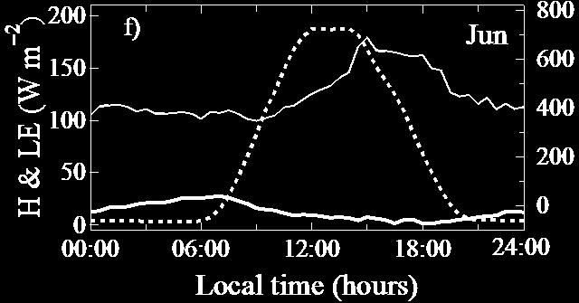
53 Figure 10. Two-year averaged monthly diurnal cycles of Rn, H, and LE. LT (local time) 40

54 Figure 11. Two-year averaged monthly diurnal cycles of water surface temperatures at different depths 41

55 Our data also indicate an exponential decrease in the diurnal wave amplitudes of water temperatures with depths and a progressive phase shift of wave amplitudes with depths (Figure 11). However, the diurnal wave amplitudes were generally small compared to the air. For example, the diurnal wave amplitudes for the water surface temperature were largest in July (5.1 C) and smallest in January (1.4 C). Small diurnal variations in the water temperature at a depth of 4.5 m were still observed, with the largest occurring in February (0.7 C) and the smallest in August (0.1 C). Relatively small wave amplitudes for water temperatures at different depths, as compared with those for soil, were attributed to the direct heating of the water by solar radiation, which penetrated down through the deep layers, as well as significant heat transfer and vertical mixing in the water layers via large eddy diffusion. It is noted that the monthly average diurnal cycles of H and LE showed no correspondence to those of Rn (Figure 10). Even when Rn was negative during nighttime, H and LE were not zero and contribute substantially to the daily means for each month. This reflected that Rn was not the direct driving force for H and LE on the diurnal timescale. However, the correspondence of large Rn and LE in the summer shows that Rn limited the energy supplied for LE in the long run. On a daily basis, the water temperature increases as the water absorbs and stores energy (Rn), creating a time lag between Rn and LE. 42

56 H exhibited diurnal sine waves, with maximums occurring in the early morning and minimums in the late afternoon. The daily maximums for H were largest in October (44.0 W m 2 ) and smallest in May (25.5 W m 2 ) for the averaged two years. The monthly average diurnal cycles of LE showed two kinds of patterns (Figure 10). In the cool season (i.e., October to March), the diurnal variations in LE roughly followed those of H. For the warm season (i.e., April to September), the bell-shaped LE developed with its maximums in the late afternoon. The daily maximum LE was largest in June (179.2 W m 2 ) and smallest in January (58.6 W m 2 ) (Figure 10). To emphasize the different controlling factors that influence diurnal variations in H and LE in the warm and cool seasons, we selected two periods to represent the winter and summer cases in 2008 for our analysis in the next two sections: January, February, and March (hereafter JFM) and June, July, and August (hereafter JJA). 43

57 Figure 12. Diurnal variations of energy fluxes and meteorological variables in the 2008 winter (January, February, and March). Note that the right axis only shows scales for LE and other variables were adjusted in their magnitudes to best match the variations in LE. z/l: the stability parameter where z is the measurement height and L is the Monin-Obukhov length). 44

58 3.4.2 Diurnal variations and controlling factors in winter (JFM) In the cool season, as represented by winter, both Rn and S o were small, with daily maximums of about 400 ~ 500 W m 2 (Figure 12a). H presented strong diurnal sine-wave cycles with relatively large amplitudes (about 35 W m 2 ), reaching daily maximum (34.1 W m 2 ) at 0600 LT (Local Time) and a minimum ( 1.5 W m 2 ) at 1700 LT. Our results indicated that these diurnal variation patterns for H were best explained by similar patterns in T w T a (R 2 = 0.94; Figure 13). Though diurnal variations for both T w and T a displayed clear sine waves, the amplitudes of T w was consistently much smaller than those of T a, leading T w T a to reach its maximum in the early morning (about LT) and minimum in the late afternoon (about LT) (Figure 12e). The daily T w T a was greater than zero for most of the time but became negative for a certain period in the late afternoon or early evening. Consequently, such diurnal variation patterns in T w T a created the ASL stratifications (reflected by the stability parameter z/l where z is the measurement height and L is the Monin-Obukhov length) that were stable for a certain period in the late afternoon and unstable during the rest of the periods (Figure 12b). The strongest unstable stratification (z/l = 0.3) of the ASL occurred in the early morning with the largest T w T a (positive), and the weakest unstable stratification (z/l = 0.1, even turning into a weakly stable stratification with a 45

59 z/l of up to 0.1) occurred in the late afternoon with the smallest T w T a (even turning into a negative value). Note that this diurnal variation in stability over water is different from over land [Stull, 1988]. The diurnal variations in LE were weak in their magnitudes and roughly followed those of H, with relatively large values in the daytime (about 55 ~ 60 W m 2 ) and small values during the late afternoon and evening (about 45 W m 2 ) (Figure 12d). In winter, the over-water air was very dry under the influence of continental air masses, and e w was also low due to the low water surface temperature. Both e w and e a exhibited little diurnal cycles (Figure 12f). As a result, diurnal variations in e w e a were fairly small, with their magnitudes varying around 0.5 kpa. However, the mechanical mixing was remarkably strong during these months, as indicated by the high U (Table 4). Under these conditions, the diurnal variations in LE were likely to be controlled more by the ASL stability than by e w e a, leading to the close correspondence between LE and z/l (R 2 = 0.67, Figure 13). The linear correlations between LE and U (R 2 = 0.02) as well as between LE and U(e w e a ) (R 2 = 0.10) were very weak (Figure 13). 46

60 UΔT ΔT U z/l UΔe Δe U z/l Figure 13. Linear regressions of the diurnal H against UΔT, ΔT, U, and z/l as well as the diurnal LE against UΔe, Δe, U, and z/l in winter Diurnal variations and controlling factors in summer (JJA) In summer, both S o and Rn were large, with daily maximums of around 650 ~ 700 W m 2 (Figure 15a), providing large energy inputs to the water. H showed similar diurnal variations as in winter but with smaller amplitudes (about 5 W m 2 smaller for the daily maximum and 5 W m 2 larger for the daily minimum). The daily T w T a was always greater than zero. Reflected by z/l, the ASL was unstable except for a short period in the late afternoon, in which the ASL was weakly stable (Figure 15b). In addition, the ASL was more unstable in the warm season than in the cool season, as indicated by the magnitudes (Figure 12b vs. Figure 15b). Note again that this diurnal cycle of the ASL stability is completely different from that over land [Stull, 1988]. 47

61 Figure 14. Diurnal variations of the surface energy fluxes and meteorological variables in the 2008 summer (June, July and August). Note that the right axis only shows scales for LE and other variables were adjusted in their magnitudes to best match the variations in LE 48

62 Diurnal variations in H were best explained by those in ΔT alone (R 2 = 0.95; Figure 14). Multiplying ΔT with U resulted in a slightly weaker correlation between H and UΔT (R 2 = 0.94; Figure 14). H was still poorly correlated with U (R 2 = 0.11, Figure 14), but better than the relationship in winter (R 2 = 0.00, Figure 13). In addition, H was moderately correlated with z/l (R 2 = 0.58; Figure 14), which was weaker than that in winter (R 2 = 0.73, Figure 13). UΔT ΔT U z/l Figure 15. Linear regressions of the diurnal H against UΔT, ΔT, U, and z/l in summer Diurnal variations in LE presented a bell-shape with its maximums (about 165 W m 2 ) in the late afternoon (Figure 15d). Both e w and e a had larger magnitudes and larger vapor pressure gradients (i.e., e w e a that varied from 1.5 to 2.2 kpa) compared with those in the winter (i.e., e w e a that varied from 0.4 to 0.5 kpa; Figure 15f). Turbulent mixing, represented by wind speeds, was sufficient (2.4 ~ 3.6 m s 1 ) with minimums at noon (Figure 15d). As a consequence, LE was considerably larger in summer than in winter in terms of its diurnal variation magnitudes. Linear regressions of LE against external forcings on the diurnal basis were applied to interpret the summertime LE diurnal cycle (Figure 16, upper panels). No linear relationship was found between LE and U (R 2 = 0.00; Figure 16a). The linear relationship between LE and U(e w e a ) 49

63 was stronger (R 2 = 0.61; Figure 16b). The strongest linear correlation existed between LE and e w e a (R 2 = 0.88; Figure 16c). It is surprising that including U with e w e a (i.e., U(e w e a )) did not improve the relationship between LE and e w e a. However, further investigations showed that the data points were distributed regularly, instead of randomly, in these linear regression plots, and these data points followed a specific temporal sequence (Figure 16, bottom panels). The LE vs. U plot basically formed a circular sequence (Figure 16d, while the LE vs. e w e a plot was close to a straight line (Figure 16e). The product of U and e w e a led to a LE vs. U(e w e a ) pattern which had a unique elliptical, temporal sequence. Figure 16. Linear regressions (upper panels) and temporal sequences (lower panels) of LE against U, e w e a, and U(e w e a ) in the summer. The arrow points toward the end of the day 50

64 This elliptical pattern was actually present in the linear regression of LE against U(e w e a ) when all summertime 30-min runs were used (Figure 23; Section 3.7), due to the overlaps of many diurnal elliptical patterns on one plot. The sharp change in LE, when U(e w e a ) approached zero, was actually the consequence of this elliptical pattern (Figure 23). It is noted from these sequences that LE was not linearly correlated with U and that the direct product of U and e w e a may not result in the best explanation for the diurnal cycles of LE. In addition, it suggests that the nonlinear relationship between LE and external forcings may be overlooked in any linear regression practice; thus one should apply this method with cautions when assessing the turbulent exchange by using Eq. (17) (Section 3.7). Based on the temporal sequences shown in Figure 16, it is speculated that external forcings such as U, e w e a, and U(e w e a ) may play relatively important roles in different time intervals to govern the temporal variations in LE. Because U and e w e a did not always vary at the same direction (i.e., increase or decrease), the phase lags between LE and U(e w e a ) were generated (Figure 14d). From 0000 LT to 0900 LT, LE closely followed the variations in U since there was little change in e w e a. After 0900 LT, e w e a increased substantially and played an increasing role in controlling the change in LE, despite a decrease trend in U (Figure 15d). This means that the mechanical mixing during the period with the weak winds was still strong enough to maintain sufficient turbulent exchange and lead to the large LE, given the presence of the 51

65 unstable ASL (Figure 15b). In the late afternoon, the combined effect of the decreased instability (even a stable ASL) and the decreased e w e a led to a decrease in LE, under the circumstance of the unchanged mechanical mixing (i.e., a little change in U) (Figure 15d). In summary, the diurnal cycle of LE was alternately affected by U and e w e a, leading to a phase lag almost always between LE and U(e w e a ). 3.5 H and LE pulses and their contributions to interannual variations in H and LE It was seen in Figures 5 and 7 that the intraseasonal variations of H and LE were superimposed with occasionally large H and LE pulses throughout the years. Therefore, analyzing the H and LE pulses (i.e., their intensity, duration, and frequency) and physical processes in producing these pulses should enable us to better understand how these H and LE pulses modulate intraseasonal, seasonal, and interannual variations in the surface energy budget Definition of H and LE pulses In previous studies on high-latitude lakes or southern ones in the cool season [Blanken et al., 2000; Liu et al., 2009], H (LE) pulses were defined as increased sensible (latent) heat flux events when the daily mean H (LE) was at least 1.5 times the value of the centered 10-day running 52

66 mean of H (LE). H and LE pulses were also found to be almost coincident to each other. Our results showed that H in summer had small magnitudes (i.e., W m 2 ; Figure 17) and experienced regular variations that could easily exceed its centered 10-day running mean while LE experienced no such variations (Figure 18). Therefore, we adopted a more reasonable definition for a H and LE pulse (hereafter pulse in short) that both H and LE should be at least 1.5 times the value of the respective centered 10-day running mean of H and LE. Based on this definition, we identified a total of 35 and 32 pulses in 2008 and 2009, covering a total of 55 and 53 days, respectively (Figures 17, 18). In addition, based on the observations from synoptic weather charts (chart sources: there were three and four cold fronts that passed over the study site during the data gap period in the cool season of 2008 and in the warm season of 2009, respectively. Therefore, it is reasonable to assume that three and four pulses were probably produced during these periods. These pulses need to be taken into account to limit errors to the minimum levels. To account for the duration of these pulses, we assumed that each pulse lasted for one day such that the total pulse days were added up to 58 and 57 days in 2008 and 2009, respectively. To account for the magnitude of these pulses, we filled the pulse gap days with the daily averages obtained from all available pulses in each season. The other days excluding pulses during the data gap period were considered as non-pulse days and were filled with the daily averages of all available non-pulse days in each season. Data gaps in the meteorological variables were also filled using the same procedure. 53

67 54 Figure 17. Daily means (lines with circles) and the centered 10-day running mean (bold lines) of H. H pulses were marked as shadows

68 55 Figure 18. Daily means (lines with circles) and the centered 10-day running means (bold lines) of LE. LE pulses were marked as shadows

69 3.5.2 Physical processes to generate H and LE pulses The frequent H and LE pulses were caused by air mass movements that were often associated with cold fronts [Blanken et al., 2000; Liu et al., 2009]. To illustrate how these cold fronts and dry air masses affect H and LE, we examined a pulse that occurred in late February of The dates on which the cold front was passing over this region was determined by comparing daily synoptic weather charts from consecutive days [Liu et al., 2011]; while the arrival time of the cold front was estimated by examining the time-series data of 30-min mean meteorological variables and H and LE fluxes [Liu et al., 2011]. Cold front Cold front Cold front February LT February LT March LT Figure 19. Daily weather maps showing the passage of a cold front in February of 2009 (local time). Star denotes the location of the study site (Chart Source: 56

70 The synoptic charts clearly showed that this cold front passed over the site on 28 February 2009 (Figure 19). The time-series data indicated that the cold front arrived at the site at approximately 0300 LT on that day, leading to a high-wind event with a rapid increase in wind speed, a dramatic decrease in temperature, and a large drop in water vapor pressure. After the cold front passage, the site was under the influences of cold and dry air masses for about five days until March 4 (see more discussion below). Before the cold front, this site was dominated by southerly winds with a mean wind speed of 5.09 m s 1 (Table 6; Figures 20, 21). These air masses were warm and humid (T a = 16.6 C, RH = 0.71, e w = 1.34 kpa), passing over the relatively cooler water surface (T w = 12.1 C), leading to a negative T w T a ( 4.5 C) and small e w e a (0.07 kpa) (Table 6; Figure 21). Consequently, H was small and even negative in the afternoons and evenings ( 20.8 W m 2 ). LE was also suppressed and close to zero for most of the time ( 2.6 W m 2 ) (Figure 21; Table 6). Table 6. Comparisons of the energy fluxes and meteorological variables within and outside a pulse event in February The dates for outside of the pulse event were averaged over 3 days before and 3 days after the event. The duration for the event was averaged over 5 days. So Rn LE H U T a T w ΔT RH e a e w Δe W m 2 W m 2 W m 2 W m 2 m s 1 C C C kpa kpa kpa Outside Within Difference

71 After the cold front s passage, wind directions shifted immediately from the south to the north, with an increase in wind speeds from 5 m s 1 to 11 m s 1 and then a decrease steadily towards the pulse end (Table 6; Figures 20, 21). Meanwhile, T a decreased by 11 C while e a decreased by 0.76 kpa after the passage of the cold front (Table 6; Figure 21). Due to the large heat capacity of water, T w only decreased by 0.4 C and e w decreased by 0.03 kpa. As a result, large gradients of temperature (T w T a ) and vapor pressure (e w e a ) between the water surface and the overlying air were produced (T w T a = 6.1 C, e w e a = 0.80 kpa). Resulting from the combined effect of the enhanced mechanical mixing, increased vertical gradients (T w T a, e w e a ), and enhanced instability (as reflected by T w T a ), H and LE were significantly promoted during the pulse days (i.e., H increased by 71.1 W m 2 ; LE increased by W m 2 ) (Table 6; Figure 21). Note that the increase in Rn was a result of the cloudless days associated with the high pressure system after the cold front passage (Figure 21). Figure 20. Comparisons of wind directions and wind speeds within and outside a H and LE pulse event in February of

72 H and LE pulse event Wind direction (degree) Air pressure (kpa) Figure 21. Changes in surface energy fluxes and meteorological variables after a cold front in February

73 3.5.3 Contributions of H and LE pulses to the surface energy budget In general, there were 36 ~ 38 pulses per year, covering 57 ~ 58 days (16% of 365 days; Table 7). It was evident that pulses occurred more often in the cool season, covering 22% of the days, than in the warm season, covering 9% of the total days. To estimate the contribution of H and LE in pulse days to the overall H and LE, both the duration and intensity of the pulses were taken into account using Eq. (16) Flux( PS) Days( PS) Ctrn. Flux( PS)% = 100% (16) Total( Flux) where Ctrn.Flux(PS)% is the contribution of the flux in percentage to the overall flux, Flux(PS) is the averaged daily mean of the flux during the pulse days, Days(PS) is the pulse days with H and LE pulses. These similar processes were also applied to estimate the contribution of H and LE from the non-pulse days (i.e., Ctrn.Flux(NPS)) to the overall flux. Thus, Flux(NPS) and Days(NPS) denote the daily mean flux and the non-pulse days in each season. When averaged over the two years, we estimated that H(PS) contributed to 50% of the annual H, reflecting their significant contributions to the overall H (Table 7). On the annual basis, H(PS) was much larger (50.9 W m 2 ) than H(NPS) (9.4 W m 2 ), with the annual mean H m of 15.9 W 60

74 m 2 (hereafter the subscript m denotes the mean of the quantity under consideration for the discussed period). In the warm season, H(PS) had small magnitudes (46.6 W m 2 ) and contributed to less than half (30%) of the H m-warm, indicating that H m-warm was more controlled by H(NPS). In the cool season, H(PS) had large magnitudes (52.7 W m 2 ) and contributed to more than half (68%) of the H m-cool, indicating that H m-cool was more controlled by H(PS). Moreover, the smaller H(NPS) in the cool season (7.1 W m 2 ) than in the warm season (11.4 W m 2 ) indicates that H and LE pulses enhanced more turbulent exchanges in the cool season in spite of the smaller baseline, leading to larger H m-cool (17.2 W m 2 ) than H m-warm (14.6 W m 2 ) (Table 7). Table 7. Two-year averaged daily mean H and LE during the periods of non-pulse days (NPS) and the periods of pulse days (PS) in the cool season, warm season, and the entire year; Ctrn. denotes contribution Cool season Warm season Annual Variable Units Overall NPS PS Overall NPS PS Overall NPS PS Days Days Ctrn. Days 100% 78% 22% 100% 91% 9% 100% 84% 16% H W m Ctrn. H 100% 32% 68% 100% 70% 30% 100% 50% 50% LE W m Ctrn. LE 100% 52% 48% 100% 83% 17% 100% 72% 28% Averaged over the two years, LE(PS) contributed to 28% of the annual LE, reflecting their substantial contributions to the overall LE (Table 7). On the annual basis, LE(PS) (146.9 W m 2 ) was about twice LE(NPS) (70.9 W m 2 ), with the annual mean LE m of 82.9 W m 2. In the cool 61

75 season, LE(PS) contributed to about half (48%) of LE m-cool, and LE(PS) was at least three times LE(NPS), indicating that LE m-cool was more controlled by LE(PS). All the LE(PS), LE(NPS), and LE m-warm in the warm season were larger than those in the cool season, indicating the significant contribution of warm-season LE to the overall LE. LE(PS) contributed to a small portion (17%) of the overall LE m-warm in the warm season (Table 7), indicating LE m-warm was more controlled by LE(NPS). 3.6 Interannual variations The overall Rn was slightly larger in 2008 (109.4 W m 2 ) than in 2009 (106.1 W m 2 ) (Table 8). Both H and LE were about 10% larger in 2008 (H m = 16.6 W m 2, LE m = 86.8 W m 2 ) than those in 2009 (H m = 15.2 W m 2, LE m = 78.9 W m 2 ). Then what caused these large interannual variations in H and LE despite the small differences in available energy (Rn) and no changes in T w? We hypothesize that seasonal variability in high-wind events and the meteorological properties associated with the H and LE pulses modulated heat and water vapor transfer, leading to larger H m and LE m in 2008 compared to those in

76 Table 8. Daily means of the energy fluxes and meteorological variables during overall days, non-pulse days (NPS), and pulse days (PS) for the cool and warm seasons as well as for the whole year in 2008 and 2009 Cool season Warm season Annual Variable Unit Year Overall NPS PS Overall NPS PS Overall NPS PS Pulse Days Rn W m H W m LE W m U m s T a C T w C e a kpa e w kpa T w T a C e w e a kpa

77 3.6.1 Factors modulating interannual variations in H and LE In general, the overall means of T a for both the cool and warm seasons of 2008 were lower than those in 2009, leading to slightly lower annual mean T a (17.9 C) which was 0.2 C lower in 2008 than that in 2009 (Table 8). In correspondence to Rn, T w was higher in the cool season but lower in the warm season in 2008 than that in 2009, leading to a similar annual mean T w (20.3 C). The air was cooler in 2008 than in 2009; while the water had the same temperature in both years, leading to larger T w T a in 2008 (2.4 C) than 2009 (2.3 C) (Table 8). Consistent with T w, e w was very close for the two years, while e a was lower in all seasons of 2008 (i.e., the annual mean e a = 1.55 kpa) than those of 2009 (i.e. the annual mean e a = 1.59 kpa), leading to a slightly larger e w e a in In summary, the air was cooler and drier in all seasons of 2008 than 2009, while the water experienced similar annual means in both years, leading to a slightly larger T w T a and e w e a in 2008, as compared with Nevertheless, T w T a and e w e a were smaller in the warm season of 2008 than in In the warm seasons, Rn and H were fairly close in 2008 (Rn = W m 2, H = 14.6 W m 2 ) to those in 2009 (Rn = W m 2, H = 14.6 W m 2 ) and there was small difference in LE (110.3 W m 2 in 2008 vs W m 2 in 2009) (Table 8). Thus the major interannual variations must originate from the cool season. It was shown that the overall Rn, H, and LE in the cool season of 2008 (Rn = 62.2 W m 2, H = 18.7 W m 2, LE = 63.2 W m 2 ) were 13%, 19%, and 24% larger 64

78 than those in the cool season of 2009 (Rn = 55.2 W m 2, H = 15.7 W m 2, LE = 50.8 W m 2 ) (Table 8). Further investigations showed that both non-pulse days and pulse days in the cool season experienced large interannual variations. During the non-pulse days in the cool season, Rn(NPS) was 20% larger in 2008 (66.3 W m 2 ) than in 2009 (55.1 W m 2 ), indicating more available energy for the cool season of 2008 than in 2009 (Table 8). This additional energy explained part of the variations in LE(NPS), which was 37% larger in the cool season of 2008 (43.9 W m 2 ) than the cool season of 2009 (32.1 W m 2 ). H(NPS) was 27% larger in the cool season of 2008 (7.9 W m 2 ) than the cool season of 2009 (6.2 W m 2 ). Since H and LE during the non-pulse days were more correlated with T w T a and e w e a, respectively (Section 3.4), the magnitudes of H(NPS) and LE(NPS) were indicators of the over-water meteorological conditions. Therefore, we expect larger T w T a and e w e a in the cool season of 2008 than in In fact, our calculations indicated that the mean T w T a and e w e a were 1.2 C and 0.57 kpa, respectively, during the non-pulse days in the cool season of 2008 and 0.8 C and 0.48 kpa, respectively, during the non-pulse days in the cool season of 2009 (Table 8). In addition, the higher T w in the cool season of 2008 (14.4 C) than in 2009 (14.0 C) indicates that more heat was stored in water to provide primary energy source for H and LE in both non-pulse days and pulse days. 65

79 During the pulse days, Rn(PS) was actually smaller in the cool season of 2008 (47.9 W m 2 ) than the cool season of 2009 (55.7 W m 2 ) (Table 8). However, both H(PS) and LE(PS) were larger in the cool season of 2008 (H(PS) = 55.7 W m 2, LE(PS) = W m 2 ) than the cool season of 2009 (H(PS) = 49.6 W m 2, LE(PS) = W m 2 ). It was known that H and LE were associated with the intensity, duration, and frequency of high-wind events [Liu et al., 2011]. Given that 2008 and 2009 had similar numbers of H and LE pulses, we expected the larger H(PS) and LE(PS) would imply that the high-wind events were stronger in the cool season of Our results showed that during the pulse days, U was 13% larger in the cool season of 2008 (5.2 m s 1 ) than the cool season of 2009 (4.6 m s 1 ). The slightly larger T w T a and e w e a were also presented during the pulse days of the cool season of The combination of these factors promoted H and LE exchange during the pulse events more in the cool season of 2008 than in the cool season of These exchange extracted more energy stored in the water, as reflected by the lower T w during the non-pulse days in the warm season of 2008 (26.5 C) than in 2009 (26.9 C). Moreover, it was shown that pulses significantly contributed to the total interannual variations in H and LE fluxes between 2008 and For H, 80% of its interannual variations were attributed to the interannual variation in pulses, while the remainder 20% was from those in non-pulse days. For LE, 40% of its interannual variations were attributed to those in pulses, 66

80 while the remainder 60% was from non-pulse days. In summary, the interannual variations in the surface energy budget between 2008 and 2009 was mainly caused by the variations in the cool season, in which 2008 had more available energy during the non-pulse days and experienced stronger high-wind events during the pulse days. These results suggest that the interannual variations in water surface energy fluxes are strongly dependent upon their variations in cool seasons, due to significant modulation by H and LE pulses. These H and LE pulses are largely determined by the intensity, frequency, and duration of high-wind events associated with synoptic weather conditions. Several studies have shown that cyclone activities have changed in the past decades due to climate change [McCabe et al., 2001; Teng et al., 2008]. Future changes in the intensity, frequency, and duration of cold front activities and the associated high-wind events due to climate change would likely modify the water surface energy fluxes in the cool season and thus alter their annual and interannual variations. It is interesting to know whether climate change will intensify or weaken the water surface energy fluxes because both the meteorological properties associated with high-wind events during H and LE pulse days and the weather conditions during non-pulse days have significant influences on the overall changes. Future studies should pay attention to these questions since evaporative loss of fresh water from inland water bodies, a component of the surface energy budget, could have significant implication for water resource managements through the process of evaporation. 67

81 3.6.2 General statistical analysis of winds for 2008 and 2009 Wind rose diagrams enable us to study influences of wind speeds and directions affecting the surface energy exchange (Figure 22; Table 9). The radius of the rose plot is the percentage that winds with certain speeds are within a given direction range. The different colors indicate the wind speed ranges as explained in the legend. In this study, an increment of 90 degree in wind directions and an increment of 2 m s 1 in wind speed were used. All winds were categorized into west, north, east, and south. Figure 22. Wind rose diagrams for 2008 and The radius of the rose plot is the percentage that a wind speed value is within the given direction range. The different colors indicate the wind speed ranges as explained in the legend. In this study, an increment of 90 degree in wind directions and an increment of 2 m s 1 in wind speed were used 68

82 In the cool season of 2008, the northerly winds were predominant and comprised up to 37% of the annual statistics. It was also apparent that there were more high-wind events in 2008, as reflected by more than 20% of winds at speeds higher than 6 m s 1. In contrast, the southerly winds were predominant in 2009, consisting of 32% of the annual statistics, with a large percentage of speeds between 2 to 6 m s 1 (Figure 22; Table 9). In 2009, the northerly winds accounted only for 23% of the annual statistics, with 15% of which at speeds higher than 6 m s 1. It is speculated that the winds blowing from different directions were affected by various synoptic weather systems such as anticyclones and cyclones, bringing in air masses with different meteorological properties to this region. These different air masses provide distinctive atmospheric forcings and temporal variations on synoptic scales, affecting exchange processes of H and LE over the water surface. In general, winds from the continent (i.e., west, north, and east) brought in cool/dry air masses, which enhanced temperature and humidity gradients (i.e., T w T a, e w e a ), while southerly winds brought in warm/humid air masses, which reduced the gradients. For example, it is shown in Table 9 that southerly winds were generally associated with lower T w T a and e w e a than the winds from other directions. As a consequence, H and LE were generally promoted under the influence of continental winds, while suppressed under the influence of southerly winds (i.e., 69

83 smaller H and LE for southerly winds in both years, Table 9). Specifically in winter, continental winds promoted LE due to the enhanced mechanical mixing (i.e., higher wind speeds). Therefore, interannual variations in wind directions and wind speeds are likely to contribute partly to interannual variations in H and LE in this region, as more continental winds with higher wind speeds resulted in larger T w T a and e w e a, hence larger H and LE in 2008 than in Table 9. The 30-min means of components of the surface energy budget and meteorological variables from the west (W), north (N), east (E), and south (S) in 2008 and 2009 WD U H LE e w e a T w T a % m s 1 W m 2 W m 2 kpa C W 13% 13% N 37% 23% E 22% 19% S 25% 32%

84 3.7 Mechanisms controlling turbulent exchanges It is well known that LE over water surface depend largely on the vertical gradient of vapor pressure at the water-air interface (i.e., e w e a ) as well as on intensity of turbulent mixing [Bonan, 1995; Hendersonsellers, 1986; Hostetler and Bartlein, 1990]. In numerical models, the mass transfer method (Eqs. (17), (18)) was used extensively for estimating the LE over lakes and reservoirs [Blanken et al., 2000; Garratt, 1992; Stull, 1988] H = ρ C C U ( T Ta ) (17) a P H w LE = LC U ( e e ) a (18) E w where ρ a is the air density (kg m 3 ), C P is specific heat of air (J C kg 1 ), L is latent heat of vaporization, U is the horizontal wind speed (m s 1 ) at the reference height in the ASL, T w and T a are the water surface layer temperature ( C) and the air temperature ( C) at the reference height, e w and e a are the vapor pressure (kpa) at the water surface and the reference height, and C H and C E are the bulk transfer coefficients for heat and moisture, respectively [Garratt, 1992; Liu et al., 2009; Stull, 1988]. Previous studies have found good match between estimation using U(e w e a ) and the measured LE, as well as between estimation using U(T w T a ) and the measured H on a daily basis in the northern lakes [Blanken et al., 2000; Nordbo et al., 2011] or in the cool season in southern lakes [Liu et al., 2009]. In this study it was found that U and e w e a have separate or joint impacts on 71

85 LE. Thus it was expected that U and e w e a may play different roles in governing turbulent exchange of LE on different timescales and during different seasons. Our results showed that based on the correlations between half-hourly LE and U(e w e a ), the data points were concentrated around the 1:1 line in the cool season (R 2 = 0.79), while widely scattered in the warm season (R 2 = 0.47) (Figure 23). For H, the higher correlations were also present for the cool season (R 2 = 0.84) than the warm season (R 2 = 0.76). Overall, the correlation coefficients were larger for H than LE annually or seasonally (Figure 23). What processes, then, caused these two distinctive correlation patterns for these two seasons? Overall year Cool season Warm season Figure 23. Relationships between half-hourly H and U(T w T a ) over the year, in the cool season, and in the warm season (upper panels). Relationships between half-hourly LE and U(e w e a ) over the year, in the cool season, and in the warm season (lower panels). All available data points in 2008 and 2009 were used 72

86 The nonlinear interaction between U and e w e a on LE requires a detail analysis about their relationships with LE. Therefore, we divided e w e a (hence denoted as Δe) into a number of small, continuous ranges, performed linear regressions of half-hourly LE data against U and Δe in each Δe range, and then discussed the possible causes that led to better relationships between LE and U in some specific Δe ranges. Due to the distinct intraseasonal patterns in the winter (i.e., January, February, and March) and summer (i.e., June, July, and August) (Figure 24), the analyses were conducted separately for these two seasons. Δe Δe Figure 24. Scatter plots of U against Δe on the diurnal timescale in the winter and summer In general, our results indicated that LE had poor correlations with Δe in each Δe range in both the winter and summer (R 2 0.2; Figures 25, 26). In contrast, LE was generally in good linear correlation with U in each Δe range, with the slope being larger as Δe increased (Figures 25, 26). 73

87 Δe also affected LE but in a different way. When we averaged all LE points to obtain one averaged value for each Δe range and make the same average from U and Δe, and plotted these means against the averaged Δe in Figure 27, we found a very strong correlation between the averaged LE and the averaged Δe (R 2 = 0.94). In winter, Δe was small (0~1.6 kpa) and thus was the limiting factor for LE while U was large (Figure 25). Both U and Δe increased in winter due to the increased numbers of windy days with dry and cold air masses passing over water, leading to stronger linear correlations between LE and UΔe as well as between U and Δe (Figure 27). It is also noted that when Δe was very small (i.e., Δe 0.3 kpa), LE was also around zero. When Δe became large, the correlation coefficients between LE and U increased. This indicates that when the vapor pressure gradient over water was small, it acts as a limiting factor that even large mechanical mixing (high U, up to 15 m s 1 ; Figure 25) would not promote LE. When Δe became larger, LE was not limited by Δe and thus was more associated with U than Δe (Figures 25). However, the correlation coefficients between LE and U with the increased Δe approached their maximums when Δe was about 1.0 kpa, and then even decreased when Δe was greater than 1.0 kpa. 74

88 R LE vs. Δe R LE vs. U Figure 25. The linear relationship between LE and Δe (upper panels) or U (middle panels) in designated Δe ranges and their correlation coefficients (bottom panels) in winter 75

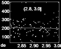
89 LE vs. Δe LE vs. U Figure 26. The linear relationships between LE and Δe (upper panels) and between LE and U (middle panels) in designated Δe ranges and their correlation coefficients (bottom panels) in summer 76

90 In summer, Δe was relatively large (1 ~ 3.7 kpa) while U were relatively small and acted as a limiting factor for driving LE. Both U and Δe exhibited strong diurnal cycles and sometimes varied at different directions (Figure 26). It is noted that averaged over all Δe ranges, U had a robust negative linear relationship with Δe (R 2 = 0.90; Figure 27). When U and Δe did not change at the same direction during a day; the variations in LE were not well quantified by UΔe, leading to the weakened correlation relationship between LE and UΔe (Figures 27) In summary, LE was under the joint influences of Δe and U, with Δe determining its magnitude and U determining its variations. Figure 27. Relationships of LE, U, and Δe for different Δe ranges in winter and summer. All values are averaged in the same Δe range. It shows that LE is strongly related with Δe between ranges. Also, U is positively correlated with Δe in the winter, and negatively correlated with Δe in the summer 77

91 3.8 Comparison of the surface energy budget with high-latitude northern lakes In this section, the annual and seasonal surface energy budget over a large low-latitude water body, the Ross Barnett Reservoir (hereafter RBR, in this study) and over a typical large high-latitude lake, the Great Slave Lake (hereafter GSL), were compared and analyzed. We adopted the eddy covariance data over GSL which were measured in 1999 and reported by Blanken et al. [2000] and Rouse et al. [2003]. RBR was ice-free throughout the year, while GSL was ice-free for 192 days on average in a year, and covered with ice for an average of 173 days (Table 10). The GSL ice-free season was typically between June 1 15 and December 15 to January 1 [Rawson, 1950]. H and LE were only available for the ice-free season. In addition, the area and mean depth for GSL were much larger than RBR (Table 10), leading to larger water heat storage capacity for GSL Comparison of the annual mean surface energy budget and cumulative evaporation Previous studies have focused on the evaporation regime over high-latitude lakes [Blanken et al., 2003; Blanken et al., 2008; Blanken et al., 2000; Rouse et al., 2003; Rouse et al., 2008; Rouse et al., 2005; Schertzer et al., 2003]. The annual mean LE and cumulative evaporation (hereafter cume) in GSL and RBR are listed in Table 10. Note that the annual mean LE (unit: W m 2 ) and cume (unit: mm) were linked through Eq. (19) 78

92 LE cume = Days L 10 3 (19) where L is the latent heat of vaporization for water, Days are the ice-free periods for the lakes. On an annual basis, it is evident that RBR has much larger LE and cume (i.e., annual mean LE = 83 W m 2, cume = 1156 mm) than GSL (i.e., annual mean LE = 59 W m 2, cume = 432 mm) (Table 10). This indicates that both LE and evaporation have larger magnitudes for RBR than in GSL, suggesting that evaporative water loss from low-latitude lakes are likely to be more significant compared with those in high-latitude lakes. In addition, Rn was smaller in GSL (i.e., Rn in 2009 <101 W m 2 ) than in RBR (i.e., annual mean Rn = 108 W m 2 ), indicating less energy input to the water surface. H was likely to be larger in GSL (i.e., >22 W m 2 ) than in RBR (i.e., annual mean H = 16 W m 2 ) (Table 10), indicating more heat was transferred into the atmosphere through H in high-latitude lakes than in RBR. Interannual variations were also evident for both water bodies. However, in RBR which is ice free, interannual variations in H and LE are mainly caused by interannual variations in H and LE pulses (e.g., their durations, intensity, and frequency) as well as Rn. On the contrary, the final ice breakup date is found to be the most important factor affecting the interannual variations in the surface energy balance over GSL [Rouse et al., 2005]. Earlier ice breakups lead to more energy absorption of solar radiation which reaches its maximum in June, earlier heating of the lake, and 79

93 hence sooner the changes from stable to unstable over-lake ASL regimes. In addition, earlier breakups are highly likely related to longer ice-free periods, resulting in larger cume in GSL (Table 10). Table 10. Comparison of the annual mean LE and annual cumulative evaporation (cume) over a low-latitude water body (in this study) and a high-latitude lake (GSL). All studies used direct measurements from eddy covariance systems. Both LE and cume were apparently larger over RBR than over GSL. Ref reference sources for studies: 1) Blanken et al. [2000]; 2) Rouse et al. [2003]; 3) Oswald and Rouse [2004]; 4) the present study. Location Area Mean Depth Ice-free Period Days Rn H LE cume Ref km 2 m W m 2 W m 2 W m 2 mm Great Slave Lake (GSL) N, Jun 13 Dec W 1 Jun Jan Jun 13 Dec <101 > Jun 9 Dec Mean Ross Barnett Reservoir (RBR) N, Annual W Annual Mean Comparison of seasonal variations in the surface energy budget Seasonal variations in the surface energy budget were significantly different between GSL and RBR. At the beginning and the end of the year, solar radiation was close to zero over GSL while it was approximately 100 W m 2 over RBR, indicating less energy input to the water surface for high-latitude lakes in the winter (Figure 28). As the months progressed, solar radiation shared 80

94 similar bell-shapes over both water bodies. Rn over GSL was negative during the roughly first four months and lasted two months of the year, while Rn over RBR remained positive across the year. Interestingly, Rn did not increase to exceed zero until May in GSL, while it generally followed solar radiation over RBR (Figure 28). This lag in increasing and in achieving positive Rn was controlled by the extent of ice melt over the lake [Rouse et al., 2005]. GSL So Rn RBR So Rn Figure 28. Comparison of annual radiation cycles between a large high-latitude lake (left, GSL) and a large low-latitude water body (right, RBR). The 5-day running means were presented. The left GSL plot was adopted from Rouse et al. [2005]. Seasonal variations in LE, H, and z/l over GSL exhibited significantly different patterns from those of RBR (Figure 29). In general, LE and H over GSL were similar and smallest at the beginning of the ice-free season, increased gradually as the months progressed into winter, and reached maximum before the water was covered with ice. Since Rn decreased after its maximum in June and July, which corresponded to the beginning of the ice-free season, both LE and H were apparently disconnected with Rn. In fact, the seasonal variations in LE and H over GSL 81

95 were found to be best explained by the seasonal variations in z/l over the water surface [Blanken et al., 2000; Rouse et al., 2003]. According to z/l, the ice-free season can be divided into two stages: the heating stage and the cooling stage. The heating stage lasted from the final ice breakup in June till mid- to late August, during which T w was smaller than T a, leading to a negative temperature gradient and a stable atmosphere (reflected by positive z/l) over the water (Figure 29). LE and H were suppressed during this stage and Rn was mainly used to heat the water. The cooling stage started thereafter till its freeze up, during which T w exceeded T a, creating a positive temperature gradient and an unstable atmosphere (reflected by negative z/l, Figure 29), and leading to largely promoted LE and H. During the cooling stage, Rn was small and LE and H were large, indicating the energy previously stored in the water in the heating stage was released into the atmosphere in the form of LE and H. Note that the magnitude of LE during the cooling stage of GSL was close to that in the warm season of RBR. H was much larger during the cooling stage of GSL than in the cool season of RBR. The absolute magnitudes of z/l over GSL generally had larger magnitudes, whether positive or negative, than those over RBR. However, z/l was typically negative over RBR throughout the year, indicating typical unstable over-water ASL conditions over low-latitude water bodies. 82

96 Great Slave Lake (GSL) Ross Barnett Reservoir (RBR) LE (W m 2 ) a) b) c) z/l H (W m 2 ) Figure 29. Comparison of the annual patterns of a) the latent heat flux (LE), b) the sensible heat flux (H), and c) the atmospheric surface layer stability (z/l) between a low-latitude lake (present study) and a high-latitude lake (the Great Slave Lake). The patterns of the daily means (thin lines) are illustrated by 10-day running means (thick lines). Plots for the Great Slave Lake were adopted from Blanken et al. [2000]. Large LE and H pulses were also evident for GSL during the ice-free period. Previous studies found these pulses were due to strong wind activities which enhanced turbulent exchanges. This shows that the surface energy budget over the high-latitude lakes was also influenced by high-wind events, similar with this low-latitude water body as discussed earlier in this study. 83