An Analysis of the Kansas Halloween Flood of 1998

Transcription

1 An Analysis of the Kansas Halloween Flood of 1998 Nicole Schiffer Department of Atmospheric and Oceanic Sciences University of Wisconsin, Madison ABSTRACT According to radar estimates, over eight inches of rain fell near Wichita, Kansas, between 00Z on 31 October and 12Z on 1 November A National Oceanic and Atmospheric Administration report cited up to ten inches of rain in some areas of south-central and southeastern Kansas. This precipitation came in three pulses: the first two very similar in forcing and appearance and the last quite different but more persistent. All were related to an upper-level low and two associated surface cyclones. The first two spawned in eastern New Mexico and moved northeast into Kansas. The last formed near Kansas as part of the main comma-head of the cyclone. The first two pulses propagated northeastward with the mid-level steering flow. The last pulse somewhat propagated with the steering flow, but later turned into more locally produced precipitation north of a cyclone. These three pulses, which accounted for most of the flooding rains but not all, took nearly two days to pass, and most of it was quite heavy. Flood analysis is an extremely complicated issue that involves topography, soil permeability, and precipitation. Some rivers flooded due to a combination of moderate to poor soil permeability and copious amounts of rain, while the Marias Des Cygnes in particular flooded primarily because of very poor soil permeability under moderate rain accumulations. 1. Introduction Most of the rain that resulted in the Kansas Halloween flood of 1998 fell over a day and a half. The highest radarestimated totals near Wichita topped eight inches. Many area rivers crested above flood stage by several feet. The Marais Des Cygnes River went 15.3 feet above its 28-foot flood stage as measured in Osawatomie, KS, and remained above flood stage for six days (storm reports). Many rivers also broke their crest records: the Arkansas River at Derby and Arkansas City, the Whitewater River at Towanda, and the Cottonwood River at Plymouth and Florence. The Walnut River broke its record at Arkansas City by over three feet. Although widespread flooding is generally not considered as dramatic as a tornado or even lesser severe weather, it can still cause quite a bit of damage due to its scale. In addition to setting hydrological records, the floods also caused millions of dollars of damage across several counties, the hardest hit of which was Butler County ($10 million), followed closely by Cowley County ($8 million). The Cowskin Creek was cited by several sources as one of the more damaging flooded rivers. Fortunately only one human death was reported, though many livestock were also lost. Floods are a complex phenomenon. In this particular case, most of the flooding was caused by the abundant rainfall over the Halloween weekend of The rain was caused by a stationary front initially, and then a cyclone moving northeastward through the area. In combination with low soil permeability, many regional rivers

2

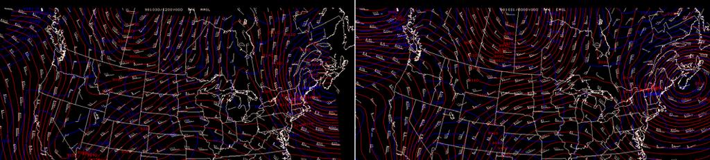
3 overflowed their banks. In order to assess the hypothesis, this report will analyze the causes of the copious amounts of rainfall that caused the Halloween flood and why certain rivers overflowed their banks using multiple data sources. The remainder of this paper will be organized as follows: Section two will outline the data sources used to perform the analysis. Section three will summarize the synoptic situation during the event, and section four will discuss the mesoscale causes and topography. Conclusions of this study will be summarized in section five. 2. Data For a calamity involving so many scales, a variety of data sources must be used to properly evaluate the event. The main sources used for the synoptic overview were isobaric observations at several mandatory levels derived from rawinsondes, supplemented by RUC model data, national radar composites, and GOES-8 satellite imagery in the 10.7μm infrared channel, the water vapor channel, and in the visible. The visible imagery has 1km resolution, and the other two channels have 4km resolution. For the mesoscale analysis the full rawinsonde profiles were added to the repertoire. The Kansas Water Office provided a map of the drainage areas for major rivers in Kansas, which will be used to identify why certain rivers overflowed more than others. Analysis will begin at 12Z on 30 October 1998 because that was the time at which the first pulse formed in New Mexico. Data ended at the end of 1 November 1998, so most analysis will end at that time, though river stage records from the National Weather Service storm reports will continue for days afterward since some rivers remained above flood stage after the rain stopped. Surface observations were also only available on 30 October, so later data will not be included. 3. Synoptic Overview Despite that this flood was a largely mesoscale event, synoptic conditions played a very significant role. At 12Z on 30 October a 300hPa trough was over southern California with a surface inverted trough and associated 1003hPa low pressure center over central Arizona, the usual westward tilt of a cyclone with height in the midlatitudes (figure 1a). Convection was just starting in east-central New Mexico east of the inverted trough along the tail end of a stationary front draped from eastern New Mexico to western Arkansas. Twelve hours later the same system was just west of Wichita, KS, and a new group of storms in New Mexico was only a couple of hours old (figure 1b). The stationary front extended through south-central New Mexico. At 300hPa the cyclone was a bit more cut off from the westerly flow and located in southeast Arizona. The surface low was still dispersed but the minimum pressure decreased to 1002hPa and moved into southwest New Mexico. Moderate rain was reported in Wichita. By 12Z on 31 October the upperlevel low moved into central New Mexico and the surface low weakened to 1004hPa over southeast New Mexico (figure 1c). The upper-level feature was starting to overrun the surface feature. The stationary front extended from north-central Colorado into central New Mexico and then took a sharp eastward turn through central Arkansas. The curve of the front actually looked like a bowl full of thunderstorms from eastern

4 Colorado through all of Kansas and south into the panhandle of Texas. Wichita reported heavy rain. At 00Z on 1 November the stationary front still splits Colorado into eastern and western halves and runs from eastern Oklahoma into central Arkansas, but the middle portion broke into a cold front from central Oklahoma and running southwest through Texas (figure 1d). A shortwave inverted trough within the main inverted trough was becoming the main axis of the trough. The surface pressure center was on the Mexico-Texas border and disappearing from consideration with regard to the Kansas flood. A line of stronger storms formed behind the cold front and the final pulse of rain in Wichita was well in progress. The upper-level cyclone moved east into central New Mexico, though it no longer seemed to be connected to a distinct surface feature. Thunderstorms were reported in Wichita. Over the next twelve hours a very weak but distinct surface low of 1006hPa had reformed in southeast Oklahoma at the north end of the cold front that was apparent 12 hours earlier (figure 1e). It is likely that the new surface low formed when the upper-level cyclone passed over the baroclinic zone that became the cold front and deformed the zone. The cold front was aligned south-southwest and the stationary front was still visible running southeast from the low. A stronger line of storms ran along the cold front, through the surface cyclone center, and north through the trough axis. The 300hPa feature was located just west of the New Mexico- Texas border, once again creating the westward-tilted cyclone structure with a new surface low. Wichita did not report any precipitation but was completely surrounded by radar echoes. It is still raining around Wichita by 00Z on 2 November, though again Wichita did not report any precipitation. The rain was nearly over. The surface cyclone at 1003hPa was more or less north of its position 12 hours ago over the Kansas-Oklahoma border. The fronts were irrelevant for Kansas, but the main cloud head of the cyclone was dropping its last bit of rain on Wichita. It was occluding and beginning to die. Based on the previous track of the upper-level low it was nearly vertically stacked over the surface feature again, further indicating the decay of the surface feature. Several of the rivers and streams near Wichita have already risen beyond flood stage and some had even crested. 4. Mesoscale Analysis a. First and Second Pulses According to Rauber, et al (2002), it is quite common that precipitation repeatedly forms along a stationary front and propagates northeastward with the steering flow. Figure 2 shows a conceptual model of this situation. The moist air moves from the warm side of the front to the cool side, overrunning the cool air (figure 3). This can cause enough lift to initiate storms. This was the setup for the first

5

6 portion of this case, through the first two pulses. The first pulse of rain was born around 12Z on 30 October in eastern New Mexico at the western edge of a very moist area (figure 4a). As it crossed the eastern New Mexico border around 14Z on 30 October, the southwestern cell. The anvil of the southwestern cell masked any signal from the stronger cell. The lack of separation between the two was likely also affected by the lower resolution of infrared imagery (4km versus 1km in the visible). The situation is much the same in the water vapor channel. maximum reflectivity was 60-65dBz in each of two main cells, arranged along a southwest to northeast line. They are joined by a small area of reflectivity mostly less than 30dBz. There is a convective plume in the visible imagery associated with the stronger, northeastern of the two cells (figure 4b). The maximum cloud top temperature observed by the infrared channel was 214K. Compared to the Amarillo sounding and assuming these temperatures were fairly close to the cloud top temperatures, the approximate cloud top height was 12000m in the By 03Z on 31 October the complex had reached Wichita and the maximum reflectivity was reduced to around 50dBz, but the area of 35-40dBz was greatly expanded (figure 4c). While this level of reflectivity does not usually indicate severe weather, it can mean a high hourly rain rate. There were no longer two distinct cells. Unfortunately, satellite confirmation was unavailable since visible imagery was not available at this time, and the infrared and water vapor channels could not distinguish individual cells in close proximity. The infrared imagery does, however, indicate

7 cloud top temperatures of 212K, or 12500m. This was above the tropopause on the sounding, so it probably was the overshooting top of a convective plume. The cloud tops of the surrounding area are closer to 11000m, or near the tropopause. Even though it looked like it was north of the Kansas border in the satellite image, it probably corresponds to the stronger cells in Oklahoma since the satellite was looking at the clouds from the south rather than from directly above. The cloud tops associated with the precipitation over Wichita are more on the order of 220K, or 10800m. These more uniform cloud tops that are still near the tropopause but have no overshooting tops are indicative of dying cumulonimbi. Other reasons discussed later also support this view. The second pulse was also born in central to eastern New Mexico shortly before 00Z on 31 October, but started as numerous smaller cells as compared to the first pulse that started as two larger cells (figure 4a). This does not seem to have anything to do with the Richardson number because it changed only negligibly during the intervening time. The highest reflectivity of these cells was above 65dBz and had a weak enhanced-v associated with it in the infrared image, which suggest a possibility of hail (though none was reported). The corresponding cloud top heights were less than 210K, which corresponded cloud top heights near 15000m. It makes sense that the cloud tops were much higher given the higher reflectivity since a stronger updraft, which causes the overshooting top, can keep larger particles suspended. Between radar and satellite, it is obvious that these storms were very convective at 03Z. Over the next seven hours the reflectivities generally decreased and merged along with the cloud top heights. It entered the Wichita area around 10Z on 31 October, shortly after the first pulse passed (figure 4b). This pulse moved much faster than the first one, since it only took 10 hours to get from New Mexico to Wichita, whereas the first one took 15 hours. An increase in mid-level winds between 12Z on 30 October and 00Z on 31 October, between the births of the two storms, was likely the cause of the differing propagation speeds. On the 10:15Z infrared satellite image the separation between the dying first pulse and the second pulse was visible as a decrease in brightness temperature from 213K (-60 C) within leading edge of the second pulse to 259K (-14 C) between the pulses to 222K (-51 C) in the first pulse. The cloud tops of the second pulse were around 10660m, of the first pulse were 11880m, and were 6000m in between. The maximum reflectivity had

8 decreased to 50dBz, though these areas were very isolated and south of the Kansas border in Oklahoma. There was again a large area of 35-40dBz. All these characteristics were reminiscent of the first pulse. It left Wichita by 15Z on 31 October with the third pulse at its heels. The vertical profile of the atmosphere in Kansas was not conducive to convection initiation (figure 5a). Above the surface layer, the air was very dry and even a parcel from the top of the boundary layer would not reach its level of free convection for at least 110hPa. Wichita was instead downstream of an area in New Mexico that did allow for elevated non-severe convection. At 12Z on 30 October a parcel that rose from 750hPa to just above 700hPa over Albuquerque, NM, would have continued going up (figure 5b). This instability allowed the initial pulse to form at the edge of the stationary front when the moisture moving in from the west overran the stationary front. Visible satellite imagery just east of the New Mexico-Texas border clearly showed convective plumes and anvils associated with the storms on radar around 17Z on 30 October. The 700hPa flow was southwesterly in Albuquerque at 12Z, the nearest sounding time after convection initiation, and nearly easterly in Kansas, causing a curved storm track through Wichita. A streamline starting in east central New Mexico at 700hPa would pass very near Wichita while the first two pulses were moving (figure 6). A large 850hPa relative humidity gradient was just reaching Wichita as the first storm moved in, providing the essential moisture to feed convection (figure 7). While high moisture had only reached half way through Kansas, a storm takes time to die after it loses its moisture (and energy) source. This hypothesis fits with the satellite and radar evidence of decaying storms presented above. The reflectivity in these complexes decreased significantly after passing through Kansas when they got too far

9 from the moisture pool, and the cloud tops evened out below the tropopause. As the bubble of high relative humidity moved into and through Kansas the rain became more continuous. There was hardly a division between the second and third pulses, which corresponded quite well to the area of very moist air that covered southern Kansas at 15Z on 31 October. upper-level divergence, though a trough is by no means the only source. In the presence of high lower-level moisture, upper-level divergence supported in part the first and second pulses and even more so the third pulse. The third pulse was not very distinct from the second in radar or satellite images. However, most of it did not just propagate into Kansas because of the steering winds like the first and second pulses. It was supported by a b. Third Pulse It is well known that there is upward motion ahead of a trough due to mid-latitude cyclone manifest as a trough at upper levels and an inverted trough at lower levels. The upper-level feature was part of the cyclone associated with the stationary front that started the first two pulses in New Mexico, but the surface feature was actually a new low that was forming in the northernmost portion of the inverted trough in Oklahoma (north of the first

10 surface low) and became apparent in the surface isobars by 12Z on 1 November. According to the gradient wind, there is divergence downstream of an upperlevel trough that is conducive to upward vertical motion. It often produces precipitation ahead of the surface cyclone, provided there is enough moisture in the atmosphere to condense into clouds and rain as the air rises and cools. For this reason, a mid-latitude cyclone tends to form a cloud head north of the circulation center when the precipitation east of the cyclone wraps counter-clockwise around the low. This was the main source of the third pulse of precipitation over Wichita. reflectivities up to 45dBz, but at least half of it was 30dBz or less. This pulse weakened much less that the first two pulses since it moved out of New Mexico, where the maximum reflectivity was also around 55dBz. The area of the maximum reflectivity decreased as it propagated, but the area of precipitation dramatically increased. The minimum brightness temperature in the third pulse at 15:15Z was 214K, suggesting a cloud top height near 11800m. This was well below the tropopause so the main part of the pulse is not strongly convective. Visible imagery also did not indicate overshooting cloud tops over Kansas, though there may have been a couple The third pulse arrived around 15Z on 31 October, about the same time that the second left. The maximum reflectivity of 55dBz was south of the main precipitation region heading towards Wichita. The main region had associated with the frontal storms in Texas. Water vapor imagery at the same time shows a dry slot wrapping into the weak but aging cyclone in south-central New Mexico (figure 9a). At the beginning it was very similar to the first two because that part

11 had propagated from New Mexico and Oklahoma, but between 04Z and 05Z on 1 November it transitioned to the more slowly moving precipitation head of the cyclone. This was seen in the radar by a cloud top temperature in the Kansas rain mass was 215K over one of the areas of barely-50dbz a cloud top height around 12000m. Since this is again below the tropopause there probably distinct difference in the movement of the storms, which switched from northeastward to northward with the winds on the east side of the cyclone. A line of stronger storms had also formed along the cold front in Texas, further indicating a developing cyclone capable of producing such rain as occurred in Kansas (figure 9b). The maximum reflectivity in Kansas barely made it to 50dBz, whereas the frontal storms in Texas had reflectivities to up to 60dBz. Most of the Kansas precipitation was between 30dBz and 40dBz, respectable but by no means severe. The lowest isn t strong convection, though visible imagery is not available to check for overshooting tops. A weak dry slot is still visible wrapping around the low in eastern New Mexico (figure 9c). The cyclone is not yet visible in the RUC analysis isobars, proving some of the utility of the water vapor channel. As the cyclone approached, the rain wrapped around the north side of it, keeping a large body of persistent rain over Wichita. An organized mid-latitude cyclone became obvious by 21Z on 1 November in several ways. In the infrared imagery the clouds were starting

12 to wrap around to the west of the cyclone and there was an obvious frontal line along the eastern Oklahoma and Texas borders (figure 10a). The highest cloud tops were much lower than before at 229K, or only 9800m. The tropopause was also dramatically lowered to perhaps 10300m as of the 00Z sounding in Dodge City, KS. Most of the clouds in the vicinity had similar cloud top temperatures. Reflectivities are very mixed anywhere from 25dBz to a few small spots of 45dBz (figure 10b). These are also much lower than before. A dry slot was just starting to wrap into the east side of the circulation center, though most of the driest air was still south of the center (figure 10c). The cyclone was not terribly developed at this time. It lasted until the end of the radar data at 00Z on 2 November and possibly a little beyond since there was still some precipitation west of Wichita, but most of the drenching, flooding rain was over (figure 10d). It was by far the longestlived pulse at 33 hours, outliving the first two combined nearly three-fold. Maximum reflectivities only reached 40dBz within a widespread area of 20-30dBz. The rain was much lighter, and though none was reported at the Wichita National Weather Service office the city was surrounded by rain on three sides it could not have been out of the rain long. Minimum cloud tops in eastern Kansas neared 225K for a cloud top height of about 10300m, which was again well below the tropopause that was around 11000m. The surrounding cloud tops were still pretty uniform. It matched the relatively homogeneous reflectivity in the area. c. Accumulations and Drainage Basins After the time the first two pulses

13 passed, the maximum radar-estimated rainfall totals only reached three inches. Around the transition during the third pulse from precipitation that propagated into the area to rain that formed directly around the low pressure center, the maximum rain total had doubled to at least six inches. By the end of the radar data at 12Z on 1 November some very isolated areas had received at least eight inches by radar estimate (figure 11). Observations tell a somewhat different story. The observed 2-day rain totals from 31 October to 1 November at the Wichita Mid Continent Airport 7.15in. The radar-estimated total over the first day and a half of the period was around 4-6in. Radar cannot be a completely accurate measure of precipitation totals because it relies on the Z-R relationship, a standard conversion technique from reflectivity to rainfall rate. It assumes a specific droplet size distribution. Some error can also be due to the elevation of the radar beam within the atmosphere. Far from the radar the beam may overshoot the precipitation. As a result, it could be off by up to a factor of ten. In this case, the maximum observed rain total was over eleven inches. That is nowhere near the factor of ten, but is nonetheless a significant error. The highest radar-estimated rain totals in the Wichita area occurred west and southwest of the city, mostly in Sedgwick County, but also in southeast Kingman, Harper, and western Sumner Counties. These counties close proximity to the radar undoubtedly increased their rain totals relative to locations farther from Wichita. As a result, Greenwood, Lyon, Coffey, Woodson, northwestern Butler, and eastern Barber Counties may also be included in the wettest counties covered by the Wichita radar. Soil permeability is decent in much of Kingman, northern Harper, and extreme northwest Sedgwick Counties (figure 12b). It is mostly 1.4 inches per hour or better. Greenwood, Butler, Lyon, Coffey, and Woodson Counties have particularly bad soil permeability, generally below 0.4 inches per hour. The rest of the areas have moderate permeability, between 0.4 and 1.4 inches per hour: the remainder of Sedgwick, southern Harper, Sumner, and Barber Counties. The areas of low permeability definitely could not allow water to soak in as fast as it fell over the Halloween weekend of 1998, and even the areas of moderate permeability would be questionable much of the time, especially after such a prolonged period of rain. When rain cannot soak in, it runs into the local waterways, increasing the depth until they overflow their banks. Sedgwick, Harper, Sumner, and Kingman Counties lie predominantly in the Lower Arkansas River drainage basin (figure 12a). Kingman County is the only one of the four that has decent drainage. The other three only have moderate drainage. Sumner County is by far the worst because most of it has a drainage rate between 0.58 and 0.90 inches per hour. The Arkansas River beat the flood crest record set at Arkansas City just north of the Kansas border in the Great Flood of 1993 by 1.27ft (16.60ft). Arkansas City is in southwest Cowley County, which is the county directly downstream and east of Sumner County, so the county s poor drainage surely played an integral role in setting this record. Butler County lies in the Walnut River drainage basin. Most of the county has a drainage rate near 0.38 inches per hour. The Walnut River

14 crested at 32.45ft at Arkansas City, beating its old record set in 1995 by an astounding 3.23ft. This is again directly downstream of Butler County. Cowley County did not receive as heavy of rains as Butler County, but its soil permeability is just as dismal as that of Butler County. Butler County probably was the main source of the flood water since these were the only two counties in the Walnut River drainage Basin, but Cowley County did contribute to the flooding before the river reached Arkansas City.

15 The Neosho River at Emporia crested 5.88ft above its 19-foot flood stage. Emporia is in central Lyon County, the farthest upstream of the three counties. The John Redmond Reservoir in Coffey County reached the top of its dam, so water was slowly released over a period of day. This kept the Neosho River downstream of the dam above flood stage for longer than it would otherwise have been. The author could not find any quantitative flood records downstream of the dam. The above mentioned counties that lie mainly in this river s drainage basin are Lyon, Coffey, and Woodson Counties. Perhaps a third of each lies in a different basin. These are three of the counties with the worst soil permeability, most of which was below 0.38 inches per hour. The Coffey County and downstream flooding had to be significant, considering a dam was almost overrun. There were no reports on the Verdigris River. Greenwood County lies in this river s basin. Nearly the entire county again has a drainage rate less than 0.38 inches per hour. One would think this would be conducive to flooding on the Verdigris River, but the author again could not find any records. This will remain a mere speculation that m ay be evaluated at a later date if more data becomes available. The Marais Des Cygnes River is closer to the Topeka National Weather Service office than the one in Wichita, but it will be discussed here because it was a significant part of the flood. It crested 7.93ft above its flood stage at Ottawa in Franklin County, the third highest on record, and 15.3ft above flood stage at Osawatomie in Miami County just east of Franklin County in east central Kansas. These extreme floods were largely due to the extremely poor soil permeability in the river s basin. Most of it is less than 0.58 inches per hour, and maybe half of it below 0.38 inches per hour. The rain did not have to be nearly as heavy in these areas to cause significant flooding. There were very few areas in the basin whose twoday precipitation totals exceeded 2 to 2.5 inches, according to the Topeka radar estimates. The contrast between this river and those discussed above demonstrates the complexity of flood forecasting and analysis. Complex topography, variable and perhaps inaccurate rain rates, and man-made obstructions all these contribute to the intricacy of studying floods. No drainage basin data was available for the Whitewater and Cottonwood Rivers or Cowskin Creek. 5. Conclusions It has been shown here that flooding is a strikingly intricate event. One must consider how quickly rain is absorbed into the ground, where the runoff collects, how much rain falls, and any pre-existing condition such as saturated ground or already elevated water levels. Southeastern and eastern Kansas received a torrent of rain over Halloween weekend of The soil permeability prevented much of it from soaking into the ground, so it instead drained into the rivers. The interaction between the drainage basins, soil permeability arrangement, and rainfall caused several rivers to greatly overflow their banks, the Marias Des Cygnes of which was the most notable. The initial two pulses were started by a stationary front in eastern New Mexico and propagated into Kansas with the mid-level steering winds. They were at first convective, but weakened and broadened as they

16 approached Kansas, as shown on radar and satellite. The third pulse was not so simple. It began as an area of rain ahead of the cyclone in New Mexico at that time, separated from the system, and moved into Kansas. Several hours later the rain continued as the cyclone approached, but instead of divorcing itself from the system was directly associated with the low. This transition was manifest as a change in the direction of propagation of the radar reflectivities over Kansas. Infrared and visible satellite indicated that the convection in each pulse was dying as it entered Kansas since the overshooting tops disappeared and the cloud tops, however slightly, decreased. They could still signify decaying cumulonimbus, the elderly version of a thunderstorm. Radar-estimated two-day totals topped eight inches in some areas, while observations reached ten inches. Some of the heaviest rain fell in the Lower Arkansas River basin. But, because the drainage in this area is considerably better than that towards the east in the Marias Des Cygnes drainage basin, the latter river actually flooded more with less accumulated precipitation. Comparison of the Marias Des Cygnes to other rivers in the area again showed the complexity of flooding. While the other rivers flooded mainly because of the ample quantity of rain, the Marias Des Cygnes overflowed because most of the rain that fell within its basin flowed directly into the river. While this study focuses on a somewhat extreme case, the principles established herein may be applied to many other cases. computer assistance, and Ed Hopkins of the Wisconsin State Climatology Office for assistance in finding information on river drainage basins. COMET online case study data, provided by UCAR, was also of great assistance. REFERENCES Martin, J.E., 2006: Mid-Latitude Atmospheric Dynamics: A First Course. John Wiley & Sons Ltd, 324pp. National Climatic Data Center, 1998: Storm Data and Unusual Weather Phenomena, October pp. [available online at ct pdf] National Climatic Data Center, 1998: Storm Data and Unusual Weather Phenomena, November pp. [available online at ct pdf] Rauber, R.M, J.E. Walsh, and D.J. Charlevoix, 2002: Severe and Hazardous Weather. Kendall/Hunt Publishing Company, 616 pp. UC AR, 1999: COMET Case Study 021. [available online at ses/c21_31oct98/summary.htm and MET_CASE_021] Acknowledgements The author would like to thank Pete Pokrandt for providing most of the data for this case study and a lot of