Image Reconstruction from Projection

Transcription

1 Image Reconstruction from Projection Reconstruct an image from a series of projections X-ray computed tomography (CT) Computed tomography is a medical imaging method employing tomography where digital geometry processing is used to generate a three-dimensional image of the internals of an object from a large series of two-dimensional X-ray images taken around a single axis of rotation. 3/11/

2 Backprojection In computed tomography or other imaging techniques requiring reconstruction from multiple projections, an algorithm for calculating the contribution of each voxel of the structure to the measured ray data, to generate an image; the oldest and simplest method of image reconstruction. 3/11/

3 Soft, uniform tissue Image Reconstruction: Introduction Intensity is proportional to absorption Uniform with higher absorption Tumor 3/11/

4 Image Reconstruction: Introduction 3/11/

5 3/11/

6 3/11/

7 Other CTs Electron beam CT (Fifth-generation CT) Electron beam tomography (EBCT) was introduced in the early 1980s, by medical physicist Andrew Castagnini, as a method of improving the temporal resolution of CT scanners. High cost of EBCT equipment, and poor flexibility Helical (or spiral) cone beam computed tomography (sixth-generation) A type of three dimensional computed tomography (CT) in which the source (usually of x-rays) describes a helical trajectory relative to the object while a two dimensional array of detectors measures the transmitted radiation on part of a cone of rays emitting from the source 3/11/

8 Other CTs Multislice CT (seventh-generation) The major benefit of multi-slice CT Significant increase in detail Utilizes X-ray tubes more economically Reducing cost and potentially reducing dosage 3/11/

9 Projections and the Radon Transform 3/11/

10 Projections and the Radon Transform g( ρ, θ ) = f ( x, y) δ( x cosθ + y sin θ ρ ) dxdy j k k k j 3/11/

11 Projections and the Radon Transform Radon transform gives the projection (line integral) of f(x,y) along an arbitrary line in the xy-plane R f = g ρθ = f x y δx θ + y θ ρdxdy { } (, ) (, ) ( cos sin ) { } M 1N 1 R f = g( ρθ, ) = f( xy, ) δ( xcosθ + ysin θ ρ) x= 0 y= 0 3/11/

12 Example: Using the Radon transform to obtain the projection of a circular region Assume that the circle is centered on the origin of the xy-plane. Because the object is circularly symmetric, its projections are the same for all angles, so we just check the projection for θ = 0 f( xy, ) A x + y r = 0 otherwise 3/11/

13 Example: Using the Radon transform to obtain the projection of a circular region g( ρθ, ) = f ( x, y) δ( x cosθ + y sin θ ρ) dxdy = f ( x, y) δ( x ρ) dxdy = = r f ( ρ, y) dy 2 2 r ρ 2 2 ρ f ( ρ, y) dy = r 2 2 r ρ 2 2 ρ Ady = A r ρ ρ r 0 otherwise 3/11/

14 A r ρ ρ g( ρ) = 0 otherwise r 3/11/

15 Sinogram: The Result of Radon Transform Sinogram: the result of Radon transform is displayed as an image with ρ and θ as rectilinear coordinates 3/11/

16 Image Reconstruction fθ ( xy, ) = gx ( cosθ + ysin θθ, ) π f( xy, ) = fθ ( xyd, ) θ π f( xy, ) = fθ ( xy, ) 0 θ = 0 A back-projected image formed is referred to as a laminogram 3/11/

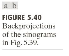
17 Examples: Laminogram 3/11/

18 The Fourier-Slice Theorem For a given value of θ, the 1-D Fourier transform of a projection with respect to ρ is j2πωρ Gw (, ) g(, ) e d θ = ρθ ρ j2πωρ G( ωθ, ) = f ( x, y) δ( x cosθ + y sin θ ρ) e dρdxdy = + = j2 f ( x, y) πωρ δ( x cosθ y sin θ ρ) e d ρ dxdy f ( x, y) e j2 πω ( xcosθ + ysin θ ) dxdy 3/11/

19 The Fourier-Slice Theorem j2πωρ Gw (, ) g(, ) e d θ = ρθ ρ j2 πω ( xcosθ + ysin θ ) G( ωθ, ) = f ( x, y) e dxdy j 2 π ( ux+ vy) = f ( x, y) e dxdy u= wcos θ, v= wsinθ = [ Fuv (, )] u= wcos θ, v= wsinθ = Fw ( cos θ, wsin θ) Fourier-slice theorem: The Fourier tansform of a projection is a slice of the 2-D Fourier transform of the region from which the projection was obtained 3/11/

20 Illustration of the Fourier-slice theorem 3/11/

21 Reconstruction Using Parallel-Beam Filtered Backprojections j 2 ( ux vy) f ( x, y) = π + F( u, v) e dudv Let u = wcos θ, v = w sin θ, then dudv = wdwdθ, 2π j2 πw( xcosθ+ ysin θ) f ( x, y) = F( wcos, wsin ) e wdwd 0 0 = θ θ θ 2π j2 πw( xcosθ+ ysin θ) G( w, θ) e wdwd 0 0 Gw (, θ ) = G( w, θ) π 2 ( cos sin ) (, ) (, ) j π f x y w G w e w x θ+ y θ = θ dwd 0 θ θ 3/11/

22 Reconstruction Using Parallel-Beam Filtered Backprojections π j2 πw( xcosθ+ ysin θ) f ( x, y) = w G( w, θ) e dwd 0 It s not integrable = π 0 (, θ) θ j2πwρ w G w e dw d ρ= xcosθ+ ysinθ θ Approach: Window the ramp so it becomes zero outside of a defined frequency interval. That is, a window band-limits the ramp filter. 3/11/

23 Hamming / Hann Widow 2π w c + ( c 1) cos 0 w ( M 1) hw ( ) = M 1 0 otherwise c c = 0.54, the function is called the Hamming window = 0.5, the function is called the Han window 3/11/

24 The Plot of Hamming Widow 3/11/

25 Filtered Backprojection The complete, filtered backprojection (to obtain the reconstructed image f(x,y) ) is described as follows: 1. Compute the 1-D Fourier transform of each projection 2. Multiply each Fourier transform by the filter function w which has been multiplied by a suitable (e.g., Hamming) window 3. Obtain the inverse 1-D Fourier transform of each resulting filtered transform 4. Integrate (sum) all the 1-D inverse transforms from step 3 3/11/

26 Examples: Filtered Backprojection 3/11/

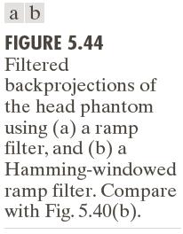
27 Examples: Filtered Backprojection 3/11/

28 Implementation of Filtered Backprojection in Spatial Domain Fourier transform of the product of two frequency domain functions is equal to the convolution of the spatial representation Let s(p) denote the inverse Fourier transform of w π j2πwρ f ( x, y) = w G( w, θ) e dw d 0 ρ= xcosθ+ ysinθ = π [ ( ) (, )] s ρ g ρθ dθ 0 ρ= xcosθ+ ysinθ π = g( ρθ, ) sx ( cosθ ysin θ ρ) dρ + dθ 0 θ 3/11/

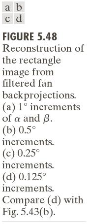
29 Reconstruction Using Fan-Beam Filtered Backprojections θ = α + β ρ = Dsinα 3/11/

30 Reconstruction Using Fan-Beam Filtered Backprojections Objects are encompassed within a circular area of radius T about the origin of the plane, or g( ρθ, )=0 for ρ >T π f( xy, ) = g( ρθ, ) sx ( cosθ ysin θ ρ) dρ + dθ 0 1 2π T = g( ρθ, ) sx ( cosθ + ysin θ ρ) dρdθ 2 0 T x= rcos ϕ; y = rsinϕ xcosθ + ysinθ = rcosϕcosθ + rsinϕsinθ = r cos( ϕ θ) 3/11/

31 Reconstruction Using Fan-Beam Filtered Backprojections x= rcos ϕ; y = rsinϕ xcosθ + ysinθ = rcosϕcosθ + rsinϕsinθ = r cos( ϕ θ) 1 2π T f( xy, ) = g( ρθ, ) sr [ cos( ϕ θ) ρ] dρdθ 2 0 T θ = α + β ρ = Dsin dρdθ = Dcosαdαdβ α 3/11/

32 Reconstruction Using Fan-Beam Filtered Backprojections dρdθ = Dcosαdαdβ 1 2π T f( xy, ) = (, ) [ cos( ) ] 2 0 gρθ sr ϕ θ ρ dρdθ T 1 1 2π α sin ( T/ D) = gd ( sin α, α β) sr 1 [ cos( α β ϕ) Dsinα] Dcosαdαdβ 2 α + + sin ( T/ D) 3/11/

33 Reconstruction Using Fan-Beam Filtered Backprojections 1 2π T f( xy, ) = (, ) [ cos( ) ] 2 0 gρθ sr ϕ θ ρ dρdθ T 1 1 2π α sin ( T/ D) = gd ( sin α, α β) sr 1 [ cos( α β ϕ) Dsinα] Dcosαdαdβ 2 α + + sin ( T/ D) 1 2π αm f( r, ϕ) = p( αβ, ) s Rsin ( α' α) Dcosαdαdβ 2 0 α m α sr ( sin α) = s( α) Rsinα 2 2π 1 αm f(, r ϕ) = q( αβ, ) h 2 ( α' α) dα dβ 0 R αm 2 1 α h( α) = s( α), q( αβ, ) = p( αβ, ) Dcosα 2 sinα 3/11/

34 3/11/

35 3/11/