Lecture 28: BLUP and Genomic Selection. Bruce Walsh lecture notes Synbreed course version 11 July 2013

Transcription

1 Lecture 28: BLUP and Genomic Selection Bruce Walsh lecture notes Synbreed course version 11 July

2 BLUP Selection The idea behind BLUP selection is very straightforward: An appropriate mixed-model is constructed (such as the animal model) to estimate individual breeding values These are called EBVs (estimated breeding values) or PBVs (predicted breeding values). The later because statisticians often speak of estimating fixed effects and predicting random effects. Individuals with the largest EBVs are chosen for the next generation The predicted response is simply the average of the EBVs in the selected parents. 2

3 Brief review: The general mixed model Vector of observations (phenotypes) Vector of fixed effects Incidence matrix for random effects Y = X! + Zu + e Vector of residual errors Incidence matrix for fixed effects Vector of random effects Observe y, X, Z. Estimate fixed effects! Predict random effects u, e 3

4 Henderson s Mixed Model Equations y = X! + Zu + e, u ~ (0,G), e ~ (0, R), cov(u,e) = 0, If X is n x p and Z is n x q p x p p x q XT R 1 X X T R 1 Z β = XT R 1 y Z T R 1 X Z T R 1 Z + G 1 û Z T R 1 y q x pq q x q The whole matrix is (p+q) x (p+q) Easier to numerically work with than BLUP/BLUE equations ( ) β = X T V 1 X 1 X T V 1 y ) û = GZ T V (y 1 X β V = ZGZ T + R Inversion of an n x n matrix 4

5 Matrix of PEV s 5

6 The Animal Model, y i = µ + a i + e i Here, the individual is the unit of analysis, with y i the phenotypic value of the individual and a i its BV 1 a 1 X = a 1.., β = µ, u = 2. G = σa 2 A, 1 a k Where the additive genetic relationship matrix A is given by A ij = 2" ij,,namely twice the coefficient of coancestry Assume R = # 2 e *I, so that R-1 = 1/(# 2 e )*I. Likewise, G = # 2 A *A, so that G-1 = 1/(# 2 A )*A-1. The animal model estimates the breeding value for each individual, even for a plant or tree! Same approach also works to estimate line (genotypic) values for inbreds. 6

7 The PEV and Accuracy Recall that the q x q submatrix C 22 in Has as its diagonal elements the Predictor error variances (PEV) for each EBV Hence, PEV ii = Var(EBV i - A i ), the variance of i-th predicted value breeding value around its true value. The smaller PEV ii, the more accurate the estimate of its BV. i s accuracy, $ i, is the correlation between the EBV and the true BV (recall accuracy of phenotype in predicting BV is h). 7

8 Reliability of EBVs The reliability of the EBV for individual i is just $ i2. Recalling that h 2 is the reliability of phenotype alone as a predictor of breeding value, the extent to which the reliability exceeds h 2 is a measure of how much information is added by relatives. PEV and $ are connected by PEV ii = (1- $ i2 )Var(A). Hence, can easily compute the reliability (and accuracy) for any EBV $ i 2 = 1 - PEV ii /Var(A). 8

9 Advantages of BLUP selection Easily accommodates fixed factors The relationship matrix A fully accounts for all different types of relatives Age-structure Drift Selection, assortative mating generated LD Unbalanced designs trivially handled Prediction of response (given EBVs of chosen parents) 9

10 Pitfalls of BLUP Strictly speaking, true BLUP assumes variance components are known without error Typically, use REML to estimate variances, and then use these in BLUP = empirical BLUP. This does not account for the error introduced into EBVs by error in the variance estimate. Using a fully Bayesian framework fully accommodates this concern. BLUP selection increases inbreeding relative to mass selection. 10

11 Extensions A number of extensions of the basic mixed model were examined in previous notes, e.g., repeated records common family effect genetic maternal effect associate effects The other major extension is multivariate BLUP, where a vector of traits is considered for each individual. The key for multivariate BLUP is that we form a single vector of random effects by simply stacking the individual vector of BVs for each trait. 11

12 For trait j (1 < j < k), the mixed model becomes We can write this as y = X! + Za+ e, where Again, the BLUP for the vector of all EBVs is given by ) â = GZ T V (y 1 - X β With V the covariance structure for this model 12

13 Covariance structure for EBVS The genetic variance-covariance matrix G accounts for the genetic covariances among traits. G has k variances and k(k-1)/2 covariances, which must be estimated (REML) from the data. 13

14 Covariance structure for residuals Here the matrix E accounts for within-individual correlations in the environmental (or residual) values. 14

15 Index selection Index selection with multivariate BLUPs is easy. If the merit function is H = % a i A i, then the BLUP of H for individual k is BLUP(H k ) = % a i *EBV(trait i for individual k) Note that since we are using estimated of breeding values, the index weights for the EBVs are the same as for the merit function. With phenotypic index selection, we were using phenotypic values, and hence the usual need for different weights on the selected index to maximize gain in the merit function (index of breeding values). 15

16 G-BLUP A key feature with BLUP is obtaining the relationship matrix A. This is typically done from the pedigree. However, pedigree-based A values are based on the expected relatedness between individuals, not their actual relationships. For example, 2" for full-sibs has an expected value of 1/2, but there is variation around this value, so that with two pairs of sibs, one may have a realized 2" of 0.38, the other Clearly, want to weight the second pair more, but using a pedigree-based A weights both sets equally (at 0.5). With sufficiently-dense genetic markers can actually estimate the realized value Using an A based on these genomic estimated of relationship is called G-BLUP (genomic BLUP), and A computed this way the genomic relationship matrix. 16

17 17

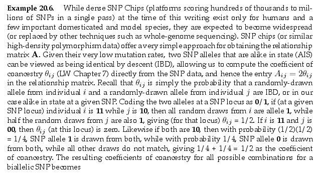
18 COC values for a given SNP 18

19 Genomic selection G-BLUP is an example of genomic selection, using very dense marker information to make inferences on breeding values. An extension of MAS, but now using very many markers (thousands +). Why do this? Predict BV in the absence of phenotype Such early-generation scoring can increase rate of response Improve estimate of BVs 19

20 EBVs for unmeasured individuals Before proceeding into genomic selection, we note that standard BLUP machinery allows us to estimate the breeding value of an unmeasured individual (i.e., an individual with no phenotypic record). GS also allows us to predict the breeding value for an unmeasured individual (no phenotype) for whom we also have genetic marker information. 20

21 Example Suppose individuals 1-3 are measured, 4 & 5 are not. Assume only a single fixed effect, the mean µ Model becomes 21

22 Here Letting Var(A) = 100, Var(e) = 100, V = ZGZ T + R = 200* I β = ( X T V 1 X) 1 X T V 1 y ) û = GZ T V (y 1 X β Gives BLUE(µ) = 11 returns Average base pop EBVs = 0 EBVs for individuals (4,5) with no phenotypic records Key: Information from relatives provides estimates for BV of unmeasured relatives. 22

23 Suppose we have maker data. How does this change EBVs? G-BLUP Suppose marker data gives A as 2 slightly inbred & 5 slightly less related than 1/2 sibs G-BLUP Pedigree-BLUP 23

24 Background issues for GS Before proceeding, some quick refreshers in QTL mapping and its limitations Linkage disequilibrium (LD) Association mapping The missing heritability problem 24

25 QTL mapping Marker-trait associations within a family, close pedigree, or (most powerfully) a line cross Relatively low marker density (~ 5-10 cm/marker) sufficient Relies on an excess of parental gametes to generate marker-trait association Widely used 1980 s ~ today, although ideas go back to 1917 and 1923 Power a function of differences in QTL allelic effects, marker-trait recombination frequency c Power for detection scales roughly as 2a(1-c) 2 Dependence of power on freq(q) is entirely through whether the sampled pedigree contains Q 25

26 Limitations of QTL mapping Poor resolution (~20 cm or greater in most designs with sample sizes in low to mid 100 s) Detected QTLs are thus large chromosomal regions Fine mapping requires either Further crosses (recombinations) involving regions of interest (i.e., RILs, NILs) Enormous sample sizes If marker-qtl distance is 0.5cM, require sample sizes in excess of 3400 to have a 95% chance of 10 (or more) recombination events in sample 10 recombination events allows one to separate effects that differ by ~ 0.6 SD 26

27 Limitations of QTL mapping (cont) Major QTLs typically fractionate QTLs of large effect (accounting for > 10% of the variance) are routinely discovered. However, a large QTL peak in an initial experiment generally becomes a series of smaller and smaller peaks upon subsequent fine-mapping. The Beavis effect: When power for detection is low, marker-trait associations declared to be statistically significant significantly overestimate their true effects. This effect can be very large (order of magnitude) when power is low. 27

28 Beavis Effect Also called the winner s curse in the GWAS literature Distribution of the realized value of an effect in a sample Significance threshold True value High power setting: Most realizations are to the right of the significance threshold, and the average value of these approaches the true value 28

29 In low power settings, most realizations are below the threshold, hence most of the time the effect is scored as being nonsignificant Significance threshold True value Mean among significant results However, the mean of those declared significant is much larger than the true mean 29

30 Background: LD: Linkage disequilibrium D(AB) = freq(ab) - freq(a)*freq(b). LD = 0 if A and B are independent. If LD not zero, correlation between A and B in the population If a marker and QTL are linked, then the marker and QTL alleles are in LD in close relatives, generating a marker-trait association. The decay of D: D(t) = (1-c) t D(0) here c is the recombination rate. Tightly-linked genes (small c) initially in LD can retain LD for long periods of time 30

31 Fine-mapping genes Suppose an allele causing an effect on the trait arose as a single mutation in a closed population New mutation arises on red chromosome Initially, the new mutation is largely associated with the red haplotype Hence, markers that define the red haplotype are likely to be associated (i.e. in LD) with the mutant allele 31

32 Background: Association mapping If one has a very large number of SNPs, then new mutations (such as those that influence a trait) will be in LD with very close SNPs for hundreds to thousands of generation, generating a marker-trait association. Association mapping looks over all sets of SNPs for trait- SNP associations. GWAS = genome-wide association studies. This is also the basis for genomic selection Main point from extensive human association studies Almost all QTLs have very small effects Marker-trait associations do not fully recapture all of the additive variance in the trait (due to incomplete LD) This has been called the missing heritability problem by human geneticists, but not really a problem at all (more shortly). 32

33 Association mapping Marker-trait associations within a population of unrelated individuals Very high marker density (~ 100s of markers/cm) required Marker density no less than the average track length of linkage disequilibrium (LD) Relies on very slow breakdown of initial LD generated by a new mutation near a marker to generate marker-trait associations LD decays very quickly unless very tight linkage Hence, resolution on the scale of LD in the population(s) being studied ( 1 ~ 40 kb) Widely used since mid 1990 s. Mainstay of human genetics, strong inroads in breeding, evolutionary genetics Power a function of the genetic variance of a QTL, not its mean effects 33

34 Association mapping (cont) Q/q is the polymorphic site contributing to trait variation, M/m alleles (at a SNP) used as a marker Let p be the frequency of M, and assume that Q only resides on the M background (complete disequilibrium) Haloptype QM qm qm Frequency rp (1-r)p 1-p effect a

35 Haloptype QM qm Frequency rp (1-r)p effect a 0 Effect of m = 0 Effect of M = ar qm 1-p 0 Genetic variation associated with Q = 2(rp)(1-rp)a 2 ~ 2rpa 2 when Q rare. Hence, little power if Q rare Genetic variation associated with marker M is 2p(1-p)(ar) 2 ~ 2pa 2 r 2 Ratio of marker/true effect variance is ~ r Hence, if Q rare within the A class, even less power, as M only captures a fraction of the associated QTL. 35

36 Common variants Association mapping is only powerful for common variants freq(q) moderate freq (r) of Q within M haplotypes modest to large Large effect alleles (a large) can leave small signals. The fraction of the actual variance accounted for by the markers is no greater than ~ ave(r), the average frequency of Q within a haplotype class Hence, don t expect to capture all of Var(A) with markers, esp. when QTL alleles are rare but markers are common (e.g. common SNPs, p > 0.05) Low power to detect G x G, G x E interactions 36

37 How wonderful that we have met with a paradox. Now we have some hope of making progress -- Neils Bohr Infamous figure from Nature on the angst of human geneticists over the finding that all of their discovered SNPs still accounted for only a fraction of relative-based heritability estimates of human disease. 37

38 The missing heritability pseudo paradox A number of GWAS workers noted that the sum of their significant marker variances was much less (typically 10%) than the additive variance estimated from biometrical methods The missing heritability problem was birthed from this observation. Not a paradox at all Low power means small effect (i.e. variance) sites are unlikely to be called as significant, esp. given the high stringency associated with control of false positives over tens of thousands of tests Further, even if all markers are detected, only a fraction ~ r (the frequency of the causative site within a marker haplotype class) of the underlying variance is accounted for. 38

39 From MAS to GS The idea behind MAS, which grew out of QTL mapping, was the thought that first QTLs could be detected, and then using marker tags, MAS selected on these QTLS to improve response Several problems QTLs really large chromosome regions ~ 40cM QTLs of large effect fractionate into smaller and smaller effects upon fine mapping Detected QTL effects are overestimated (Beavis effect) Human Association studies: most QTL of small effect Key paper: Meuwissen, Hayes & Goddard (2001) Skip trying to find QTLs altogether, use regressions involving ALL of the markers at once, use a training set to find the marker weights, and then use this to predict breeding values Problem of more marker genotypes than scored phenotypes (shrinkage methods, random models) 39

40 While today there is a huge and complex literature on genomic selection, all of the basic ideas were clearly defined in Meuwissen s et al, classic paper: Key concern: finding weights for all markers when number of markers >> number of scored (phenotyped) individuals. A lot of different approaches to do this have been proposed. Bottom line: GBLUP hard to beat, easy to do! 40

41 Genomic selection Meuwissen, Hayes & Goddard (MHG) noted that MAS does not work because the markers don t account for enough genetic variation Too few markers are used Markers used likely overestimate QTL effects (they were chosen because they had a significant effect) = Beavis effect Most QTLs likely have a very small effect Their solution: Include all of the markers into the analysis and then use statistical methods that shrink their effects. Random effects and Bayesian methods allow for number of markers to be >> than number of phenotypes scored Basic idea: Use a training set of individuals with marker information and high-quality estimates of breeding value to train a model (find regression parameters), then use this model to predict BVs of individuals with only marker info 41

42 WHG started with a simulated data set of ~ 50,000 markers in a population run for 1000 generations to reach mutation/drift equilibrium. Roughly ~ 2000 individuals where then phenotyped in generations 1001 and 1002 and used to train the model. ~2000 generation 1003 individuals were generated and their breeding values predicted using the model fit from gen 1001 & 1002 data The problem they faced was fitting ~ 50,000 marker effects with ~ 2000 data points (Breeding values) WHG s first model was standard least squares (LS) where each marker was tested separately, with those whose marker-trait effect exceeded a multiple-testing threshold chosen. The selected markers where then jointly fit in a multiple regression. GEBVs (genomic estimated breeding values) given by GEBVi = % k a k g i,k, where a k = weight in SNP marker k, g i,k = genotypic score at marker k for individual I. 42

43 Their three other models used a random-effects approach. Recall that under this framework, one estimates the variance of some underlying distribution from which individual realizations (here, the BV variance explained by a given SNP) then have their values predicted. This allows the ability to predict p >> n effects. Model one: BLUP. This assumes the SNP variance is the same for each marker (the expected variance is the same over all sites), so that a particular realization for a given marker is drawn from this distribution. Basically, this assumes the infinitesmal model, and is just GBLUP. Model two: BayesA. This assumes that QTLs at different SNPs may have a distribution of different values, so that for a given marker the expected value for the variance (which is used to generate the particular realization) is itself drawn from a distribution. MHG assumed this distribution for the expected variance at a marker was an inverse chi-square distribution, which has most effects small, but a few rare effects. 43

44 Model 3: BayesB. The problem with Bayes A is that all SNPs are assumed to have some nonzero marker variance (albeit very small). A potentially more realistic model is that a fraction & of sites have no variance, while the remainer (1- &) have their expected values drawn from some distribution, and (given this drawn value), a realization from for that site. Was computationally faster than Bayes A. Results: LS did very poorly, while the random effects models generally did well Benchmark: r ~ 0.4 for missing record with pedigree-blup, r ~ 0.8 for progeny test. 44

45 Different assumptions regarding the distribution of effects at the underlying (and unknown) QTLs leads to the many different models used for GS Hayes & Goddard Genome 53: 876 (2010) 45

46 Hayes & Goddard Genome 53: 876 (2010) A number of other methods, based on different assumptions around the distribution of QTL effects. A number are machine learning (semiparametric regression) approaches that make few assumptions about this underlying distribution, but are more in the form of taking a training set with some pattern (molecular data) with breeding values to generate some predictive function. Examples of such methods include support vector machines, semiparametric kernel regressions, and reproducing kernel Hilbert space regression. 46

47 Which version of GS to use? Different assumptions about these underlying distributions lead to different GEBVs estimators Generally, the differences are often small GBLUP is not only easy and robust, it is also often the best. Hence, recommendation is to use it unless only information suggests otherwise This is a model-fitting issue, as predictability of the model in the testing set provides some indication of which method is best. Hayes & Goddard suggest that if the aim of GS is to select across populations, that using a model assuming most SNPs have zero effect and just a few have moderate/large may be best, as this will located those QTLs segregating across lines/breeds 47

48 Accuracy improves with more records, closer marker spacing 48

49 Accuracy declines quickly over generations A closely-related issue is that a model trained (i.e., marker weights estimated) in one population does not translate to other populations. Models must also be retrained frequently. 49

50 Advantages of genomic selection (GS) While theoretically possible that genomic selection returns higher accuracies than standard phenotype/pedigree based BLUP EBVs, this is not typically while GS is used. Main use: speed up generation time Testing bulls in dairy cattle typically requires 6-7 years With GS, generation intervals down to 3 years Double rate of response, so if accuracy is at least half that of standard phenotype-based BLUP, increases the rate of response Concern is that the accuracy declines each generation This requires constant updating of the model and hence the constant updating of phenotypic records. 50

51 GS impact greatest for: Sex-limited traits Traits that are expensive to measure Traits measured only by destruction of an individual Traits expressed late in life Traits expressed after individuals are selected 51

52 GS and inbreeding Simulations show that GS is expected to reduce inbreeding per generation relative to standard BLUP. Reason is that it exploits the Mendelian segregation variance (two sibs equally weighted with pedigree BLUP, differentially weighted with genome-based weights), hence full sibs less likely to be co-selected. However, because of decreasing generation interval, rate of inbreeding/year may be larger. 52

53 How many SNPs needed? SNP density (number & spacing of makers) depends on the amount of LD in the population Rough rule: For accurate genomic breeding need LD between adjacent SNPs with r 2 > 0.2 The expected LD between two markers at recombination frequency c under mutation-drift is r 2 ~ 1/(4N e c + 1), or c ~ 1/Ne (for r 2 = 0.2) Meuwissen (2009) 10N e L markers need, where L = genome length For Holstein cattle, N e ~ 100, L = 30 Morgans (3000 cm), so that ~ 10*100*30 = 30,000 roughly equally-spaced SNPs Likewise, for N e = 100, c ~ 1/100 = 0.01 (for r 2 = 0.2). Number n of markers (given genomic length of 30 Morgans) again becomes ~ 30,

54 Accuracy of predicted values Hayes & Goodard show the accuracy of genomic prediction depends on the number q of independent chromosome segments in a population, with q ~ 2N e L N = number of phenotypic records in training population, h 2 = trait heritability This is first-generation of response. Accuracy declines in subsequent generations. 54

55 Hayes & Goddard Genome 53: 876 (2010) Assuming N e =