Internally generated preactivation of single neurons in human medial frontal cortex predicts volition

Transcription

1 Internally generated preactivation of single neurons in human medial frontal cortex predicts volition Itzhak Fried, Roy Mukamel, Gabriel Kreiman List of supplementary material Supplementary Tables (2) Supplementary Experimental Procedures Supplementary Figures (8) Supplementary Movie (1) 1

2 Table S1 (expanding on Table 1) PART A Temporal Lobe ACCr ACCd pre-sma SMA proper Total # of recorded cells Increase in rate ( I ) Decrease in rate ( D ) I + D Table S1, PART A: Anatomical distribution of units within the medial frontal lobe showing increase in firing rate ( I ) and decrease in firing rate ( D ) with respect to baseline. I + D indicates the sum of units showing I or D responses. SMA proper supplementary motor area proper; pre-sma pre-supplementary motor area, ACCd dorsal anterior cingulate cortex, ACCr rostral anterior cingulate cortex. See Figure S6 for MR images depicting electrode locations. 2

3 Table S1 (expanding on Table 1) PART B SUB ACCr ACCd SMA proper pre-sma TOTAL All MUA+SU A I D All MUA+SU A I D All MUA+SU A I D All MUA+SUA I D All MUA SUA I D Tot Table S1, PART B: Anatomical distribution of units within the medial frontal lobe in each subject. For each subject and location (see Part A for location abbreviations), we indicate the number of MUA units and SUA units and the number of units that showed an increase ( I ) or decrease ( D ) in firing rate as W was approached. 3

4 Table S2 (expanding on Table 1) Location A H EC ST PHG ACCr 8x10-5 2x10-5 4x10-6 8x10-5 2x10-5 ACCd 7x10-4 3x10-4 6x10-5 3x10-3 7x10-4 psma 9x10-4 3x10-4 5x10-5 4x10-3 9x10-4 SMA 5x10-9 9x x x10-8 5x10-9 Location ACCr ACCd psma SMA ACCr ACCd psma SMA 2x10-2 6x10-3 1x10-3 Comparison of the proportion of units that showed a statistically significant response before W among different areas using a binomial test. A significant response was defined by a ranksum test, p<0.01, 400 ms before W against baseline (Experimental Procedures). Let N 1, N 2 indicate the total number of units recorded from in area 1 and 2 respectively and let n 1, n 2 indicate the number of units that showed a significant response before W. f 1 =n 1 /N 1 and f 2 =n 2 /N 2 define the proportion of responsive units in each area. Under the null hypothesis, we assume that the two areas are indistinguishable and we compute the probability of obtaining n 1 or more responsive units (out of the total of N 1 units) assuming the proportion of responsive units in area 2 as p = N k =n 1 N 1 k (1 f 2 ) k f k 2. This table reports the p values for each pair of areas. Note that SMA has a significantly higher proportion of neurons responding before W compared to all other regions. The corresponding values of n 1, n 2, N 1, N 2 are reported in Table 1. 4

5 Supplementary Experimental Procedures EMG recordings We recorded electromyographic (EMG) signals in three healthy volunteer. We used EMG electrodes (Conmed Corporation, Billerica, MA) placed over the flexor digitorum sperficialis muscles. The data were recorded with the MicrguidePro system from Alpha Omega (Alpharetta, GA) with a 3 khz sampling rate and 500x amplification factor. The EMG data are shown in Figure S3C-D. Data analysis Classification of individual units. Baseline firing rate was defined as the spike count in the window from ms to ms relative to W (see also Figure S3E for other definitions of the baseline interval). We compared the firing rate during baseline with the firing rate in two different time windows using a non-parametric ranksum test and a threshold criterion of p < 0.01 (similar results were observed using a paired two-tailed t-test). The temporal windows were as follows: 1) 400 ms to 0 ms relative to W; 2) 0 ms to 400 ms following W. An analysis using a sliding window is presented in Figure 4. In Figure S1 we compared the changes in firing rate against those expected under three different null hypotheses (5000 iterations): (1) creating for each unit a surrogate spike train with the same firing rate as the actual unit but with the spike times governed by a homogeneous Poisson process (see also Figure 2C); (2) similar to (1) but here the surrogate spike train conserved not only the firing rate but also the interspike interval distribution of the actual spike trains and (3) randomly shifting W. We classified the response of all 128 units responding significantly before W (Table 1) as either showing increase in firing rate with respect to baseline ( I, n = 55) or decrease in firing rate with respect to baseline ( D, n = 73). To plot Figure 4A-C and S1G, the responses were normalized by subtracting the baseline activity and dividing by the maximum firing rate for I cells (or dividing by the absolute value of the minimum firing rate for D cells). After normalization, the responses were averaged. Statistical classifier. Figures 5-7 in the main text as well as Figures S4 use a Support Vector Machine (SVM) (Hung et al., 2005) classifier to quantify whether the neuronal ensemble showed changes in their firing patterns before W. The classifier yields a measure of performance at the single-trial level, as opposed to the typical Bereitschaftspotential averaged over a large number of repetitions (Colebatch, 2007; Erdler et al., 2000; Haggard and Eimer, 1999; Libet et al., 1983; Ohara et al., 2006; Yazawa et al., 2000). In Figures 5B, 5 and S4, we asked whether the classifier could discriminate the neuronal responses from baseline activity at a time t prior to W. Let represent the spike train for a given unit u on a given trial r ( τ i are the spike times). We binned the spikes in windows of size t r (the default value of t r =400 ms was 5

6 used throughout the text; the results were robust to changes in this parameter). Let indicate the spike count in a window of size t r centered at time t. For a population of n neurons, we assumed independent firing and we constructed a population vector by concatenating the responses of all units:. The number of units, n, depends on the specific analysis and is indicted in each figure legend. The baseline response was defined as c -2300, i.e., the spike count from to ms with respect to W. At any given time t, the input to the classifier consisted of the example vectors, r p t, containing the spike counts from the neuronal population for the training trials r associated with a label +1 and the baseline example vectors, r p -2300, associated with the label -1 (Figure S5A shows a simple example in the case of n=2 units). A binary classifier was trained to discriminate between the +1 and -1 examples, that is, to quantify whether the neuronal ensemble activity could be distinguished from baseline at a particular time and on a trial-by-trial basis. We used a linear kernel; in this case, the classifier boundary can be expressed as where the vector p denotes the ensemble response and the weights w are learnt during training. Other statistical classifiers and SVM kernels yielded similar results. The dimension of the input (the number of units n) is indicated for each figure in the text. We used a cross-validation procedure whereby we randomly chose 70% of the trials to be used for training and the remaining 30% of the trials were used to evaluate the classifier performance. This procedure was repeated in each one of 100 iterations. Importantly, the performance of the classifier was evaluated with independent data that was not seen by the classifier during training (i.e., there was no overlap between the training and test data). The performance of the classifier at time t indicates the percentage of test trials correctly discriminated from baseline at a time t prior to W. In those cases where we used a subset of the total number of units, we also randomly chose the units from the available population in each iteration. This was done, for example, in order to ensure that comparisons across areas were fair and not dictated by the higher number of recordings in one area. Error bars in the classifier performance plots denote one standard error and are based on this cross-validation procedure. Right versus left hemisphere. The decoding results discussed throughout the main text pool together units from both the right and left hemisphere. We also considered the performance of the classifier using separate neuronal subpopulations from either the right or left hemispheres in the task where subjects used only the right index finger (Figure 6D). We did not observe any significant difference in decoding performance between these two subpopulations. Single units versus multi-units. We divided the output spiking activity into multi-units (MUA, which cannot reliably be separated any further by the algorithm) and single-units (SUA) using the automatic criteria described in (Tankus et al., 2009). The plots in the main text and supplementary figures do not discriminate between SUA and MUA. We show the results obtained upon separating the SUA and MUA in Figure 6E. Essentially, both types of signals yielded similar results. 6

7 Prediction of W time. Figure 7 in the main text describes the performance of the classifier in predicting the time of volition onset (W). We bin the spike trains in windows of size t r (the default value of t r =400 ms was used throughout the text). Let indicate the spike count for unit u during trial r in a window of size t r centered at time t (Figure 7B). For a population of n neurons, we assumed independent firing and we constructed a population vector by concatenating the responses of all n units:. The time t was shifted in steps of 100 ms and therefore the spike count windows overlapped in time. For an ensemble of simultaneously recorded units, the spike trains were aligned to trial onset at t=0. When considering multiple recording sessions or multiple subjects, responses were aligned to W. Starting at t=-3500 ms, we constructed the vectors r p W-3500, r p W-3400,, r p W Each one of these vectors was associated with an indicator variable L(t) that labeled each window of size t r by +1 or -1 depending on the distance to W: L(t)=-1 if t<w-t b and L(t)=+1 if t W-t b. An SVM classifier was trained to learn the map between p and L (Hung et al., 2005). The performance of the classifier was tested using cross-validation by using new trials not seen by the classifier during training. The predicted urge/decision time,, was defined as the first time point when the classifier prediction on independent test data indicated L(t)=+1 in 3 out of 4 consecutive windows. Figure 7D in the main text shows the distribution of. Accuracy of W. Reporting W accurately is not trivial. Therefore, it is expected that there could be a variation between the reported W and the internal onset of the decision/urge to move. Unfortunately, it is not easy to estimate this variability (Joordens et al., 2002). We first reanalyzed all the data after assuming that W was reported in a random fashion. For this purpose, W was chosen randomly from a uniform distribution starting one clock revolution after trial onset and ending at P. This drastically reduced the number of significant units (Figure S1) and the classifier performance was close to chance levels. In order to further quantify the impact of changes in W time on the spiking responses and our analyses, we simulated inaccuracies in W by adding a fixed temporal bias (Figure S4D1) or random jitter (Figure S4D2) to W. This jitter was taken from a Gaussian distribution with zero mean and a standard deviation σ, with the constraint that W always had to occur before P. This analysis suggests that inaccuracies in W of several hundred ms would have led to a large decrease in the number of neurons responding before W. In particular, inaccuracies of several hundred ms would bring the results very close to chance levels. Yet, it is possible that there could be inaccuracy in W on the order of up to approximately 200 ms without impacting the overall number of significant neurons. Integrate-and-fire model. We speculate in the main text that the urge/decision may arise when a threshold is crossed after a cumulative increase in activity in the medial frontal lobe neuronal ensemble (Crick and Koch, 2003). Here we present a quantitative model of how this mechanism could work by using an integrate and fire model unit receiving input from the medial frontal lobe units recorded from in this study. The basic circuit for a leaky integrate-and-fire unit is shown in Figure S5G. The input current I(t) is integrated through an RC circuit: where C is the capacitance, R is the resistance and V is the voltage. When the voltage reaches a threshold V thres, a spike is generated, the voltage is reset to zero and a refractory period t ref is imposed. Each spike generated an EPSC and I(t) was modeled here as the 7

8 sum of all the input EPSCs. The parameters for the simulation shown in Figure S5H-I are given in the legend. Although the input to the model is given by the I units, it would be easy to also incorporate the D units by adding an additional sign change through an inhibitory interneuron. 8

9 Supplementary Movie 1 (related to Fig. 1): Activity of one neuron in left pre-sma during three trials of the task. Top panel depicts the analogue clock the patients observed. Bottom blue rasters and auditory beeps represent the occurrence of spikes. The black trace represents the spike train depicted by the blue rasters, smoothed with a Gaussian kernel (σ = 80ms). Red bar represents the time of button press and green bar represents the reported time of urge (W). List of Supplementary Figures Figure S1: Number of responsive units under the null hypotheses (related to Table 1). For each unit, we generated surrogate data by considering three possible null model hypotheses: (i) Poisson (green): We created a homogeneous Poisson spike train containing the same number of spikes as the real data. (ii) ISI (blue): We created a surrogate spike train that maintained the interspike interval distribution of the real data. (iii) Random W (red): We kept the original spike trains but the W time was generated randomly. We analyzed the surrogate data using the same methods and criteria applied to the real data (Experimental Procedures) and computed the number of responsive units (x-axis in A-F). A responsive unit was defined as a unit that showed a statistically significant change in firing rate when comparing the 400 ms pre-w and the to ms baseline period based on a ranksum test (p<0.01, Experimental Procedures). The procedure was repeated 5000 times. The plots show the distribution of the number of responsive units in the medial frontal lobe (A) and temporal lobe (B) for all units (A1,B1), I units (A2,B2) and D units (A3,B3). Subplots C-F show the corresponding distributions for the 4 different areas within the frontal lobe (ACCr = rostral anterior cingulate cortex; ACCd = dorsal anterior cingulate cortex; pre-sma = presupplementary motor area; SMA = supplementary motor area). The vertical dashed line shows the mean of the distribution and the dotted lines show 3 standard deviations from the mean. The arrow indicates the number of responsive units in the actual data. G1-G3. Control for Figure 4A based on surrogate data for the Poisson null model (G1), ISI null model (G2) and Random W null model (G3). The procedure to generate surrogate spike trains is described in A-F. Here we use the surrogate data to generate the equivalent to Figure 4A in the main text. The plot shows the normalized firing rate for the I cells (red) and the D cells (blue). Responsive cells were defined based on comparing the pre-w response period with the baseline period (shaded rectangles). For comparison, the dotted lines reproduce the normalized firing rate curves from Figure 4A. Note that the slight increase (decrease) in the red (blue) curve before W is restricted to the time window used in the statistical selection criteria (unlike Figure 4A where the deviations from baseline are more pronounced and start well before the selection window). FIGURE S2: Gradual versus abrupt transitions in single trials (related to Figs. 1-3) A. Schematic example of a hypothetical unit that shows gradual changes in activity in individual trials leading to an gradual increase in firing rate in the average PSTH (right, average of 100 trials). 9

10 B. Schematic example of a hypothetical unit that shows abrupt changes in activity with variable transition times in individual trials leading to a gradual increase in firing rate in the average PSTH (right, average of 100 trials). C. To quantify the degree to which transitions in individual trials should be described as abrupt versus gradual, we considered the spike trains from individual trials in the 2500 ms preceding W after smoothing with a 200 ms width Gaussian. We fit a logistic function, f f (t) = W 1+ exp[ (t t 0 ) / α] + f, (where f B W and f B are the firing rates before W and during the baseline respectively, and t 0, α are free parameters to be fitted. Here we show the shape of the logistic function for different values of α showing abrupt changes (low values of α) or gradual changes (large values of α). D-E. Examples of individual trials (different units) showing the smoothed spike train (blue) and the logistic function fit (red). Note that the function was fit only in the 2500 ms preceding W. In each example, we show the value of α and the Pearson correlation coefficient between the fitted function and the smoothed spike train. The three examples in D show α values larger than the mean (more gradual transitions) whereas the three examples in E show α values smaller than the mean (more abrupt transitions). F. Distribution of fitted α values for n=55 units that showed increases in firing rate as W was approached (Table S1A). The dashed line and the dotted lines show the mean and SD of the distribution respectively. Note the logarithmic scale on the x-axis. G. Distribution of fitted t 0 values for the same n=55 units. H. Distribution of Pearson correlation coefficient (r) between the fitted logistic function and the smoothed spike train. We only considered those trials that yielded r>0.5 for the distributions in F-H. Figure S3: EMG, baseline and neuronal response dynamics (related to Fig. 1-3) A. Fraction of trials where P occurred within x milliseconds after the first revolution of the clock (where x is the value indicated in the x-axis). When x is very short, these trials could be considered to be cued trials where the end of the first revolution of the clock is the cue. As the plot shows, there were very few trials with P<1000 ms after the first revolution of the clock. Error bars indicate the range across all subjects. B. For the 6 responsive units where we had at least 10 repetitions with P < 1500 ms after the first revolution of the clock, we show the PSTHs aligned to W (t=0) for those trials with P<1500 ms (blue), those trials with P>5000 ms (red) and all trials (black). The numbers at the bottom of each subplot indicate the number of trials for each condition. We also indicate the location of each unit at the bottom of each subplot (see Table 1 for abbreviations). C. Example average EMG recordings from one session and one subject. We recorded EMG signals in three subjects (see Experimental Procedures for methods and EMG electrode locations). We note that we did not perform neurophysiological recordings in these three subjects. Here we show the EMG signals aligned to the key press events (t=0) and averaged across all trials (n=158). The gray lines denote one SEM. 10

11 D. Distribution of EMG to Key-Press latencies. In each trial, we computed the first time point when the EMG signal deviated from baseline by more than 5 standard deviations. This time point was defined at the EMG onset. Here we show the distribution of EMG onset to Key Press latencies across all three subjects and all recording sessions. Bin size = 5 ms. The vertical dashed line denotes the mean. E. Fraction of responsive units as a function of the time to W for different definitions of the baseline period (shaded rectangle): E1: to ms; E2: to ms; E3: to ms; E4: to ms (this is the baseline used throughout the text). A unit was considered to be responsive if the firing rate in the 400 ms centered on the time point reported on the x-axis was significantly different from the firing rate in the baseline period (two sided t test, p<0.05). The fraction of responsive units at each time point was computed by dividing the number of responsive units by the maximum number of responsive units across all baselines and time points (filled circle in E3). We indicate the average number of trials for each possible baseline definition. In E4, we point to the baseline and time point used in the numbers reported in the text and in Table 1. F. Comparison among trials when P-W<300 ms (blue), trials when P-W>600 ms (red) and all trials (black). Each subplot shows the PSTH for a separate unit aligned to W (left) or P (right). The format for the PSTHs is the same as in Figure 3 in the main text. The vertical lines indicate the mean W times (left) or mean P times (right); the color code for the means matches the one for the corresponding curves. The number of trials in each condition is indicated at the bottom of each subplot. G. Average normalized PSTH aligned to W (left) or P (right) for all the responsive I units (n=6) that had at least 5 trials with P-W>600 ms. Figure S4: Neuronal response onset correlates with W and P. Estimating the effect of inaccuracies in W (related to Fig.1-4). A. Example trial illustrating the definition of response onset in a single trial. Defining response onsets in single trials is not easy due to the intrinsic variability in neuronal firing. We used the following heuristic to define the response onsets. At each time point, t (step size = 40 ms), we defined fr(t) as the spike count in the time interval from t to t+400 ms and (that is, λ(t) takes the value +1 if the spike count increased in the last 40 ms and -1 otherwise). We considered a window w of 15 consecutive bins and we defined a score. The response onset was defined as the first time point where S 8. This time point is indicated by the blue vertical dashed line in this figure. The conclusions from this figure were not changed when we used different parameters to define the response onset. B. Three example units showing W versus response onset. Each circle corresponds to a separate trial. The black diagonal represents the identity line. The blue dashed line indicates the linear fit. For each responsive unit, we computed a correlation coefficient between W and the response onset and between P and response onset. The red dashed line indicates the time of first clock revolution. C. Distribution of correlation coefficients between W and response onset (C1) and between P and response onset (C2). Bin size = 0.1. The arrow indicates the mean of the distribution. There is no significant difference between these correlation coefficients for W and P. 11

12 D. We estimated the effect of inaccuracies in the W judgment. We simulated two types of inaccuracies: temporal shifts (D1) and random temporal jitter (D2). The effects were evaluated by computing the number of units that passed the same statistical criteria to be considered responsive and normalizing the results by the values reported in the text (which correspond to no temporal shift or temporal jitter). D1. The time of W was shifted by the amount indicated in the x-axis. Negative values indicate shifting to earlier time points and positive values indicate shifting to later time points. In each trial the maximum allowed positive shift was bounded by P. Because P was typically close to W (P- W=193±261 ms, mean±s.d. Figure 1) there are few points after shift=0 ms. The arrow shows the maximum number of significant units, which was obtained for a temporal shift of -50 ms. The red circles correspond to I cells (cells that increase their firing rate as W approaches), the blue circles correspond to D cells (cells that decrease their firing rate as W approaches) and the black circles include both I and D cells. D2. In each trial, the time of W was randomly jittered by adding or subtracting a time taken from a zero-mean Gaussian distribution and standard deviation σ (x-axis). The jitter was constrained to be such that W<P and that W was larger than the first revolution of the clock. After randomly jittering W in each trial, we repeated the same analysis to assess whether each unit shows significant pre-w response with respect to baseline. Here we show the fraction of units that show significance with respect to the σ=0 (no jitter) condition. The red circles correspond to I cells, the blue circles correspond to D cells and the black circles include both I and D cells. Inaccuracies in reporting W on the order of ~ 0 to 200 ms yield only a small decrease in the percentage of responsive units suggesting that subjects reported W with an accuracy of a few hundred ms. Results shown correspond to the mean±sd after 1000 iterations (to avoid clutter, error bars are shown only for the black circles). The horizontal dashed line corresponds to chance levels obtained by repeating the same analysis using surrogate spike trains (corresponding to the green curves in Figure S1). Figure S5: Decoding self-initiated movement in single trials and integrate-and-fire model (related to Fig. 5-6) A. Simplified version of the classifier task for n=2 units to illustrate the algorithm to decode volition in single trials. Responses of two units located in the pre-sma during the 400 ms before W (circles) or during the baseline interval from to ms (crosses). Many of the points overlap due to obtaining the same spike count in different repetitions; therefore, a single point in the figure may correspond to multiple repetitions. Also, the number of spikes for the circles and crosses could overlap; to avoid this and only for the purposes of the figure (not for the classifier) we added here a value of 0.2 to the circles and we subtracted 0.2 from the crosses. A fraction of the data on the left (70% of the repetitions) is used to train a linear classifier to learn to separate the circles and crosses (i.e., to separate the spike counts in the interval before W and baseline interval) by finding an appropriate hyperplane (a line in the 2D case with a linear classifier). On the right we show the same data and the classifier boundary (dashed line). The output of the classifier is indicated by the color of the symbols, red corresponds to circle predictions and blue corresponds to cross predictions. The overall performance of the classifier is given by the fraction of repetitions in the remaining 30% of test data that are correctly classified (red circles and blue crosses). In most of the figures in the main text, the procedure was applied to ensembles of many more than 2 units (see main text and Experimental Procedures for details). 12

13 B. Dependence of the classification performance on the size of the spike count window (referred to as t r in Experimental Procedures). The value highlighted in gray corresponds to the parameter used throughout the text. Here the classification performance is shown at two time points: 500 ms (green) and 1000 ms (red) before W. Error bars denote SEM. C. Classification performance for each individual subject and each location. The thin lines represent individual subjects and the thick line shows the average across all subjects in each location. In each subplot, we only included those subjects with at least 16 units in the corresponding location. D. Classification performance for each subject that had at least 16 units in the frontal lobe. Here we show the classification performance in the [-400,0] ms window. The error bars denote one standard deviation over randomizations of the units and repetitions (see text). The horizontal dashed line and its error bar on the right indicate the mean and range of the chance classification performance obtained by a permutation test (see text). Note that except for subject number 4, the classification performance was well above chance using data from individual subjects. Table S1B also describes the number of units recorded from in each subject and location as well as the number of units that showed significant responses for each individual subject and location. There is a significant amount of subject-to-subject variability. At least partly, these differences can be attributed to different number of electrodes and different recording locations across subjects. E. Decoding accuracy as a function of time to W using classifiers trained with different numbers of units. Spikes were counted in windows of 400 ms centered on the time point indicated on the x-axis. The time on the x-axis is measured with respect to W (dashed vertical line at t=0). Figure 6A in the main text reports the counterpart to this figure where we showed the performance of the classifier at two specific times as a function of the number of units. Here we show the time course of the decoding performance. Overall, it is remarkable that a minuscule fraction of the total number of neurons in the frontal lobe areas is sufficient to achieve strong classifier performance, and that even within this small group, decoding performance improves with the number of neurons used (Figure 6A). It is not unreasonable to expect that a decoder using more neurons could perform at even higher levels and perhaps even make more sophisticated behavioral predictions. However, we should note that the use of a SVM classifier here does not imply that the brain decodes the onset of volition using similar algorithms or classifiers (see also Figure S5). F. Classification performance separated by location (average across subjects). For each location (ACCr=green, ACCd=black, pre-sma=red, SMA=blue), we consider here only those subjects where we had at least 16 units. The numbers next to each curve indicate the number of subjects. The error bars denote one standard deviation across subjects. The horizontal dashed line indicates chance performance and the vertical dashed line denotes W. G. Schematic diagram of a basic model to illustrate how a leaky integration followed by a threshold mechanism could lead to the volitional onset. The input to the integrate-and-fire model here corresponds to the spiking activity of the units recorded from the human frontal lobe (shown schematically on the left). Each spike generates an EPSC and the input current to the model unit is the sum of all the input EPSCs. The leaky integrator fires a spike whenever the voltage crosses a threshold, and then resets the voltage back to zero. A refractory period is imposed 13

14 after each spike. Both excitatory and inhibitory units are used here as input (a minus sign is added to the synaptic weight for the inhibitory units). H. Distribution of the spike times for the I&F model with respect to the W time (n=40 trials). Bin size = 100 ms. The arrow indicates the mean of the distribution. I. Integrate-and-fire model (I&F) performance. Here we show the performance of the integrate and fire model illustrated in part A (parameters: C=32, R=256, α=0.01, v thres =1.6) during 2 trials (out of the 40 trials used to run the simulation). The first column shows the input to the model, consisting of the spikes of the frontal lobe units, including both excitatory and inhibitory ones. The green dashed line indicates W. The second column shows the activity of each unit during the 10 ms preceding a spike in the I&F model. Each row corresponds to a medial frontal cortex unit, each column corresponds to a 1 ms bin and the white marks denote a spike. The third column indicates the EPSCs, the input to the I&F, immediately preceding a spike. The fourth column shows the evolution of the intracellular voltage in the I&F unit as a function of time. The vertical green dashed line at t=0 indicates the W time. The horizontal dashed line shows the threshold for the I&F model, a spike (vertical black dashed line) is emitted when the voltage reaches this threshold. The number to the right in each trial indicates the time of the I&F spike relative to W. Figure S6. Anatomical location of electrodes in the frontal lobe displayed on individual MR images for each subject (related to Table 1). Color code: blue = SMA proper, red = pre-sma, yellow = ACCd, green = ACCr. Figure S7: Hand choice experiment (related to Figures 2-4). Three subjects performed a variant of the main experiment where they were allowed to choose not only the time of action but also which hand to use. A-C. Here we show examples of single unit responses during this variant of the task. The format is similar to the one in Figure 3. The plots show the raster plots and firing rates as a function of the time to W (t=0). The red traces (blue traces) show the average response when the subject executed the movement with the right hand (left hand). Above each subplot, an * indicates whether a two-tailed t-test between the blue and red curves was significant at the p<0.05 level in each time bin. We indicate the location of the electrode in each subplot. A1-A3 show examples of units that showed gradual changes in firing rate that were largely independent of the hand choice. B1-B3 show examples of units that showed enhanced activity when the subject opted to use his right hand. C1-C3 show examples of units that showed enhanced activity when the subject opted to use his left hand. The sharp drop in firing rate after W in C3 constitutes an edge effect artifact. The rightmost column (A4,B4,C4) shows the normalized firing rate for each of the three types of responses illustrated in A-C (the format is similar to the one in Figure 4A). The number of units averaged was 6 (A4), 6 (B4) and 4 (C4). D. The pre-w activity of the neuronal ensemble can extrapolate across hands. Here we show the performance of the classifier in one subject (36 units) that was allowed to freely choose which hand to use to perform the movement (in addition to choosing the time of action). The format is similar to the one in Figure 5B. In the blue curve, we trained the classifier using the ensemble responses from those trials where the 14

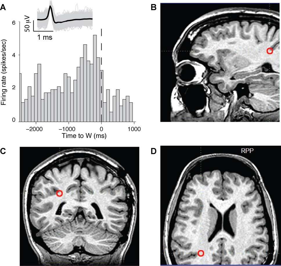
15 subject opted to use his right hand and tested the classification performance using the responses from those trials when the subject opted to use his left hand. In the red curve, we trained the classifier using the left hand trials and tested its performance on the right hand trials. E. The pre-w activity of the neuronal ensemble also allows us to predict which hand the subject will opt to use. Here the classifier was trained to predict the hand choice (blue curve). The black points indicate the performance obtained upon randomly shuffling the right hand / left hand labels. Figure S8: Recordings from parietal cortex. We recorded the activity of units in the right posterior parietal cortex in one additional subject. The unit illustrated in A showed a gradual increase in firing rate as W was approached. There were 3 units that showed this effect in the right posterior parietal cortex (out of a total of 13 recorded units). The MR images in B-D depict the electrode s location (red circle). 15

16 Figure S1

17 FIGURE S2

18 Figure S3

19 Figure S4

20 Figure S5

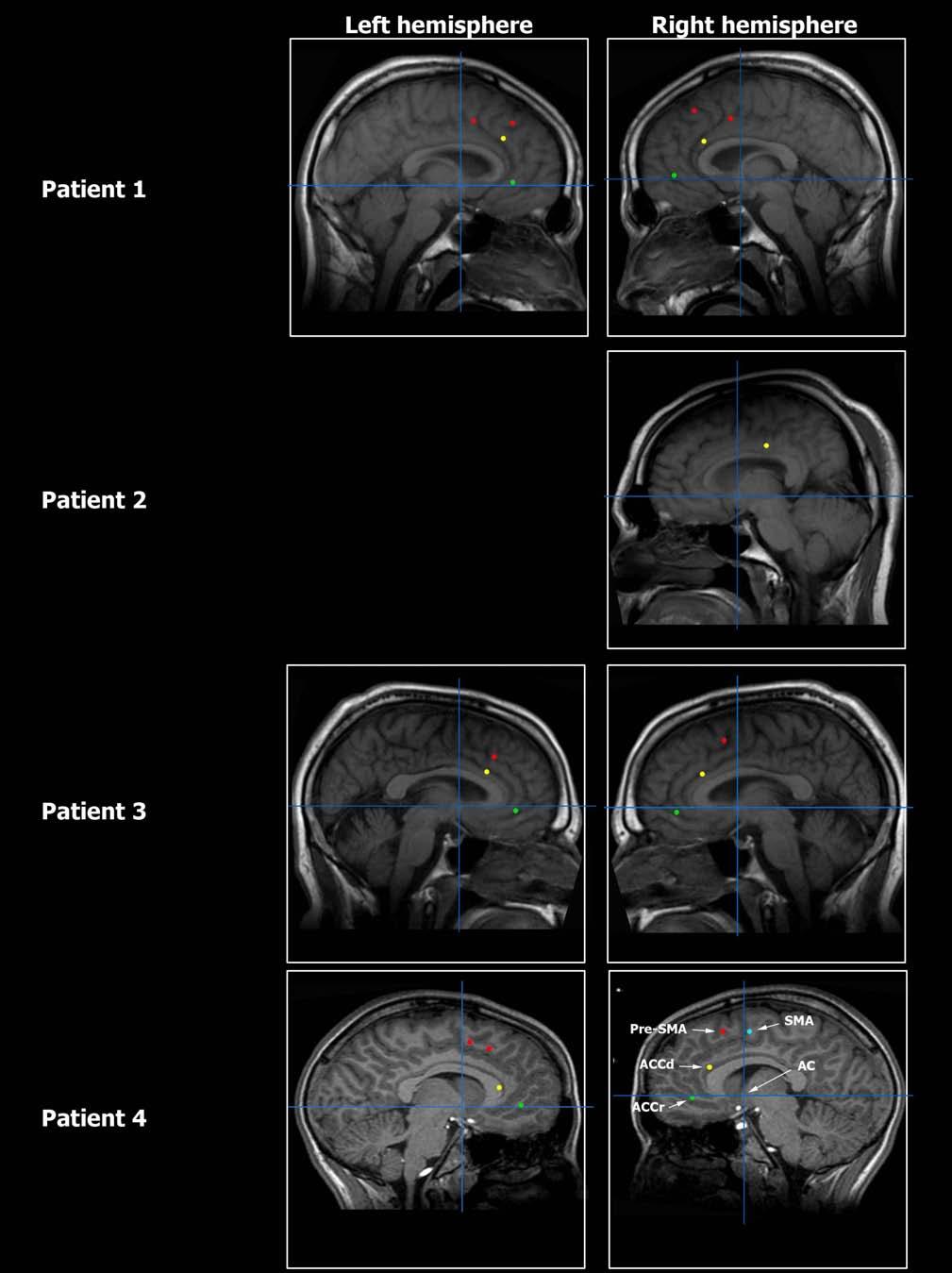
21 Figure S6

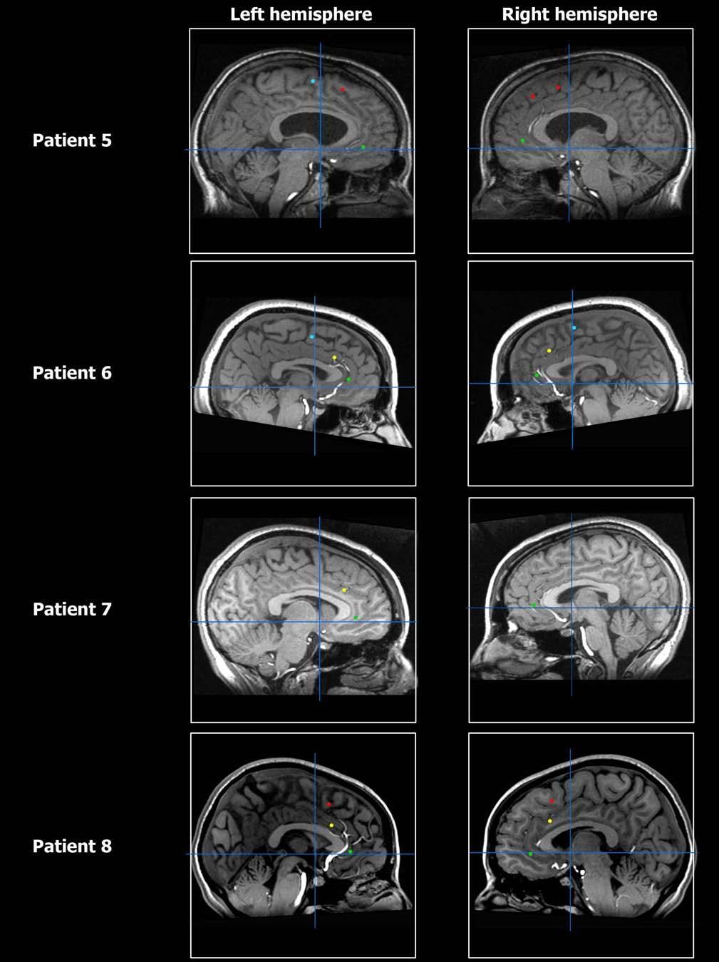
22 Figure S6

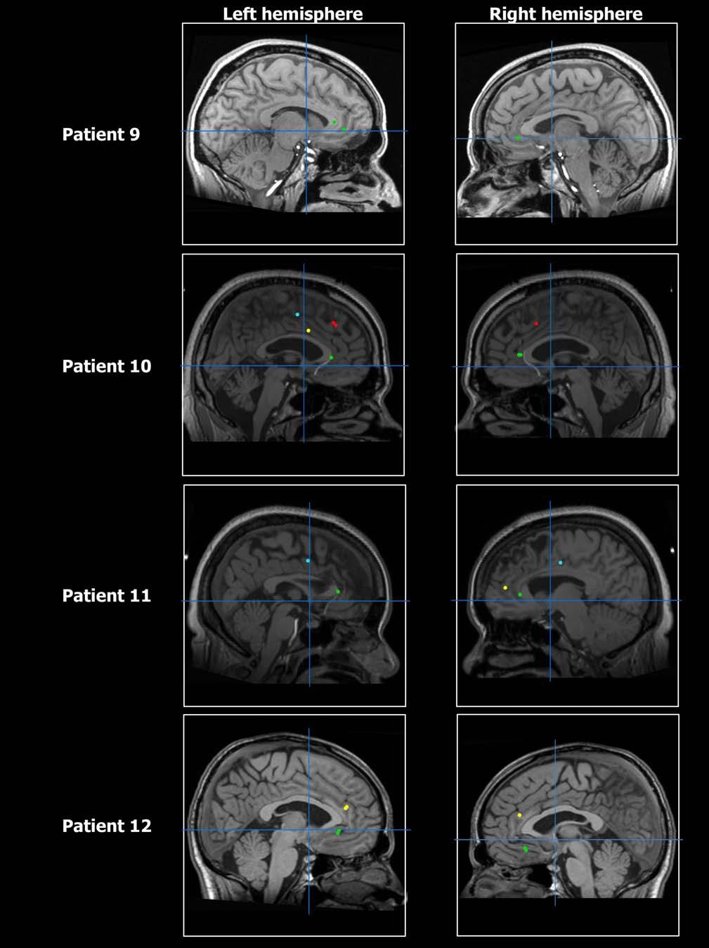
23 Figure S6

24 Figure S7

25 Figure S8