Every animal is represented by a blue circle. Correlation was measured by Spearman s rank correlation coefficient (ρ).

Transcription

1 Supplementary Figure 1 Correlations between tone and context freezing by animal in each of the four groups in experiment 1. Every animal is represented by a blue circle. Correlation was measured by Spearman s rank correlation coefficient (ρ).

2 Supplementary Figure 2 Comparisons of context memory between groups are stable over time and invariant to the salience of the conditioning context.

3 (a) Minute-by-minute analysis of freezing during the context test for the groups in experiment 1 (and Pairings Last, included for illustration but not in the statistical analysis). A repeated measures ANOVA showed no Time*Contingency*Spacing interaction (n = 16,17,18,20,21,F 1,288 = 1.96, P = 0.17). A comparison restricted to the massed condition (between CTL II and Pairings First) also showed no Time*Contingency interaction (F 1, 144 ) = 0.74, P =0.40). (b) Comparison of CTL II and Pairings First groups with conditioning and context test performed in a more salient context (lit by a visible light and with citrus odor). Reduction in Tone memory matched previous result (ratio between CTLII and Pairings First 0.63 vs originally), whereas Context memory was similar between the groups, as before. Error bars indicate s.e.m.

4 Supplementary Figure 3 Defecation gives similar results to freezing for experiments described in Figure 2. (a) Contingency degradation in the Intermixed condition with APV infusion in dorsal hippocampus (DH) prior to conditioning, as measured by defecation during tone test. (n = 9,9, Mann-Whitney U test, U = 17.5, P = 0.04). (b) Impaired contextual aversive memory, as measured by defecation, following APV infusion in DH prior to conditioning (n = 9,7, Mann-Whitney U test, U = 9.5, P = 0.018). Error bars indicate s.e.m.

5

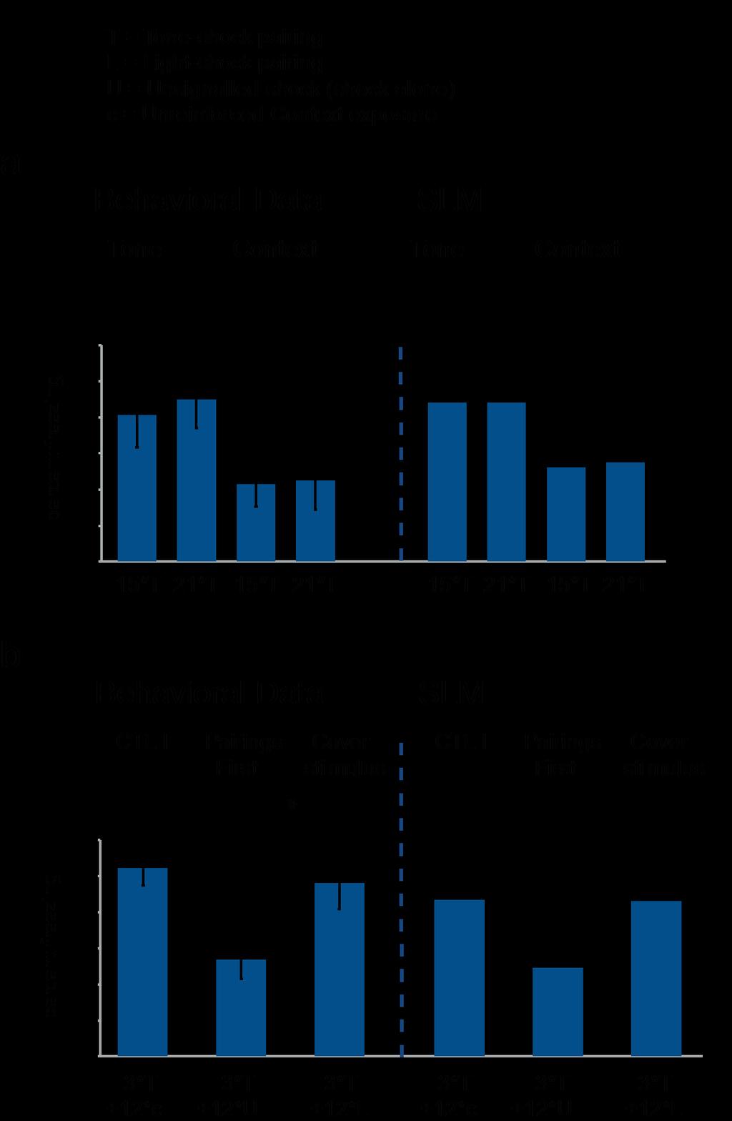
6 Supplementary Figure 4 Effect of repeated USs depends on contingencies. (a) Behavioral data (left) and model simulation (right) for conditioning with 15, and 21 CS-US pairings (n=9, 7). Adding further shocks paired with the same tone CS (21 pairings in total) did not reduce tone memory strength. (b) Behavioral data (left) and model simulation (right) for the cover stimulus effect. Signaling shocks with a second CS (in this case a flashing light), instead of giving unsignaled shocks attenuates contingency degradation (comparison between Pairings First and Cover Stimulus groups, n = 18, 12, unpaired sample t-test, t 28 = 2.42, * P = 0.022) Error bars indicate s.e.m.

7 Supplementary Figure 5 Location of the optical fiber tips for optogenetic experiments.

8

9 Supplementary Figure 6 Location of the electrode tips for electrophysiological experiments.

10 Supplementary Figure 7 Effects of contingency on amygdala LFP potentiation. (a) Example traces before, and after conditioning for a representative animal each in the Control II group (left) and Pairings First group (right). Red arrows indicate the peak depolarization. (b) Averaged peak depolarizations in the CTL II and Pairings First groups before (Habituation), and after (LTM) conditioning. There was a marginally significant interaction between time and contingency (n=10, 8, repeated measures ANOVA, F = 1, , P=0.055), and a simple effects analysis showed significant potentiation of the LFP response in the CTL II, but not the Pairings First condition (F = 18.0, P = and F 1,16 1,16 = 1.022, P = 0.33), further indicating that conditioning differentially effects synaptic processing depending on contingency. Error bars indicate s.e.m.

11 I II mixed First Supplementary Figure 8 Comparison of SLM to behavioral results for experiments described in Figure 1. Direct comparison of behavioral data (top panel) and SLM (bottom panel) for experiment 1. Error bars indicate s.e.m.

12 Supplementary Figure 9 The graph structures used for SLM, extended to include a second discrete variable.

13

14 Supplementary Figure 10 SLM s predictions for further conditioning phenomena. (a) Cover stimulus effect: Replacing unsignaled USs by USs signaled by a second discrete cue (e.g. a light) reverses the effects of contingency degradation. (b) Overshadowing: Conditioning to a single cue (Tone) is reduced if it is trained in compound with a second cue (Light). (c) Recovery from overshadowing: Unreinforced presentations of the overshadowing second cue (Light) restores the level of responding to the first cue. (d) Blocking: Initial conditioning to a Light reduces subsequent conditioning to the Tone when the Tone is conditioned in compound with the Light.

15 Supplementary Figure 11 Graphical illustration of the fits of some of the different models compared. (a) Behavioral Data. (b) Bayesian model that learned both structure and parameters (SPLM). (c) Bayesian model that learned parameters using Graph 6 (from Fig. 5a) and the best Beta priors for edge parameters. (d) Van Hamme and Wasserman s extension of the Rescorla-Wagner model.

16 Model MSE s.e. of MSE for hippoampus the MSE APV injection (% freezing squared) Parameters Structure Learning (SLM) Parameter Learning (PLM) SLM no Background PLM no Background SLM Linear SOCR with Background HW-RW with Background SOCR HW-RW Supplementary Table 1: Comparison of model fits. Mean squared error (MSE) for the best fit of each model, followed by the standard error of the MSE, and the error of the model in predicting the results of hippocampal interventions, with each value representing percentage freezing squared. The final column lists the number of free parameters (excluding the two scaling parameters). Model BIC Adjusted R 2 Adjusted R 2 Context Tone SLM SLM no Background SLM linear SPLM PLM SOCR HW-RW Supplementary Table 2: Bayesian Information Criterion (BIC) and adjusted R-squared values for the different models. For BIC the number of data points was 29, and the number of parameters was the number of model parameters plus the two scaling parameters. R-squared values were adjusted by the number of model parameters plus 1 scaling parameter.

17 Training protocol 2*U 3*U 6*U 10*U 15*U 2*U +1*E 3*U+1*E n= Training protocol 2*P 3*P 6*P 10*P 15*P 21*P n= including with CS test only Training protocol 3*P+3*U 3*P+6*U 3*P+9*U 3*P+12*U Intermixed 12*U+3*P n= including with CS test only Supplementary Table 3: Group sizes for the different conditioning protocols. Experiment 1 Tone Context F statistic p value F statistic p value Interaction F 1,71 = F 1,71 = Main effect for test order F 1,71 = F 1,71 = All experiments with varied test order Tone Context F statistic p value F statistic p value Interaction F 1,116 = F 1,116 = Main effect for test order F 1,116 = F 1,116 = Supplementary Table 4: The order of the CS and Context tests didn t significantly affect freezing scores either for the groups in Experiment 1, or across all the different conditioning protocols where the order of the testing was varied. Testing order was varied for all protocols except when only CS-US pairings were given. For those, the context test was always given first to get the best possible measure of the overshadowing effect. Analysis using Two-way ANOVA, with the levels of the first factor being the different conditioning protocols.

18 Group Latency HAB Latency LTM Amplitude HAB Amplitude LTM as % from HAB (ms) (µv) (µv) Control II ± ± ± ± Pairings First ± ± ± ± Supplementary Table 5: There was no statistically significant effect of group or conditioning on A-LFP latencies (p values for main effects and interaction > 0.7), or between average amplitudes during habituation between groups (p > 0.4). However, the increase (as percentage baseline) in A-LFP amplitude amplitude following conditioning was significantly higher in the 100% contingency group Control II (p = 0.028).

19 Experiment 1-no manipulation Tone Context F statistic p value F statistic p value Interaction F 1,75 = F 1,75 = Main effect for contingency F 1,75 = F 1,75 = Main effect for spacing of CS-US pairings F 1,75 = F 1,75 = Simple main effect for contingency with pairings spaced F 1,75 = F 1,75 = Simple main effect for contingency with pairings massed F 1,75 = F 1,75 = Simple main effect for spacing with 100% contingency F 1,75 = F 1,75 = Simple main effect for spacing with 20% contingency F 1,75 = F 1,75 = Experiment 2-APV infusions (Fig. 2b,c) Tone Context F statistic p value F statistic p value Interaction F 1,32 = F 1,32 = Main effect for contingency F 1,32 = F 1,32 = Main effect for drug F 1,32 = F 1,32 = Experiment 2-APV infusions (Fig. 2d,e) Tone Context t statistic p value t statistic p value t 16 = t 14 = Experiment 3-optogenetic inactivation Tone Context F statistic p value F statistic p value Interaction F 1,29 = F 1,29 = Main effect for laser treatment F 1,29 = F 1,29 = Main effect for spacing of CS-US pairings F 1,29 = F 1,29 = Simple main effect for laser with pairings spaced F 1,29 = F 1,29 = Simple main effect for laser with pairings massed F 1,29 = F 1,29 = Experiment 4 LFP potentiation Tone t statistic p value t statistic p value t 11.1 = t 11.0 = Supplementary Table 6: F and p values from Two-way ANOVA comparisons for Experiments 1-3 and t statistics for Experiments 2 and 4.

20 Experiment 1-no manipulation Tone Context % freezing CTL I ± ± 0.91 CTLII ± ± 5.50 Intermixed ± ± 6.06 Pairings First ± ± 5.94 Experiment 2-APV infusions Tone Context % freezing Vehicle CTLII ± ± 5.87 Vehicle Pairings First 18.2 ± ± 2.31 APV CTL II ± ± APV Pairings First ± ± 0.29 Vehicle Intermixed ± 9.57 (Defecation ± 1.23) APV CTL I ± 9.62 (Defecation 6.88 ± 0.73) APV Intermixed ± ± 0.22 (Defecation 3.89 ± ± 0.70) Experiment 3-optogenetic inactivation Tone Context % freezing Pairings First/Laser Offset ± ± 9.38 Pairings Firs/Laser Overlap ± ± 8.05 Intermixed/LaserOffset ± ± 6.99 Intermixed/Laser Overlap 35.1 ± ± 8.61 Experiment 4-Electrophysiology Tone % freezing Control II ± Pairings Firs 9.87 ± 2.66 Cover Stimulus ± 7.15 Supplementary Table 7: Mean ± standard error freezing (and defecation) scores.

21 Structure learning model Structure & parameter learning model Parameter learning model Extended Comparator Hypothesis Extended Rescorla- Wagner model α = a 1 = a 1 = s 1 = T a 1 = ρ = b 1 = b 1 = s 2 = T a 2 = a 2 = a 2 = s 3 = T b 1 = b 2 = b 2 = k 1 = 0.05 T b 2 = a 3 = a 3 = k 2 = Ca 1 = b 3 = b 3 = k 3 = 1.00 Ca 2 = a 4 = a 4 = Cb 1 = b 4 = b 4 = Cb 2 = ρ = Supplementary Table 8: Best fit parameters for Bayesian and Associative models.

22 Supplementary Modeling Stationarity Our Bayesian models assume that trials come from a stationary process and therefore ignore trial order effects. This is a good match for our data where we only see weak ordering effects, and is a suitable strategy for learning the structure of the environment, since the presence or absence of a predictive relationship between two variables would tend to be a stable property over time. On the other hand the exact strength of a relationship might change over time, and learning the parameters that represent this strength by assuming that the underlying state of the world is dynamic could give rise to strong trial ordering effects (52). An interplay between structure and parameter learning at different time points could yield an optimal strategy for exploring the environment, and give rise to weaker or stronger trial order effects, depending on the particulars of the learning environment. Temporal representation The most straight-forward temporal discretization of the experiments assigns one time bin to each trial, such that the time length for each temporal unit is 2 mins. This corresponds to counting each US as 1 event where the CS is either present or absent. The approximately two minutes each animal spent outside the conditioning chamber, but before being returned to the home cage was also counted as 1 event. when only the Background, but not the other stimuli were present. Since the 30s tone CS was only present for a fourth of the two minute duration of tone-shock pairing trials, the remaining fractional time intervals, as well as the one minute half trial after the last US, were added up, and the integer value of this sum counted towards the number of trials with context present and CS and US absent (i.e. added to the count of the [ ] vectors).including these fractional counts improved all Bayesian model fits slightly, but didn t affect the final order of the fits. Since USs always arrived at the end of the CS in our experiments, we didn t consider potential effects of ambiguity arising by the timing of the US during the CS, which is a characteristic of the totally random control procedure, and has been suggested to slow conditioning to a CS (53) Alternative formulations of the Bayesian models An alternative for the Bayesian models without a Background variable can be implemented with the three variables X 2, X 3, and X 4, s.t. P (X 4 = 1 P a(x 4 )) = 1 X i P a(x 4 ) (1 ω i,4 ) x i (1)

23 or if X 4 has no parents, or when all its parents are absent, then P (X 4 = 1) = ω px4 (2) where ω px4 has a prior Beta distribution. This formulation gave a higher MSE then SLM and SPLM, but a better fit than the other models. Removing the Background variable from PLM turns it into a model that is similar to simple cue competition models, and substantially decreases the model s ability to fit the data (Supplementary Table 1). A further alternative is to replace the noisy-or generating function with a thresholded linear function (see SLM linear in Supplementary Table 1), such that P (X 4 = 1 P a(x 4 )) = max(1, i X i P a(x 4 ) ω i,4 X i ) (3) Extending SLM to model other behavioral phenomena We tested if SLM was compatible with previously documented conditioning phenomena involving ambiguous cue-outcome associations, by extending the model to include a further variable representing an additional environmental stimulus (such as a light). We extended the number of graph structures to include the relevant configurations (Supplementary Fig. 9), but otherwise left the model unchanged, including the hyperparameter P (G 1 ), and the scaling factors previously fitted to our behavioral data. SLM made accurate predictions, qualitatively matching previous data for the cover stimulus effect, overshadowing, recovery from overshadowing and blocking (Supplementary Fig. 10). The original formulation of SLM can also explain partial reinforcement and latent inhibition effects for CS-US pairings, as well as for context-us pairings. Associative models Representing experiments To allow maximum flexibility for the associative models, we used two temporal discretization parameters, one for the CS duration, t CS and one for when the CS was not present, t C. We restricted the relationship between these two parameters such that the discretized representation remained faithful to the original temporal structure. In particular we imposed 3 t C t CS 3 (t C + 2) These discretization parameters were not included in the parameter count in the model comparison, Models were implemented as described in references (7) and (8), and parameters fitted

24 by minimizing MSE with an interior-point algorithm using MATLAB s fmincon function. Associative strengths given by the model were converted to freezing scores in the same way as for the Bayesian models (multiplication by a scalar through simple linear regression, separately for the Context and the CS). Van Hamme and Wasserman s extension of the Rescorla-Wagner model required fitting 4 learning rate parameters each for the context and the tone (8 in total) that were constrained to lie in the interval [0, 1] or [ 1, 0], as specified by the model. λ was taken to be one, since the multiplicative scaling when converting to freezing scores ensured that the value of λ didn t influence the model s fit. We fit 6 parameters for the SOCR model: 3 learning rate parameters (s 1, s 2 and s 3 ), the extinction parameter k 1, and the comparator parameters k 2 and k 3. The learning rates and comparator parameters were constrained to lie in [0, 1], while k 1 was required to lie in [0.05, 1] to ensure a realistic model that can account for extinction/partial reinforcement effects. We ran the optimization process at least 10 times from different random starting points, separately for each permitted combination of the integer-valued temporal discretization parameters with C t 30. We found that minimums for each such combination were consistent across most of the the runs, with the optimization terminating at one of the few different observed values. We also extended these models by adding a Background cue, to enable factorial model comparison and a better understanding of the importance of such a variable. For HW-RW this meant adding further 4 learning rate parameters, and for SOCR a single extra learning rate parameter. Modeling neural interventions To model hippocampal inactivations, the learning rates for the context were set to zero. Amygdala inactivation during the US were modeled by excluding trials with inactivation from the trial counts (such that they counted neither towards the reinforced, nor the unreinforced trials). Alternative formulations In the extended RW model, we tried replacing the linear sum in the prediction error terms and by the or function and λ (V Context + V CS ) 0 (V Context + V CS ) λ (V context + V CS V Context V CS ) 0 (V Context + V CS V Context V CS )

25 to see if the linear vs or formulation were important in the differences we found between models. However, this change didn t significantly improve the fit of the model. References 52. P. Dayan, S. Kakade, P. R. Montague, Learning and selective attention. Nat. Neurosci. 3 Suppl, (2000). 53. P. D. Balsam, S. Fairhurst, C. R. Gallistel, Pavlovian contingencies and temporal information. J. Exp. Psychol. Anim. Behav. Process. 32, (2006).