Part of the slides are adapted from Ziko Kolter

Transcription

1 Part of the slides are adapted from Ziko Kolter

2 OUTLINE 1 Supervised learning: classification Non-linear regression/classification, overfitting, and model selection PAC learning and generalization bounds VC-dimension and generalization bounds

3 CLASSIFICATION PROBLEMS Sometimes we want to predict discrete outputs rather than continuous Is the spam or not? (YES/NO) What digit is in this image? (0/1/2/3/4/5/6/7/8/9) 3

4 EXAMPLE: CLASSIFYING HOUSEHOLD APPLIANCES Differentiate between two refrigerators using their power consumption signatures Fridge 1 Fridge 2 Duration (seconds) Power (watts) 4

5 CLASSIFICATION TASKS Input features: x (i) R n, i = 1,..., m E.g.: x (i) R 3 = (Duration i, Power i, 1) Output: y (i) { 1, +1} (binary classification task) E.g.: y (i) = Is it fridge 1? Model Parameters: θ R n Hypothesis function: h θ (x) : R n R Returns continuous prediction of the output y, where the value indicates how confident we are that the example is 1 or +1 sign(h θ (x)) is the actual binary prediction We will focus on linear predictors h θ (x) = x T θ 5

6 CLASSIFIER BEHAVIOR: SCORE Given an example (x, y), the value h θ (x) = x T θ is termed the score of the classification performed according to the hypothesis function and current parameters, h θ (x) Intuitively, the score represents the degree to which the classification is positive or negative, how confident the classifier is making the prediction In the context of binary classification with binary features x, the score has a nice interpretation: it aggregates the contribution of each feature, weighted appropriately. Each feature votes on the classification. 6

7 CLASSIFIER BEHAVIOR: MARGIN The margin on an example (x, y) is (x T θ)y and represents how (in)correct is the classification made by θ. The larger the margin, the better. Non-positive margins correspond to classification errors Geometrically, if θ = 1, then the margin of an sample input x is exactly the signed distance from its feature vector h θ (x) to the decision boundary. In the general case, the distance of x from the linear boundary is (x T θ)/ θ Geometric margin: actual (signed) distance from a point to decision boundary: (x T θ) y θ 7

8 EXAMPLE: SEISMIC DATA x x 1 x 1 = body wave magnitude, x 2 = surface wave magnitude Two features: White = data from earthquakes, black = data from nuclear tests The two classes are linearly separable, h θ (x) = x T θ = θ 2 x 2 + θ 1 x 1 + θ 0 x 0 where, x 0 = 1, θ 0 = 4.9, θ 1 = 1.7, θ 2 = 1 The classification hypothesis is: sign(h θ (x)) = +1 if h θ (x) = x T θ 0, and -1 otherwise More data, the two classes are non linearly separable: it does not exist a linear decision boundary 8

9 LOSS FUNCTIONS Example, x (i) R, one single data feature, binary classification task (y (i) { 1, +1}), θ = [θ 0, θ 1 ] Linear classifier: h θ (x) = θ 1 x + θ 0 Loss function l : R { 1, +1} R + Let s take l = (θ 0 + θ 1 x y) 2 and let s find the values for θ that minimize the loss over the whole training set +1 y 0 x 1 9

10 LOSS FUNCTIONS Example, x (i) R, one single data feature, binary classification task (y (i) { 1, +1}), θ = [θ 0, θ 1 ] Linear classifier: h θ (x) = θ 1 x + θ 0 Loss function l : R { 1, +1} R + Let s take l = (θ 0 + θ 1 x y) 2 and let s find the values for θ that minimize the loss over the whole training set Do we need a different loss function? +1 y 0 1 Least squares x 9

11 LOSS FUNCTIONS Example, x (i) R, one single data feature, binary classification task (y (i) { 1, +1}), θ = [θ 0, θ 1 ] Linear classifier: h θ (x) = θ 1 x + θ 0 Loss function l : R { 1, +1} R + Let s take l = (θ 0 + θ 1 x y) 2 and let s find the values for θ that minimize the loss over the whole training set Do we need a different loss function? +1 y 0 1 Least squares Perfect classifier x 9

12 ACCURACY LOSS FUNCTION Instead of measuring squared deviations, let s measure the accuracy of classification Simplest way to measure loss as (0/1) accuracy is: count the number of mistakes Again, let s assume a linear hypothesis function, but this time sign(h θ (x)) is used { 1 if y sign(hθ (x)) l(h θ (x), y) = 0 otherwise = 1{y h θ (x) 0} If y (i) and h θ (x (i) ) have discording sign (i.e., they disagree on classifying sample x (i), then their product (i.e., the margin) is negative and {y (i) h θ (x (i) ) 0} equals to 1 add error count minimize θ m i=1 l (h θ (x (i) ), y (i)) 10

13 MINIMIZATION OF ACCURACY LOSS? Unfortunately, minimizing sum of 0/1 losses leads to a hard optimization problem because of the characteristics of the step/threshold loss function in the space of the parameters θ Trying to apply an analytic method fails, as well as applying gradient descent, since the gradient of l is zero almost everywhere, except at the step point, where θ x = 0, and the gradient is undefined However, given that the problem is linearly separable, a simple weight update rule exists that converges to the optimal linear separation The rule is called the perceptron learning rule. For a single training example (x (i), y (i) ): θ k θ k + α(y (i) h θ (x (i) ))x (i) k Typically the rule is applied one example at-a-time, choosing the examples at random, similarly to stochastic gradient descent Perceptron learning rule is analogous to SGD for linear regression and squared losses If the problem is not linearly separable, perceptron update rule may not converge. However, convergence is guaranteed if α decays as O(1/t) and data are presented randomly. 11

14 PERCEPTRON RULE PERFORMANCE Proportion correct Number of weight updates Proportion correct Number of weight updates Number of weight updates Proportion correct Left: earthquake, separable data set Middle: earthquake, non-separable data set Right: earthquake, non-separable data set, α(t) = 1000/( t) Observation: Quite hectic and unpredictable behavior 12

15 SMOOTHING ACCURACY LOSS Because of the difficulties solving the minimization problem with 0/1, a whole range of alternative approximations to 0/1 loss are used instead The hard, non-differential step is replaced by a continuous, differentiable function Hinge loss: l(h θ (x), y) = max{1 y h θ (x), 0} Squared hinge loss: l(h θ (x), y) = max{1 y h θ (x), 0} 2 Logistic loss: l(h θ (x), y) = log(1 + e y h θ(x) ) Exponential loss: l(h θ (x), y) = e y h θ(x) 13

16 SMOOTHING ACCURACY LOSS Loss Hinge Loss Logistic Loss Exponential Loss Loss y h θ (x) Common loss functions for classification. x-axis: Margin! 14

17 HINGE LOSS FUNCTION (SVMS) Loss = 0 is equivalent to the margin being at least 1 Support Vector Machine (SVM): hinge loss + regularization penalty, linear prediction m n minimize max{1 y (i) x (i)t θ, 0} + λ θi 2 θ i=1 i=1 The regularization penalty is to avoid that parameters get too high values make hypothesis simple here simplicity is related to the length of θ Geometric interpretation: Loss = 0 (Margin) (x T θ)y 1 (Geometric margin) θ 1 (x T θ)y θ 1 Keeping θ small is a way to increase the geometric margin Lagrangian interpretation in terms of constraints on the θs SVMs are also called max-margin classifiers 15

18 MAX MARGIN SVM Slide from Quaid Morris 16

19 Duration (seconds) Fridge 1 Fridge 2 Classifier boundary Power (watts) Classification boundary of support vector machine 17

20 LOGISTIC REGRESSION Logistic regression uses logistic loss m n minimize + log(1 + e y x(i)t θ ) + λ θi 2 θ i=1 i=1 Intuition: Try to increase margin even when it already exceeds 1 No matter how correct you are predicting, you will have non-zero loss, and so there is still an incentive (although a diminishing one) to push the margin even larger. Every single example results in an update of the parameters θ Again, gradient descent is a reasonable algorithm 18

21 Duration (seconds) Power (watts) Classification boundary of logistic regression 19

22 PROBABILISTIC INTERPRETATION OF LOGISTIC REGRESSION Like least squares, logistic regression has a probabilistic interpretation For binary classification problem, suppose that p(y x; θ) = exp( y h θ (x)) and for each data point x (i), y (i) is sampled randomly from this distribution Then minimize θ minimize θ m log p(y (i) x (i) ; θ) i=1 log ( ( )) 1 + exp y (i) h θ (x (i) ) 20

23 MULTI-CLASS CLASSIFICATION When classification is not binary y 0, 1,..., k (i.e., classifying digit images), a common approach is one-vs-all method Create a new set of y s for the binary classification problem is the label of this example equal to j? { y (i) 1 if y = (i) = j 1 otherwise and solve for the corresponding parameter θ j For an input x, classify according to the hypothesis with the highest confidence: argmax j h θ j (x) 21

24 OUTLINE 1 Supervised learning: classification Non-linear regression/classification, overfitting, and model selection PAC learning and generalization bounds VC-dimension and generalization bounds

25 NON-LINEAR REGRESSION / CLASSIFICATION Figures from Piyush Rai 23

26 IDEA OF KERNEL METHODS Map data to higher dimensions where it exhibits linear patterns Apply the linear model in the new input space Mapping = changing the feature representation Linear classifiers/regressors can be used! Each example represented by a single feature x No linear separator exists for this data Figures from Piyush Rai Map each example as x {x, x 2 } Each example now has two features ( derived from the old representation) Data becomes linearly separable in the new representation 24

27 NON-LINEAR FEATURE TRANSFORMATION Each example represented by two features x = {x 1, x 2 } Figures from Piyush Rai Map each example as x = {x 1, x 2 } z = {x 2 1, 2x 1 x 2, x 2 2 } Each example now has three features 25

28 Peak Hourly Demand (GW) Observed data Linear regression prediction High Temperature (F) 26

29 Peak Hourly Demand (GW) High Temperature (F) Several days of peak demand vs. high temperature in Pittsburgh over all months 27

30 Peak Hourly Demand (GW) Observed Data d = High Temperature (F) Linear regression with second degree polynomial features 28

31 Peak Hourly Demand (GW) Observed Data d = High Temperature (F) Linear regression with fourth degree polynomial features 29

32 Peak Hourly Demand (GW) Observed Data d = High Temperature (F) Linear regression with 30th degree polynomial features 30

33 OVERFITTING We can either transform feature spaces and use linear hypothesis, or take the feature spaces as they are given and use non-linear hypothesis In both cases the complexity of our hypothesis will depend on the number of parameters and on the functional of the parametric hypothesis function Given the training data, we can always make the hypothesis more and more complex in order to fit the data better and better To which extent should we push this way of proceeding? This would guarantee that the loss on the training data would get smaller and smaller Is this that we are aiming to? 31

34 GENERALIZATION LOSS AND EMPIRICAL LOSS Fundamental problem: we are looking for parameters that optimize m minimize l(h θ (x (i) ), y (i) ) θ i=1 but what we really care about is loss of prediction on new examples (x, y ) Generalization error) This is the expected loss over all input-output pairs the learning machine will see... To quantify this expectation, we need to define a prior probability distribution P (X, Y ) over the examples, which we assume as stationary (P doesn t change) The expected generalization loss is: L gen = M l(h θ (x (i) ), y (i) )P (x (i), y (i) ) i=1 But P (X, Y ) is not known, therefore it is only possible to estimate the generalization loss with the empirical loss on a set of examples m M: L emp = 1 m l(h θ (x (i) ), y (i) ) m i=1 32

35 TRAINING AND VALIDATION LOSS Fundamental problem: we are looking for parameters that optimize the generalization loss, using the empirical loss Solving the minimization problems for the empirical loss not necessarily brings the same optimal generalization loss because of: unrealizability: the true hypothesis is not included in the considered universe variance: resulting from sampling different subsets of the possible data noise: predictions can differ for the same samples computational complexity: it might not be feasible to solve the problem to optimality Divide data into training set (used to find parameters for a fixed hypothesis class h θ ), and validation set (used to choose hypothesis class) What is the negative effect of doing this? 33

36 Peak Hourly Demand (GW) Training set Validation set High Temperature (F) Training set and validation set 34

37 Peak Hourly Demand (GW) Training set Validation set d = High Temperature (F) Training set and validation set, fourth degree polynomial 35

38 Peak Hourly Demand (GW) Training set Validation set d = High Temperature (F) Training set and validation set, 30th degree polynomial: the the loss looks like? 36

39 TRAINING VS. VALIDATION LOSS. General intuition for training and validation loss Loss Training Validation Model Complexity We would like to choose hypothesis class that is at the sweet spot of minimizing validation loss 37

40 10 10 Training Validation Loss Degree of polynomial Training and validation loss on peak demand prediction 38

41 MODEL COMPLEXITY AND REGULARIZATION A number of different ways to control model complexity An obvious one we have just seen: keep the number of features (number of parameters) low A less obvious method: keep the magnitude of the parameters small 39

42 Intuition: a 30th degree polynomial that passes exactly through many of the data points requires very large entries in θ Peak Hourly Demand (GW) Observed Data d = High Temperature (F) 40

43 REGULARIZED LOSS MINIMIZATION PROBLEM We can directly prevent large entries in θ by penalizing the magnitude of its entries Leads to regularized loss minimization problem minimize θ m ( l h θ (x (i) ), y (i)) n + λ θi 2 i=1 i=1 where λ R + is a regularization parameter that weights the relative penalties of the size of θ and the loss Think about imposing a constraint on each parameter Lagrange multipliers 41

44 Peak Hourly Demand (GW) Training set Validation set d = High Temperature (F) Degree 30 polynomial, with λ = 0 (unregularized) 42

45 Peak Hourly Demand (GW) Training set Validation set d = High Temperature (F) Degree 30 polynomial, with λ = 1 43

46 EVALUATING ML ALGORITHMS The proper way to evaluate an ML algorithm (e.g., look at Cross-Validation): 1 Break all data into training/testing sets (e.g., 70%/30%) 2 Break training set into training/validation set (e.g., 70%/30% again) 3 Choose hyperparameters using validation set 4 (Optional) Once we have selected hyperparameters, retrain using all the training set 5 Evaluate performance on the testing set 44

47 OUTLINE 1 Supervised learning: classification Non-linear regression/classification, overfitting, and model selection PAC learning and generalization bounds VC-dimension and generalization bounds

48 USEFUL BOUNDS? Generalization bounds (how good?): Given a finite amount of data, if we learn a classifier, can we have a guarantee on how well that classifier will do on future data? Sample complexity (how many samples?): If we require a bound on the classifier accuracy on future data points, can we bound how many training samples we need to get such a classifier? Probably Approximately Correct (PAC) model of learning: Any hypothesis that is seriously wrong will almost certainly be found out with high probability after a small number of examples, because it will make incorrect predictions. Any hypothesis that is consistent with a sufficiently large set of training examples is unlikely to be seriously wrong The (learned) hypothesis must be probably approximately correct A PAC learning model provides guarantees on the accuracy of the learning machine when generalizing from the training examples 46

49 PAC MODEL Input feature space X P (X, Y ), distribution over X: unknown but fixed and stationary Hypothesis space (or Concept class) H of functions (also called concepts) h : X {0, 1} A target function is given for the examples, y t H Samples are independent and identically distributed, according to P Training set of examples Z = {(x i, y t(x i )), i = 1,..., m} 47

50 PAC MODEL Error rate of a hypothesis h, which is the same as the expected generalization error: err(h) = P r P (X,Y ) [x : h(x) y t(x)] err(h) is the probability that h missclassifies a new example, that is, the expected proportion of mistakes the hypothesis will make Accuracy, ɛ > 0: We would like to find a hypothesis h with err(h) ɛ Such a hypothesis is called approximately correct, meaning that it s close to the real target function. Technically, it is located inside the ɛ-ball around the true hypothesis function. In the hypothesis space H, let s indicate with H P AC this ball, and with H bad everything that lies outside of the ɛ-ball (the seriously wrong hypotheses) Confidence, δ > 0: We would like to achieve P r[err(h) ɛ] 1 δ 48

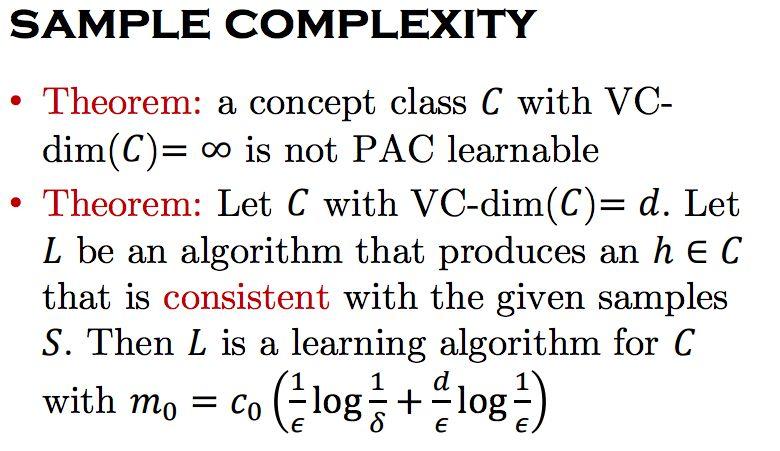
51 PAC LEARNING ALGORITHM PAC Learning algorithm/machine/agent L: A function L : Z H from the training examples to H, such that for every ɛ, δ > 0 there exists a number m 0 (ɛ, δ) such that for every m m 0 and every X, if m examples Z are drawn from P (X, Y ) then: P r[err(h) ɛ] 1 δ, where h H is the hypothesis learned by L according to Z, that is, L(Z) = h The hypothesis space H is (PAC-)learnable if there is a learning algorithm L for H In other words, if a learning algorithm L returns a hypothesis h that is consistent with at least m 0 examples (i.e., it classifies them correctly) then with a probability of at least 1 δ, L has an generalization error of at most ɛ It is PAC! (h lies in H P AC ) The number m 0 (ɛ, δ) of required samples is the sample complexity of the hypothesis space, and is independent of P. It depends on the characteristics of H and on X Unfortunately this bound is typically very large :( 49

52 VALUE OF THE SAMPLE COMPLEXITY All hypotheses in H bad are such that the expected generalization error is greater than ɛ: err(h) > ɛ, h H bad What is the probability that a hypothesis h H bad is consistent with the first m 0 samples? (i.e., it classifies them correctly?) By definition, err(h) > ɛ The probability that h agrees with a given single example x i is at most 1 ɛ: P r P [x i : h(x i ) = y t(x i )] 1 ɛ Since all examples are independent, the bound on h being consistent with a set Z of m 0 examples is: P r P [x i, i = 1,..., m 0 : h(x i ) = y t(x i )] (1 ɛ) m 0 The probability that H bad contains at least one consistent hypothesis is bounded by the sum of the individual probabilities of each hypothesis in H bad, therefore, from the previous relation: P (H bad contains a consistent hypothesis) H bad (1 ɛ) m 0 H (1 ɛ) m 0 H e ɛm 0 where the last inequality derives from a general mathematical bound 50

53 VALUE OF THE SAMPLE COMPLEXITY We aim to make the probability P (H bad contains a consistent hypothesis) being less than a small positive number δ: H e ɛm 0 δ In fact, when this is true, the probability that a hypothesis h is an inconsistent one (i.e., belongs to H bad ) after being consistent on m 0 samples is less than δ. In other words, with a probability 1 δ the machine L returns a hypothesis h that has an expected error rate of at most ɛ The required number m 0 of samples that guarantees PAC learning when h shows consistency on all the m 0 samples, is found by solving wrt to m 0 the inequality H e ɛm 0 δ using the logarithms: m 0 1 ( log 1 ) ɛ δ + log H m 0 is the sample complexity of the hypothesis space H The sample complexity is to the log of cardinality of the hypothesis space, such that it explodes for large numerable spaces and it is not defined for infinite spaces The concept of VC-dimension extends the notions of analysis of expected the generalization errors to hypothesis sets of infinite cardinality and provides tighter bounds. It provides a substitute for the term log H 51

54 VALUE OF THE SAMPLE COMPLEXITY If H is the set of all Boolean functions h : X {0, 1} and X is an n-dimensional feature space, then H = 2 2n (all possible mappings from n inputs to 2 outputs) m 0 = O(2 n ), it grows exponentially with the number of the input features It is necessary to see almost ALL the possible examples! Intuitively: since H contains all generic mappings h, then, for any set Z of m examples, the set of hypothesis consistent with Z contains equal numbers of hypotheses that would classify a new example x m+1 as 0 and as 1 to assess something about generalization we would need to see all the possible examples. To obtain useful results for generalization to new, unseen examples, one way is to restrict H, avoiding to be too general. However, this might remove the possibility to have PAC learning, since H might not include any feasible hypothesis function in the ɛ-ball. 52

55 OUTLINE 1 Supervised learning: classification Non-linear regression/classification, overfitting, and model selection PAC learning and generalization bounds VC-dimension and generalization bounds

56 BETTER BOUNDS USING VC-DIMENSION This is what we will obtain using the VC-dimension... 54

57 DEFINITIONS: SET SHATTERING AND VC-DIMENSION Shattering: Let H be a hypothesis space (also called a concept class) defined over an instance (feature) space X. Let Z = {x 1, x 2,..., x m} X a subset (of examples) from the instance space. The concept class H shatters ( to break into pieces ) Z if every possible function on Z can be represented by some h H. A function on Z is a mapping from an input x to an output y. Restricting the reasoning that follow to binary classification tasks where y {0, 1}, we can rephrase it saying that a set of instances Z is shattered by H if for any binary labeling of the elements in Z there is a consistent hypothesis in H (i.e., there is a choice of the learning parameters θ such that the training error goes to zero). The number of possible mappings (i.e., binary labelings) on Z is equal to 2 Z Vapnik-Chervonenkis (VC) dimension: V C(H) is the maximum number of points that can be shattered by H (i.e., the maximum cardinality of a set shattered by H). The VC-dimension is is the maximum does not exist. 55

58 SHATTERING 3 POINTS IN R 2 WITH CIRCLES All possible binary labelings of a set Z of three points in the plane Can we find circle functions that shatter the set for all possible labelings? Circles must separate the negative (blue) labels from the positive (white) ones: circles must either enclose all negatively labeled points without enclosing any positively labeled point, or vice versa. It does not matter which class is which, since swapping the labels would only require the classifier to be inverted (i.e., to change sign). 56

59 SHATTERING 3 POINTS IN R 2 WITH CIRCLES Every possible labeling can be covered by a circle, so we can shatter the 3 points set 57

60 SHATTERING 3 POINTS IN R 2 WITH CIRCLES We should be precise when defining the class of functions h we are considering In this case, the class is h(x 1, x 2 ) = a [ (x 1 c 1 ) 2 + (x 2 c 2 ) 2] r 2, that is circles centered in (c 1, c 2 ) of radius r. The coefficient a can be +1 or -1. If a = +1, sign(h(x 1, x 2 )) > 0 classifies as 1 the samples falling outside of the circle, and 0 those falling inside the circle. Vice versa when a < 0. Therefore, in the case of the example, the circle is around the white ( 1 ) labeled sample, but the classifier can still correctly classify the blue ( 0 ) samples as negative ones using a = +1. In general, we can assume that we use functions such that the sign of the classifier can be inverted 58

61 OTHER SHATTERING EXAMPLES IN 2D In the first row, h(x 1, x 2 ) = x x2 2 r2, and the classifier is as usual the sign(h(x 1, x 2 )) function. The last case can t be shattered, differently from the previous example, since the parameter a is missing, and the sign function classifies as positive what is outside of the origin-centered circle, while the white point would lie inside the circle. There is no way to place a circle centered in the origin such that the two samples are classified correctly: the circle will always enclose the blue point and classify the white point in the same way. In general, it doesn t matter how the two points are placed, such a situation will always arise since one the two points is necessarily closer to the origin than the other. In the second row, h θ (x 1, x 2 ) = θ 1 x 1 + θ 2 x 2 + θ 0. It s always possible to find a vector θ such that the function h θ (an oriented line) correctly classifies three points, as long as they are not collinear (i.e., as long as they are in general positions) 59

62 SHATTERING FOUR POINTS IN 2D There s no way to shatter four points using circles, since the labeling in the figure won t be feasible for a circle (left) It s however possible using ellipsis (center) There s no way to shatter four points using lines, again the labeling in the figure is not achievable by a linear separator (right) 60

63 MEASURING THE VC-DIMENSION The quantify the VC-dimension of a concept class H over an instance space X: 1 Demonstrate it can shatter one set of size n (lower bound). This does not mean that H can shatter any set of size n! 2 Demonstrate it cannot shatter any set of size n + 1 (upper bound). For all n + 1-dimensional sets there is (at least) one labeling that can t be shattered Over a R 2 instance space, a linear classifier (oriented line) h θ (x 1, x 2 ) = θ 1 x 1 + θ 2 x 2 + θ 0 can shatter sets of 3 points (as long as they are not collinear) but cannot shatter any set of four points. Therefore, the VC-dimension of a linear learning machine over R 2 is 3. The result can be generalized: the VC-dimension of the set of the oriented hyperplanes in R n is n + 1. The VC-dimension of axis-aligned hyperplanes is also n + 1. In fact, as a special case of the general oriented hyperplanes, it s possible to find an n-dimensional example, but it would clearly fail shattering in the n + 1-dimensional case Over a R 2 instance space, the VC-dimension of general circle functions is 3. Instead, for origin-centered circles, the VC-dimension is 2 (they can clearly consistently classify set of one element, but not sets of two elements) The VC-dimension gives concreteness to the notion of power (capacity) of a learning machine: an upper bound on the number of examples that a class of hypothesis could consistently classify 61

64 AXIS PARALLEL RECTANGLES IN 2D X is the set of all points in R 2 H is the set of all axis parallel rectangles in 2D (Left) V C 3 since there is a placement of 3 points that can be shattered (Right) V C 4 since there is a placement of 4 points that can be shattered (Middle) V C = 4 since for all placements of 5 points, there exists a labeling that can t be shattered Figures from Barnabás Póczos 62

65 INTERVALS ON THE REAL LINE The concept class is defined by two parameters θ 1 and θ 2 in [0,1], that define an interval [θ 1, θ 2 ] on the real line. A concept function tags an input sample x (0, 1) as positive if θ 1 x θ 2, and negative otherwise. VC-dim 2. Selected a sample of 2 points x 1 and x 2 in (0, 1), we need to show that there are values of θ 1 and θ 2 which realize all the possible four labelings: {(+, +), (, ), (+, ), (, +)}. This is clearly possible as one can place the interval [θ 1, θ 2 ] such that the intersection with the interval [x 1, x 2 ] is null, (thus producing (-, -)), or to fully include [x 1, x 2 ] (thus producing (+, +)) or to partially intersect [x 1, x 2 ] such that x 1 or x 2 are excluded (thus producing the remaining two labelings). VC-dim cannot be more that 2, since any sample of three points {x 1, x 2, x 3 } on the line (0, 1) cannot be shattered (x 1 < x 2 < x 3 ). It is sufficient to show that one of the labelings is not realizable: in particular, the labeling (+, -, +) cannot be realizable by any interval [θ 1, θ 2 ] because if x 1, x 3 are labeled positive then by definition the interval [θ 1, θ 2 ] must fully include the interval [x 1, x 3 ] and since x 1 < x 2 < x 3 then x 2 must be labeled positive as well, which makes the labeling unfeasible. 63

66 ADDITIONAL SOURCES More examples, as well as an accessible treatment of the topics related to the VC dimension and PAC learning can be found in The following are the slides from Emma, that summarize the results deriving from the use of the VC dimension 64

67

68

69

70

71

72

73