MULTI VARIABLE OPTIMIZATION

Size: px

Start display at page:

Download "MULTI VARIABLE OPTIMIZATION"

Daniel Freeman
5 years ago
Views:

1 MULI VARIABLE OPIMIZAION Min f(x 1, x 2, x 3,----- x n ) UNIDIRECIONAL SEARCH - CONSIDER A DIRECION S r r x( α ) = x +α s - REDUCE O Min f (α) - SOLVE AS A SINGLE VARIABLE PROBLEM Min Point s r

2 Uni directional search (example) Min f(x 1, x 2 ) = (x 1-10) 2 + (x 2-10) 2 S = (2, 5) (search direction) X = (2, 1) (Initial guess)

3 DIREC SERACH MEHODS - SEARCH HROUGH MANY DIRECIONS - FOR N VARIABLES 2 N DIRECIONS -Obtained by altering each of the n values and taking all combinations

4 EVOLUIONARY OPIMIZAION MEHOD - COMPARE ALL 2 N +1 POINS & CHOOSE HE BES. - CONINUE ILL HERE IS AN IMPROVE MEN - ELSE DECREASE INCREAMEN SEP 1: x 0 = INIIAL POIN i = SEP REDUCION PARAMEER FOR EACH VARIABLE = ERMINAION PARA MEER

5 2 & 2 ; 2 / 4 : 1) (2 3: 2 / 2 2 : 0 0 GOO x x ELSE GOO x x IF SEP Min x SEP x x POINS CREAE ELSE SOP IF SEP i i N i i i N = = = + = ± = <

7 Hooke Jeeves pattern search Pattern Search --- Create a set of search directions iteratively Should be linearly independent A combination of exploratory and pattern moves Exploratory find the best point in the vicinity of the current point Pattern Jump in the direction of change, if better then continue, else reduce size of exploratory move and continue

8 Exploratory move Current solution is x c ; set i = 1; x = x c S1: f = f(x), f + = f(x i + i ), f - = f(x i - i ) S2: f min = min (f, f +, f - ); set x corresponding to f min S3: If i = N, go to 4; else i = i + 1, go to 1 S4: If x x c, success, else failure

9 Pattern Move S1: Choose x (0), I, for I = 1, 2, N, ε, and set k = 0 S2: Perform exploratory move with x k as base point; If success, x k+1 = x, go to 4 else goto 3 S3: If < ε, terminate Else set i = i / α --- i, go to 2

10 Pattern Move (contd) S4: k = k+1; x k+1 p = x k + (x k x k-1 ) S5: Perform another exploratory move with x k+1 p as the base point; Result = x k+1 S6: If f(x k+1 ) < f(x k ), goto S4 Else gotos3

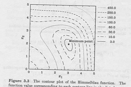
11 Example : Consider the Himmelblau function: f ( x, x2) = ( x1 + x2 11) + ( x1 + x2 7 Solution Step 1 Selection of initial conditions 1. Initial Point : (0) x = (0,0) 2. Increment vector : 3. Reduction factor : α = 2 4. ermination parameter : ε = Iteration counter : k = ) = (0.5,0.5)

13 Step 2 Perform an Iteration of the exploratory move with base point as x = x (0) hus we set x (0) = x = (0,0) and i = 1 he exploratory move will be performed with the following steps

14 Steps for the Exploratory move Step 1 : Explore the vicinity of the variable x1 ( Calculate the function values at three points (0) (0) x + 1x ) = (0.5,0.5) f = f (( 0.5,0.5) ) = (0) x = (0,0) f = f (( 0,0) ) = 170 ( (0) (0) x 1x ) = ( 0.5,0.5) = f (( 0.5,0.5) ) = Step 2 : ake the Minimum of above function and corresponding point Step 3 : As i 1 : all variables are not explored Increment counter i=2 and explore second variable. First iteration completed f

15 Step1: At this point the base point is x = (0.5,0) explore the variable x2 and calculate the function values. f = f (( 0.5,0.5) ) = f = f (( 0.5,0) ) = f = f (( 0.5, 0.5) ) = Step 2 : fmin = and point, x=(0.5,0.5) Step 3 : As i=2 move to the step 4 of the exploratory move Step 4 : ( of the Exploratory move ) c Since x x the move is success and we set x = (0.5,0.5)

16 (1) As the move is success, set x = x = (0.5,0.5) move to step 4 x SEP 4 : We set k=1 and perform Pattern move (2) p = ( x (1) + ( x (1) x (0) ) ) = 2(0.5,0.5) Step 5 : Perform another exploratory move as before ( 2) and with x p as the base point. he new point is x = (1.5,1.5) (2) Set the new point x = x = (1.5,1.5 ) (2) (1) Step 6 : f ( x ) = is smaller than f ( x ) = Proceed to next step to perform another pattern move (0,0) = (1,1)

17 SEP 4 : Set k=2 and create a new point (2) (1) Note: as x is better than x, a jump along the direction (2) ( x x true minimum (3) (2) (1) x p = (2x x ) = (2.5,2.5) (1) ) is made, this will take search closer to SEP 5 : Perform another exploratory move to find any better point around the new point. Performing the move on both variables we have New point (3) x = (3.0,2.0) his point is the true minimum point

18 In the example the minimum of the Hookes-Jeeves algorithm happen in two iterations : this may not be the case always Even though the minimum point is reached there is no way of finding whether the optimum is reached or not he algorithm proceeds until the norm if the increment vector is small. SEP 6 : function value at new point 3 2 f ( x ) = 0 < f ( x ) = hus move on to step 4

19 SEP 4 : he iteration counter k = 3 and the new point (4) (3) (2) x p = (2x x ) = (4.5,2.5) SEP 5 : With the new point as base the search is success and x=(4.0,2.0) and thus we set (4) x = (4.0,2.0) SEP 6 : he function value is 50, which is larger that the earlier i.e. 0. hus we move to step 3 Step 3 : Since = 0. 5 ε we reduce the increment vector = ( 0.5,0.5) / 2 = (0.25,0.25) and proceed to Step 2 to perform the iterations

20 Step 2 : Perform an exploratory move with the (3) following as current point x = (3.0,2.0) he exploratory move on both the variables is failure (3) and we obtain x = (3.0,2.0) thus we proceed to Step 3 Step 3 : Since is not small reduce the increment vector and move to Step 2. he new increment vector is = (0.125,0.125) he algorithm now continues with step 2 and step 3 until is smaller than the termination factor. he final solution is x * = (3.0,2.0 ) with the function value 0

21 POWELL S CONJUGAE DIRECION MEHOD For a quadratic function IN 2 VARIABLES - AKE 2 POINS x 1 & x 2 AND - A DIRECION d IF y 1 IS A SOLUION OF MIN f ( x 1 + λd) & y 2 IS A SOLUION OF MIN f ( x 2 + λd) HEN (y 2 -y 1 ) IS CONJUGAE O d OPIMUM LIES ALONG (y 2 -y 1 ) y 2 x 2 y 1 x 1

22 OR FROM x 1 GE y 1 ALONG (1,0) y 1 GE x 2 ALONG (0,1) x 2 GE y 2 ALONG (1,0) AKE (y 2 -y 1 )

23 Alternate to the above method - One point ( x 1 ) and both coordinate directions ((1,0) and (0,1) ) - Can be used to create a pair of conjugate 2 1 directions ( d and ( y y ))

24 Point ( y 1 ) obtained by unidirectional search along ( 1,0) from the point ( x 1 ). Point ( x 2 ) obtained by unidirectional search along from the point ( y 1. ( 0,1) ) Point ( y 2 ) obtained by unidirectional search along (1,0) from the point ( x 2 ). he figure shown also follows the Parallel Subspace Property. his requires hree Unidirectional searches.

25 Example : Consider the Himmelblau function: f ( x , x2) = ( x1 + x2 11) + ( x1 + x2 7) Solution (0) Step1 : Begin with a point x = (0,4) (1) (2) Initial direction s = (1,0) and s = (0,1) Step 2: Find minimum along the first search direction. Any point along that direction can be written as ( ) x p = x (0) + αs (1)

26 hus the point x p can be written as x p =(α,4) Now the two variable function can be expressed in terms of one variable F( α) = ( α 7) + ( α + 9) We are looking for the point which the function value is minimum. == Following the procedure of numerical differentiation. Using the bounding phase method, the minimum is bracketed in the interval (1,4), and using the golden search method the minimum α*=2.083 with three decimals places of accuracy. hus x 1 = (2.083,4.00)

28 Similarly find the minimum point along the second search direction. A general point on the line is 1 2 x ( α) = ( x + αs ) = (2.083, ( α + 4)) Using similar approach as said earlier we have α*= x 2 = (2.083,2.408) From the above point perform a unidirectional search along the first search direction and obtain the minimum point x 3 = (2.881,2.408)

29 Step 3 : According to the parallel subspace property, we find the new conjugate direction (2) s = (1,0) Step 4 : the magnitude of search vector d is not small. hus the new conjugate search direction are s (1) = (0.798, 1.592) / (0.798, 1.592) = (0.448, 0.894) his completes one iteration of Powell s conjugate direction method.

30 Step 2 : A single variable minimization along the search direction s (1) from the point x (3) =(2.881,2.408) results in the new point x = (3.063,2.045) One more unidirectional search along the s 2 from the point x 4 results in the point x 5. Another minimization along s 1 results in x 6 Step 3 : the new conjugate direction is (6) (4) d = ( x x ) = (0.055, 0.039) he unit vector along this direction is ( 0.816,-0.578)

31 Step 4 : he new pair of conjugate search direction are (1) (2) s = (0.448, 0.894) s = (0.055, 0.039) he search direction d ( before normalizing ) may be considered to be small and therefore the algorithm may be terminated

32 EXENDED PARALLEL SUBSPACE PROPERY. Let us assume that the point y 1 is found after unidirectional searches along each of m ( < N ) conjugate directions from a chosen point x 1 and 2 similarly, the point y is found after unidirectional searches along each of m conjugate directions from another point x 2. he 2 1 vector ( y y ) is the conjugate to all m search directions.

33 ALGORIHM Step 1 : Choose starting point And a set of N linearly independent direction Step 2 : Minimize along N unidirectional search directions using the previous minimum point to begin the next search. Step 3 : Form a new conjugate direction d using the extended parallel subspace property. Step 4 : If d is small or search directions are linearly dependent, ERMINAE, Else replace starting point for N directions, set s (1) =d / d And go to Step 2

34 FOR N VARIABLES SEP 1: AKE x 0 & N LINEARLY INDEPENDEN DIRECIONS s 1, s 2, s 3, s 4, s N s i = e i SEP 2: - MINIMIZE ALONG N UNI-DIRECIONAL SEARCH DIRECIONS,USING PREVIOUS BES EVERY IME - PERFORM ANOHER SEARCH ALONG s 1 SEP 3: FROM HE CONJUGAE DIRECION d SEP 4: IF d IS SMALL ERMINAE ELSE s j j 1 = s j & s 1 = d / d GOO 2

35 Powell s method with N variables Start from x 1 Get y 1 by doing search along s 1 Find y 2 by doing search along s 2, s 3, s 4.. s n, s 1 (y 2 y 1 ) is conjugate to s 1 Replace s n by (y 2 -y 1 ) and start same procedure starting from s 2

36 GRADIEN BASED MEHODS he methods exploit the derivative information of the function and are faster. Cannot be applied to problems where the objective function is discrete or discontinuous. Efficient when the derivative information is easily available Some algorithms require first order derivatives while some require first and second order derivatives of the objective function. he derivatives can be obtained by numerical computations

37 Methods in Gradient Search. Decent Direction Cauchy s (steepest decent) method Newton s Method Marquardt s Method Conjugate gradient method Variable-metric method

38 (t) By definition, the first derivative f ( x ) at any (t) point ( x ) represents the direction of the maximum increase of the function value. If we are interested in finding a point with the minimum function value, ideally we should be searching along the opposite to the first derivative direction, that is, we should search (t) along f ( x ) Any search made in this direction will have smaller function value.

39 DECEN DIRECION (t) A search direction ( d ) is a decent direction at a (t) ( t) ( t) point ( x ) if the condition f ( x ). d 0 is (t) satisfied in the vicinity of the point ( x ) It can also be proved by comparing function values at two points along any decent direction. ( t) ( t) he magnitude of the vector f ( x ). d for a (t) decent direction ( d ) specifies how decent the search direction is. he above statement can be explained with the help of an example on the next side

40 If ( t) ( t). d ( ) is used, the quantity 2 = f x is maximally negative f ( x ( t) ). d ( t) (t) hus the search direction f ( x ) is called the steepest decent direction Note : = x x x1 2 3 x n

Example Consider the Himmelblau function: f ( x 2 2 2 2 1, x2) = ( x1 + x2 11) + ( x1 + x2 7) We would like to determine

41 Example Consider the Himmelblau function: f ( x , x2) = ( x1 + x2 11) + ( x1 + x2 7) We would like to determine whether the direction ( t) ( t ) ( d ) = (1,0 ) at the point ( x ) = (1,1 ) is a decent direction or not. Refer to the figure below

42 It is clear from the figure that if we move locally (t) (t) along ( d ) from the point ( x ) will reduce the function value Investigate this aspect by calculating the (t) derivative f ( x ) at the point. Derivative as calculated numerically is ( t) f ( x ) = ( 46, 38) (t) aking the dot product we obtain f ( x ) and ( x f ( x ( t) ) d( t) = ( 46, 38) = 46 he above is a negative quantity, thus the search direction is a Decent direction 1 0 (t) )

43 he amount of non-negativity suggests the extent of decent in the direction ( t) If the search direction d ( t) = f ( x ) = ( 46, 38) is used, the magnitude of the above dot product is 46 ( 46, 38) = 3, he direction (46,38) or (0.771,0.637) is more descent than he above direction is the steepest direction at the point x (t)

44 In nonlinear function the steepest decent direction at any point may not exactly pass through the true minimum. he steepest decent direction is a direction which is a local best direction It is not guaranteed that moving along the steepest decent direction will always take the search closer to the true minimum

45 CAUCHY S ( SEEPES DECEN) MEHOD Search direction used is the negative of the gradient at any particular point x (t) : k s = f ( x (k ) ) As the direction gives the maximum decent in function values, it is also known as Steepest Decent Methods he algorithm guarantees improvement in the function value at every iteration

46 Algorithm in brief ; At every iteration ; o find the minimum point along direction Compute derivative at current point Perform unidirectional search in the negative to this derivative direction he minimum point becomes the current point and the search continues from this point ; Algorithm continues until a point having a small enough gradient vector is found.

47 Algorithm in Steps SEP 1: CHOOSE M (MAX. NO. OF IERAIONS) SEP 2: CALCULAE 1, 2, x 0, k = 0 f ( x k ) SEP 3: IF f ( x k ) 1 ERMINAE IF k M ERMINAE SEP 4: UNIDIRECIONAL SEARCH USING 2

48 MIN. f( x k+ 1 ) = f( x k α f( x k )) SEP 5: IF x k+ 1 x x k k k= k+ 1 ELSE GOO SEP MEHOD WORKS WELL WHEN x k IS FAR FROM x * (OPIMUM) - IF POIN IS CLOSE O x * HEN CHANGE IN GRADIEN VECOR IS VERY SMALL. - OHER MEHODS USE VARIAION -SECOND DERIVAIVES(NEWON S) -COMBIMAION -CONJUGAE GRADIEN MEHOD

49 Example Consider the Himmelblau function: f ( x , x2) = ( x1 + x2 11) + ( x1 + x2 7) Step 1: Choose large value of M for proper convergence M 100 is normally chosen. Initial conditions : M = 100 x (0) = (0,0) ε 1 = ε 2 =10-3 k=0

50 Step 2 : he derivative at the initial point x 0 calculated and is found to be (- 14, - 22) is Step 3 : As the magnitude of the derivative is not small and k = 0 < M = 100. do not terminate proceed to step 4

51 Step 4 : perform a line search form x (0) in the direction (0) f ( x ) such that the function value is minimum. Along that direction, any point can be expressed by fixing a value for the parameter α 0 in the equation. x = x 0 ( α,22 ) 0 (0) α f ( x ) = α Using Golden section search in the interval (0,1) α 0* = minimum point along the direction is x 1 = (1.788,2.810) Step 5 : As x 1 and x 0 are quite different, we do not terminate, but go back to step 2, this completes one iteration.

52 Step 2: he derivative vector at this point is ( , ) Step 3 : he magnitude of the derivative vector is not smaller than ε1, thus, we continue with step 4. Step 4 : Another unidirectional search along ( , ) from the point x1=(1.788,2.810) using the golden section search finds the new point x2=(23.008,1.99) with a function value equal to Continue the process until the termination criteria is reached

53 Penalty function approach ransformation method - convert to a sequence of unconstrained problems. Give penalty to (violated) constraints. Add to objective function. Solve. Use result as starting point for next iteration. Alter penalties ands repeat.

54 Minimise Subjected to Penalty = ( x x2 11) + ( x1 + x2 7) 2 2 ( x1 5) + x ( x1 5) < x > Feasible region Minimum point Infeasible region x 2 x 1

55 1. Choose Process 2. Form modified objective function P( x k 3. Start with x. Find k + 1 so as to minimize P. 4. If k, R P k ) = f ε,, 1 ε 2 R, Ω. ( x k ) + Ω( R k, g( x (use ) ε 1 k 1 1 ( + k k x, R ) P( x, R k ) < ε 2 ), h( x erminate Else R k + = cr, k=k+1; go to step 2. x k k ))

56 At any stage minimize P(x,R) = f(x)+ω(r,g(x),h(x)) R = set of penalty parameters Ω= penalty function

59 ypes of penalty function Parabolic penalty 2 Ω = R{h(x)} - for equality constraints - only for infeasible points Interior penalty functions - penalize feasible points Exterior penalty functions - penalize infeasible points Mixed penalty functions - combination of both

60 Infinite barrier penalty Ω = R g (x) j - inequality constraints. - R is very large. -Exterior. Log penalty Ω=-R ln[g(x)] -inequality constraints - for feasible points -interior. -initially large R. - larger penalty close to border.

61 Inverse penalty 1 Ω = R g( x) -interior. - larger penalty close to border. - initially large R Bracket order penalty R < g( x) > 2 - <A>=A if A<0. -exterior. - initially small R.

62 Direct search Variable elimination - for equality constraints - Express one variable as a function of others and - Eliminate one variable - Remove all equality constraints

63 Complex search - generate a set of points at random - If a point is infeasible reflect beyond centroid of remaining points - ake worst point and push towards centroid of feasible points.

64 Complex Search Algo S1: Assume a bound in x (x L, x U ), a reflection parameter α, and ε & δ S2: Generate a set of P (= 2N) initial points For each point Sample N times to determine x (P) i, in the given bound if x (P) is infeasible, calculate x (centroid) of the current set of points and set x P = x P +1/2(x-x P ) until x P is feasible. If x P is feasible, continue till u get P points

65 Complex Search Algo (contd) S3: Reflection step select x R such that f(x R ) = max (f(x P )) = F max calculate x, centroid of remaining points x m = x + α (x -x R ) If x m is feasible and f(x m ) > F max, retrtact half the distance to x, and continue till f(x m ) < F max If x m is feasible and f(xm) < Fmax, Go to S5 If x m is infeasible, Goto S4

66 Complex Search Algo (contd) S4: Check for feasibility of the solution For all i, reset violated variable bounds if x im < x il, x im = x i L if x im > x iu, x im = x i U If the resulting x im is infeasible, retract half the distance to the centroid, repeat till x m is feasible

67 Complex Search Algo (contd) S5: Replace x R by x m, check for termination f mean = mean of f(x P ), x mean = mean (x P ) p ( f ( x p ) f mean 2 ) ε p x p x mean 2 δ

68 Complex Search Algo (contd)

69 Characteristics of complex search For complex feasible region If the optimum is well inside the search space, the algo is efficient Not so good if the search space is narrow, or the optimum is close to the constraint boundary

Optimization Concepts and Applications in Engineering

Optimization Concepts and Applications in Engineering Ashok D. Belegundu, Ph.D. Department of Mechanical Engineering The Pennsylvania State University University Park, Pennsylvania Tirupathi R. Chandrupatia,