EAD 115. Numerical Solution of Engineering and Scientific Problems. David M. Rocke Department of Applied Science

Transcription

1 EAD 115 Numerical Solution of Engineering and Scientific Problems David M. Rocke Department of Applied Science

2 Taylor s Theorem Can often approximate a function by a polynomial The error in the approximation is related to the first omitted term There are several forms for the error

3 ( n) f ''( a) 2 f ( a) n f ( x) = f( a) + f '( a)( x- a) + ( x- a) + + ( x- a) + R 2! n! x n ( x-t) ( n+ 1) Rn = f () t dt R= ò a n! ( x-a) ( n + 1)! n+ 1 f ( n+ 1) ( x) n ( n) f ''( x) 2 f ( x) n f ( x+ h) = f( x) + f '( x) h+ h + + h + R 2! n! n+ 1 h ( n+ 1) R= f ( x) ( n + 1)! n

4 Series Truncation Error In general, the more terms in a Taylor series, the smaller the error In general, the smaller the step size h, the smaller the error Error is O(h n+1 ), so halving the step size should result in a reduction of error that is on the order of 2 n+1 In general the smoother the function the smaller the error

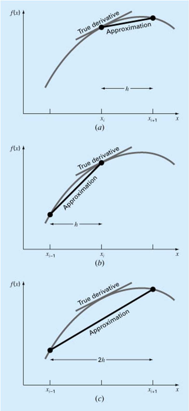
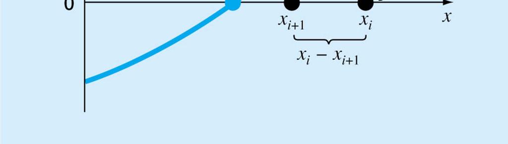
5 Numerical Differentiation f ( xi+ 1) = f( xi) + f '( xi)( xi+ 1- xi) + Oé êë ( xi+ 1-xi) f '( xi)( xi+ 1- xi) = f( xi+ 1) - f( xi) + Oé êë ( xi+ 1-xi) f( x )- f( x ) f x Oé x x ù û i+ 1 i '( i) = + ( i+ 1 - i) ( xi+ 1 - xi) ë Dfi f '( xi ) = + O( h) h 2 2 ù úû ù úû First Forward Difference

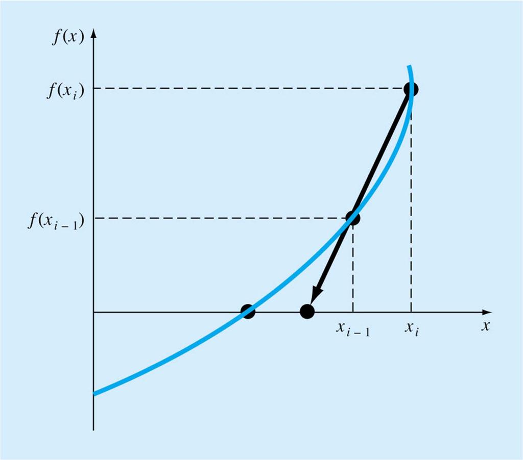
6 f ( x ) = f( x )- f '( x ) h+ O( h ) i-1 i i f( x )- f( x ) f '( x ) = i i-1 + O( h) i h f f '( x ) = i + O( h) i h 2 First Backward Difference

7 i+ 1 i i i i-1 i i i i+ 1 i-1 i i+ 1 i-1 i f ( x ) = f ( x ) + f '( x ) h+ 0.5 f ''( x ) h + O( h ) 2 3 f ( x ) = f ( x )- f '( x ) h+ 0.5 f ''( x ) h + O( h ) f( x )- f( x ) = 2 f '( x ) h+ O( h ) f( x ) = f( x ) + 2 f '( x ) h+ O( h ) f( x )- f( x ) f '( x ) = i+ 1 i-1 + O( h 2 ) i 2h First Centered Difference

8

9 Second Forward Difference f x f x h h f x f x ''( i) D ( i) / = D ( i+ 1) - ( i) ( ) f x h é êë f x f x f x f x -2 f ''( xi) h éf( xi+ 2) - 2 f( xi+ 1) + f( xi) ù ë û -2 ''( i) ( i+ 2) - ( i+ 1) - ( i+ 1) - ( i) ( ) ( ) ù úû

10 Propagation of Error Suppose that we have an approximation of the quantity x, and we then transform the value of x by a function f(x). How is the error in f(x) related to the error in x? How can we determine this if f is a function of several inputs?

11 x x x = x+ e f ''( x) f( x ) = f( x) + f '( x) e+ e 2 + 2! f( x )- f( x) = f '( x) e If the error is bounded e < B f( x )- f( x) < f '( x) B If the error is random with standard deviation SD( x ) = s s SD( f ( x )) f '( x) s

12 x x x = x + e x x x = x + e f( x, x ) = f( x, x ) + f ( x, x ) e + f ( x, x ) e f( x, x )- f( x, x ) f ( x, x ) e + f ( x, x ) e If the errors are bounded e i < B i f( x, x ) f( x, x ) f ( x, x ) B f ( x, x < ) B2

13 Stability and Condition If small changes in the input produce large changes in the answer, the problem is said to be ill conditioned or unstable Numerical methods should be able to cope with ill conditioned problems Naïve methods may not meet this requirement

14 x = x+ e The error of the input is e. e/ x e/ x is the relative error of the input. The error of the output is f( x )- f( x) e f '( x) and the relative error of the output is ef '( x) ef '( x ) f( x) f( x ) The ratio of the output RE to the input RE is e f '( x) xf '( x) xf '( x ) = ( e / x) f( x) f( x) f( x )

15 Bracketing Methods Find two points x L and x U so that f(x L ) and f(x U ) have opposite signs If f() is continuous, there must be at least one root in the interval Bracketing methods take this information, and produce successive approximations to the solution by narrowing the interval bracketing a/the root

16 Behavior of Roots of Continuous Functions If the function values at two points have the same sign, then the number of roots between them is even, including possibly 0. If the function values at two points have different signs, then the number of roots between them is odd, so cannot be 0.

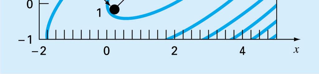
17 Exceptions Roots of multiplicity greater than one, count as multiple roots in this. The function f( x) ( x 1) 2 has only one root at x = 1, even though the function does not change sign in the interval from 0 to 2. Discontinuous functions need not obey the rules.

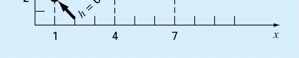
18 Bisection Method Suppose a continuous function changes sign between x L and x U. Consider x M =(x L + x U )/2 If f(x M ) = 0, we have found a root. If f(x M ) is not zero, it differs in sign from exactly one of the end points This gives a new interval of half the length which must contain a root

19 Error Estimate for Bisection Interval at start of step i is 2 x, the distance between the upper and lower bounds. We pick the middle of this interval as the i th guess The next interval has length x, has one end on the previous guess, and the other at one end or the other of the previous interval

20 At step i the error cannot be greater than x and at step i+1 it cannot be greater than x/2 The distance between the best guess at step i and the best guess at the next step is exactly x/2 Thus, the error bound is the change in the best guess

21 Function Evaluations In some applications, evaluation of the function to be minimized is expensive and may itself involve a large computation In n iterations, the naive implementation uses 2n function evaluations. The implementation that saves and reuses function values uses n + 1 function evaluations

22 In n iterations, the first implementation uses 2n function evaluations. The second implementation use n + 1 function evaluations Neither implementation contains a check that the function actually does change sign in the input interval

23 Summary of Bisection The method is slow but sure for continuous functions There is a well-defined error bound, though the true error may be much less

24 Method of False Position Also called linear interpolation or regula falsi. Bisection uses information that there is a root in the interval x L to x U but does not use any information from the function values f(x L ) and f(x U ). False position uses the insight that if f(x L ) is smaller than f(x U ), one would expect the root to lie closer to x L.

25 Fig 5.12

26 The line through the two end points of the interval is f( x )- f( x ) y- f( xu) = x-x x - x ( ) L U ( ) This intersects the x axis where x satisfies f( xl) - f( xu) - f( xu) = x-x x - x ( ) x L ( ) xl- xu x- xu =- f( xu) f( x )- f( x ) R = x - U L L U U f( xu)( xl- xu) f ( x )- f( x ) L U U U U

27 The new root estimate x R replaces whichever of the end points that has the same sign as f(x R ), so that the two new endpoint still bracket the root. We use as an error estimate, the change in the best root estimate from one iteration to the next. This works well to the extent that the function is nearly linear in the interval and near the root.

28 Pitfalls of False Position If the function is very nonlinear in the bracketing interval, convergence can be very slow, and the approximate error estimate can be very poor. A possible solution is to use bisection until the function appears nearly linear, then switch to false position for faster convergence, or to use false position, but switch to bisection if convergence is slow. Another is to adjust a fixed endpoint

29 Fig 5.14

30 Results of Modified False Position With the function x 10 1 and starting points 0 and 1.3, bisection takes 14 iterations to achieve a relative error of = 0.01%. False Position takes 39 iterations. The modifications of false position take 12 iterations each.

31 Modified False Position

32 Modified False Position

33 Open Methods of Root Finding Bracketing methods begin with an interval that is known to contain at least one root. These methods are guaranteed to find a root eventually, though they may be slow. Open methods begin only with a point guess. They are not guaranteed to converge, but may be much faster.

34 When does a fixed-point iteration converge? Solve gx ( )- x= 0 x x i+ 1 r = = g( x ) i g( x ) r x - x = g( x )-g( x ) r i+ 1 r i

35 x- x = gx ( )-gx ( ) r i+ 1 r i gx ( r) - gx ( i) g '( x) = (Derivative Mean Value Thm) x - x ( x - x ) g'( x) = g( x )-g( x ) x - x = ( x -x ) g'( x) E r i+ 1 r i ti, + 1 ti, r r i r i = E g'( x) i Thus the error at iteration i+1 is smaller than the error at iteration i so long as the derivative is less than 1 in absolute value in a neighborhood of the root. Linearly convergent with constant c bounded by the maximum derivative of g().

36 Newton-Raphson Beginning with a point, its function value and its derivative, derive a new guess Project the tangent line until it intersects the x-axis Approximate the function by a first order Taylor series, and solve the approximate problem exactly

37 Fig 6.5

38 f( x) f( x ) + f '( x )( x- x ) = 0 i i i f '( x )( x- x ) =-f( x ) i i i x- x =-f( x )/ f '( x ) i i i x= x - f( x )/ f '( x ) i i i

39 Error Analysis Newton-Raphson appears to converge quadratically, so that E i+1 = c E 2 i This convergence is extremely rapid, and occurs under modest conditions once the iterate is close to the solution.

40 The exact Taylor series expansion of f( x) f( x ) = 0 = f( x ) + f '( x )( x - x ) f ''( x)( x -x ) The Newton-Raphson iteration is based on the truncated series f( x) = f( x ) + f '( x )( x-x ) leading to the iteration x i+ 1 r i i r i r i = x - i i i f( x )/ f '( x ) i i i or 0 = f( x ) + f '( x )( x -x ) i i i+ 1 i 0 = f '( x )( x - x ) f ''( x)( x -x ) i r i+ 1 r i 2 2

41 0 = f '( x )( x - x ) f ''( x)( x -x ) i r i+ 1 r i 0 = f '( x ) E f ''( x) E E =- 2 i t, i+ 1 t, i f ''( x) E 2 ti, + 1 ti, 2 f '( xi ) 2

42 Pitfalls of Newton-Raphson When close to a solution, and when the conditions are satisfied (e.g., f (x r ) is not 0), Newton-Raphson converges rapidly. When started farther away, it may diverge or converge slowly at first. The quadratic convergence applies only once the solution is close.

43 Safeguards for Newton-Raphson On each iteration, one can keep track of f(x). If the new proposed iterate has a larger value of this quantity, then replace it by a step half as big. The same trick can be used for keeping the iterations away from undesirable regions (non-positive numbers for the log function). One can simply return a very large number instead of NaN.

44 The Secant Method For some functions, it is difficult to calculate the derivative We can use a backward difference to approximate the derivative, and then use a Newton-Raphson type calculation This is called the secant method

45 Fig 6.7

46 f( xi- 1) - f( xi) f '( xi ) xi- 1 - xi f ( x ) f ( x )( x - x ) x = x - x - '( ) ( ) ( ) i i i-1 i i+ 1 i i f xi f xi- 1 - f xi The secant method is similar to Newton- Raphson It appears similar to false position, but this is not the case.

47 Multiple Roots Multiple roots are places where the function and one or more derivatives are zero. This is most easily explained for polynomials. Non-polynomials can exhibit the same phenomenon

48 f( x) = ( x-1)( x-2) 2 '( ) ( 2) 2( 1)( 2) 2 has a simple root at x= 1 and a double root at x= 2 f x = x- + x- x- f '(2) = 0 f '(1) ¹ 0 f( x) = ( x-1)( x-2) has a triple root at x = 2 3

49 Multiple roots cause potential trouble for all methods of root finding Bracketing methods may not work if there is an even multiple root in which the function does not cross the axis. An interval in which a continuous function changes sign has at least one root. An interval in which a continuous function does not change sign may or may not have a root Newton-Raphson and secant methods divide by f () which is difficult if it is 0.

50 Solution of multiple linear equations One linear equation Algebra One nonlinear equation Bracketing or open methods Multiple linear equations This chapter Multiple nonlinear equations Open methods mostly

51 Fig PT3.4

52 Matrix representation of linear equations a x + a x + + a x = b n n 1 a x + a x + + a x = b n n 2 a x + a x + + a x = b n1 1 n2 2 nn n n éa a a ùéx ù éb ù n 1 1 úê a21 a22 a úê 2n x 2 b ê úê ú ê 2ú úê = úê êa a a úêx ú êb ú ë n1 n2 nnûë nû ë nû

53 Singularity and the determinant A square matrix is singular if one row can be made up from the other rows by adding and multiplying by constants Equivalent for columns The determinant is 0 for singular matrices, and is a quantitative measure of singularity if not 0

54 Ax = b has a unique solution exactly when A ¹ 0 ( A is nonsingular) If A is singular, either the equation has no solutions or it has many. x+ 2y= 4 x- y= 1 x= 2 y= 1 2x- 2y= 4 x- y= 2 any values such that y= x-2 2x- 2y= 4 x- y= 3 No solution!

55 Gaussian Elimination Manipulate original matrix and vector to eliminate variables Back-substitute to solve equations In most straightforward form, can be subject to problems if certain matrix entries are 0 or small This in turn can be fixed by pivoting

56 a x + a x + + a x = b n n 1 a x + a x + + a x = b n n 2 a x + a x + + a x = b n1 1 n2 2 nn n n éa a a b a a a b êë a a a b n n 2 n1 n2 nn n ù úû

57 a x + a x + + a x = b n n 1 a x + a x + + a x n n -[ a x + ( a a / a ) x + + ( a a / a ) x ] = b -ba / a n n ( a - a a / a ) x + + ( a -a a / a ) x n 1n n = b -ba / a éa11 a12 a 1n 0 a -a a / a a -a a / a êë an 1 an2 ann n 1n b 1 b -ba / a b n ù úû

58 a x + a x + a x + a x = b a x + a x + a x + a x = b a x + a x + a x + a x = b a x + a x + a x + a x = b

59 a x + a x + a x + a x = b ( a - a a / a ) x + ( a - a a / a ) x + ( a - a a / a ) x = b -ba / a ) ( a - a a / a ) x + ( a - a a / a ) x + ( a - a a / a ) x = b -ba / a ) ( a42 - a12a21 / a11) x2 + ( a43 -a13a21 / a11 ) x3+ ( a44- a14a21/ a11) x4 = b4-ba 1 21/ a11) a x + a x + a x + a x = b a x + a x + a x = b a x + a x + a x = b a x + a x + a x = b a x + a x + a x + a x = b a x + a x + a x = b a 33x3 + a 34x4 = b 3 a x = b

60 a x + a x + a x + a x = b a x + a x + a x = b a x + a x = b a x = b x = b / a a x = b -a x a x = b -a b / a x = b / a -a b / a a a x = b - a x + a x a 22x2 = b 2 -a 23( b 3 / a 33 - a 34b 4 / a 33a 44) + a 24( b 4 / a 44) x = b / a -a b / a a - a a b / a a a + a b / a a

61 Operation Counting Multiplication and division take far longer than addition and subtraction The inner loop of forward elimination requires 1 floating point operation = FLOP This loop is executed n - k +1 times in the middle loop, with one additional multiplication and one additional division, for n k +3 FLOPs. That whole loop is executed n k times This is done for k from 1 to n - 1

62 n-1 å FLOPS = ( n-k)( n- k+ 3) k= 1 n-1 å = ( m)( m+ 3) m= 1 n-1 n-1 2 å = m + 3 å m= 1 m= 1 1 = ( n- 1)( n )(2 n- 1) + 3( n- 1) n / = n /3 + O( n ) m

63 The inner loop of back substitution requires 1 FLOP This loop is executed n i times There is one additional division This is done as i goes from n 1 to 1 Total number of FLOPS is

64 FLOPS = n- i+ 1 1 å i= n-1 n-1 å = m + 1 m= 1 = ( n- 1)( n)/2 + ( n-1) 2 = n /2 + O( n)

65 Pitfalls of Gaussian Elimination The algorithm may ask to divide by 0 The algorithm may ask to divide by a small, not very accurate number Round-off error can accumulate in the later steps of the elimination/substitution cycle Ill-conditioned systems cause trouble

66 Improvements in accuracy Use more significant figures (really, always use double precision for matrix calculations Avoid zero or small pivots by partial pivoting, which is swapping equations until the pivot is large not small. Adjusting the scale of the variables so that the coefficients are about the same magnitude; e.g., adjust equations so the maximum (LHS) coefficient in each is 1.

67 Matrix Decomposition Methods Matrix decomposition or matrix factoring is a powerful approach to the solution of matrix problems. The LU decomposition takes a square matrix A and writes it as the product of a lower triangular matrix L and an upper triangular matrix U A = LU

68 The LU Decomposition The LU decomposition is used to solve linear equations. It is essentially equivalent to Gaussian elimination when only one linear system is being solved If we want to solve Ax = b for one matrix A and many RHS s b, then the LU decomposition is the method of choice

69 LU and Gaussian Elimination Solve Ax = b Suppose that A can be written as A = LU, the product of a lower and an upper triangular matrix. To solve LUx = b First solve Ly = b where y will later be Ux.

70 Ax = b LUx = b LUx ( ) = b Ly Ux = = b y

71 The LU decomposition thus is derivable from Gaussian elimination The upper triangular matrix U is the set of coefficients of the matrix after elimination The lower triangular matrix is the set of factors used to perform the elimination, with 1 s on the main diagonal In general, pivoting is necessary to make this reliable

72 Pivoting The naïve version of the LU algorithm uses equation 1 for variable 1, equation 2 for variable 2, etc., just as the naïve version of Gaussian elimination Partial Pivoting uses the equation with the largest coefficient for variable 1 to eliminate variable 1, the equation of the remaining with the largest coefficient of variable 2 to eliminate variable 2, etc.

73 One way to do partial pivoting is to maintain an array order() of dimension n, which contains the list of the order in which equations are processed Anytime the index k refers to an equation, we substitute order(k) On each major iteration, the new kth element of order() is set to be the equation number not already used that has the largest coefficient in absolute value

74 Computational Effort Total effort to solve one set of linear equations Ax=b by LU is the same as Gaussian elimination This is O(n 3 ) for the LU decomposition and O(n 2 ) for the substitution To solve many sets of equation with the same LHS is much less effort Ax = b 1 Ax = b 2 Ax = b 3

75 The Matrix Inverse The matrix I which has 1 s on the diagonal and zeros elsewhere has the property AI =IA =A for any n by n matrix A If A is an n by n matrix, then the matrix inverse A -1 is another n by n matrix such that (if it exists) A A -1 = A -1 A = I

76 This turns out to be easy for upper and lower triangular matrices If A = LU, and if L -1 and U -1 are the respective inverses, then U -1 L -1 = A -1 because AU -1 L -1 = LUU -1 L -1 = I In general, matrix inverses are not needed; rather solution of linear equations. There are exceptions, though.

77 Matrix Norms and Condition A Norm is a measure of the size of some object Euclidean norm in the plane is = ( x, x ) x x { a } ij n n = åå i= 1 j= 1 a 2 ij

78 Condition Number One definition of the condition number of a matrix A is A A -1 Another definition is the ratio of the largest to the smallest eigenvalue Large condition number means instability of the solution of linear equations

79 Iterative Refinement If one has an approximate solution to a set of linear equations, then a more nearly exact solution can be derived by iterative refinement This can be used when there are conditioning problems, though (as always) double precision is advisable

80 a x + a x + a x = b a x + a x + a x = b a x + a x + a x = b a11x 1 + a12x 2 + a13x 3 = b 1 a x + a x + a x = b a x + a x + a x = b x = x +Dx x = x +Dx x = x +Dx 3 3 3

81 a11d x1 + a12d x2 + a13d x3 = b1 - b 1 = E1 a D x + a D x + a D x = b - b = E a D x + a D x + a D x = b - b = E Solve these equations for correction factor Add correction factors to approximate solution Especially handy with LU method because the LHS is the same at each step

82 Gauss-Seidel Instead of direct solution methods like Gaussian elimination or the LU method, one can use iterative methods Often good for very large, sparse systems May or may not converge; requires matrix to be diagonally dominant

83 a x + a x + a x = b a x + a x + a x = b a x + a x + a x = b x = ( b - a x + a x )/ a x = ( b -a x -a x )/ a x = ( b - a x + a x )/ a

84 Convergence of Gauss-Seidel Gauss-Seidel converges only when the diagonal elements are much larger than the others (diagonally dominant) for each equation a ii n >å j= 1 j¹ i a ij

85 One-Dimensional Unconstrained Optimization Given a function f(x), find its maximum value (or its minimum value). We may not know how many maxima f() has. We need methods of finding local maxima. We need methods of attempting to find the global maximum, though this can be difficult.

86 Bracket Methods Suppose we have an interval that is thought to contain a single maximum of a function f(x), so that f(x) is increasing from the lower end to the maximum, and decreasing from the maximum to the upper end We want a method similar to bisection for solving this problem

87 Adding new points In bisection, we add one additional new point in the middle, and pick either the left or the right interval based on which one has the function changing sign This does not provide enough information for finding a maximum we will need at least two additional points for this

88 No maximum here

89 No maximum here No maximum here

90 No maximum here

91 No maximum here

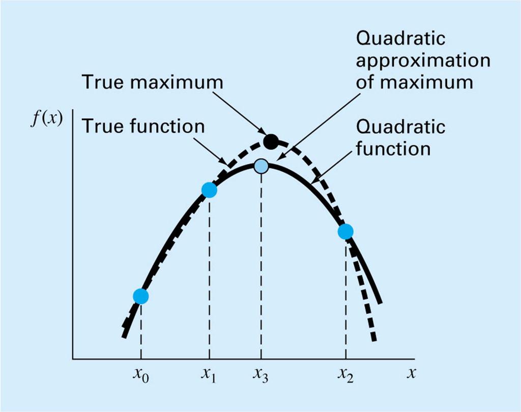
92

93

94

95 x x - rx rx ( x rx) r x 1 r r r r 1 0 r 2 x rx r 2 x r r 2 x r

96 Importance of Number of Function Evaluations In small problems this does not matter Reduced function evaluations means faster performance This matters if a large number of optimizations needs to be performed This matters if one function evaluation is expensive in computation time

97 Error Analysis for Golden Section Search At the end of each iteration, we have an interval that is known to contain the optimum We analyze the case where the left-hand interval is discarded; the other case is symmetric Old points are x l, x 2, x 1, and x u New points are x 2, x 1, and x u, x 1 is guess

98 x x x rx ( x) [ x rx ( x)] 1 2 l u l u u l ( x x ) 2 r( x x ) u l u l (2r 1)( x x ) u l.236( x x ) u l x x x [ x r( x x )] u 1 u l u l (1 r)( x x ) u l.382( x x ) u l

99 Quadratic Interpolation If golden section search is analogous to bisection, then the equivalent of linear interpolation (false position) is quadratic interpolation We approximate the function over the interval by a quadratic (parabola), and solve the quadratic Requires three points instead of two

100 Fig 13.6

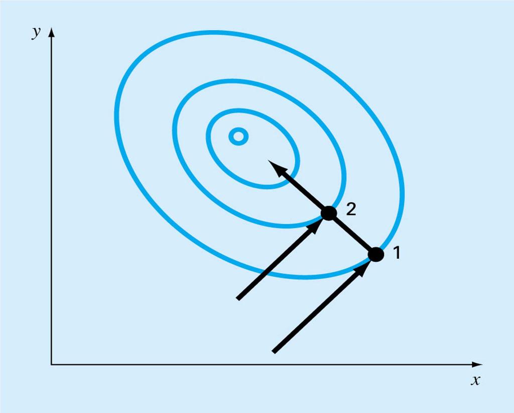
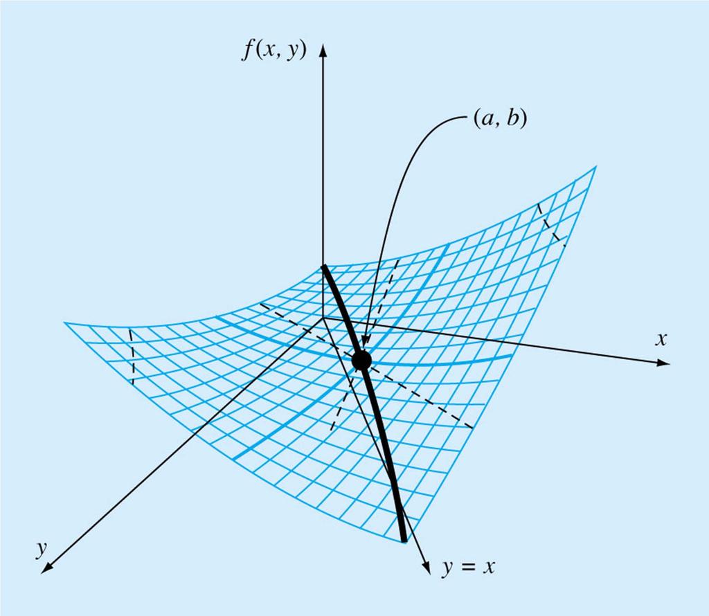
101 Given three points find the quadratic joining them ( x, f( x )) 0 0 ( x, f( x )) 1 1 ( x, f( x )) 2 2 f ( x) ax bx c f ( x ) ax bx c f ( x ) ax bx c f ( x ) ax bx c

102 f( x ) ax bx c f( x ) ax bx c f( x ) ax bx c x x 1 a f( x ) x x 1 b f( x ) x x 1 c f( x )

103 x f( x0)( x1 x2) f( x1)( x2 x0) f( x2)( x0 x1) 2 f( x )( x x ) 2 f( x )( x x ) 2 f( x )( x x ) Initial endpoints are x 0 and x 2 Initial middle point is x 1 New middle point as guess for the optimum is x 3 Discard one of x 0 or x 3 using the same rule as golden section search Error estimate usually by change in estimate

104 Newton s Method Open rather than bracketing method, analogous to Newton-Raphson Also uses a quadratic model of the function Quadratic model is at a point not over an interval Optimum is when the derivative is 0 Use Newton-Raphson on the derivative

105 f ( x) f ( x ) f '( x )( x x ) 0.5 f ''( x )( x x ) f '( x) f '( x ) 0.5 f ''( x )2( x x ) f ''( x )( x x ) f '( x ) 0 f '( x ) f ''( x )( x x ) i i i ( x x ) f '( x ) / f ''( x ) i i i i i i i i i i i i i i x x f '( x ) / f ''( x ) i 1 i i i 2

106 Error behavior of optimization methods in dimension 1 Golden section search has linear convergence with ratio φ and an error bound Quadratic interpolation has linear convergence and an error estimate from change in the estimate Newton s method has quadratic convergence and an error estimate from change in the estimate

107 Pitfalls of Newton s Method Different starting points may lead to different solutions Iterations may diverge The former requires repeated search for the optimal optimum = global optimum The latter may require limiting step size, or requiring an increase in function value at each iteration

108 Multidimensional Unconstrained Optimization Suppose we have a function f() of more than one variable f(x 1, x 2,, x n ) We want to find the values of x 1, x 2,, x n that give f() the largest (or smallest) possible value Graphical solution is not possible, but a graphical picture helps understanding Hilltops and contour maps

109 Methods of solution Direct or non-gradient methods do not require derivatives Grid search Random search One variable at a time Line searches and Powell s method Simplex optimization

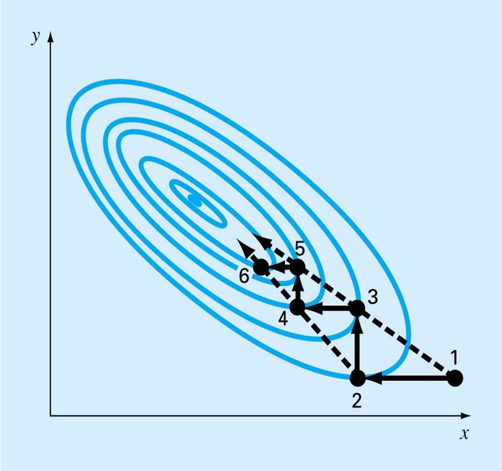
110 Gradient methods use first and possibly second derivatives Gradient is the vector of first partials Hessian is the matrix of second partials Steepest ascent/descent Conjugate gradient Newton s method Quasi-Newton methods

111 Grid and Random Search Given a function and limits on each variable, generate a set of random points in the domain, and eventually choose the one with the largest function value Alternatively, divide the interval on each variable into small segments and check the function for all possible combinations

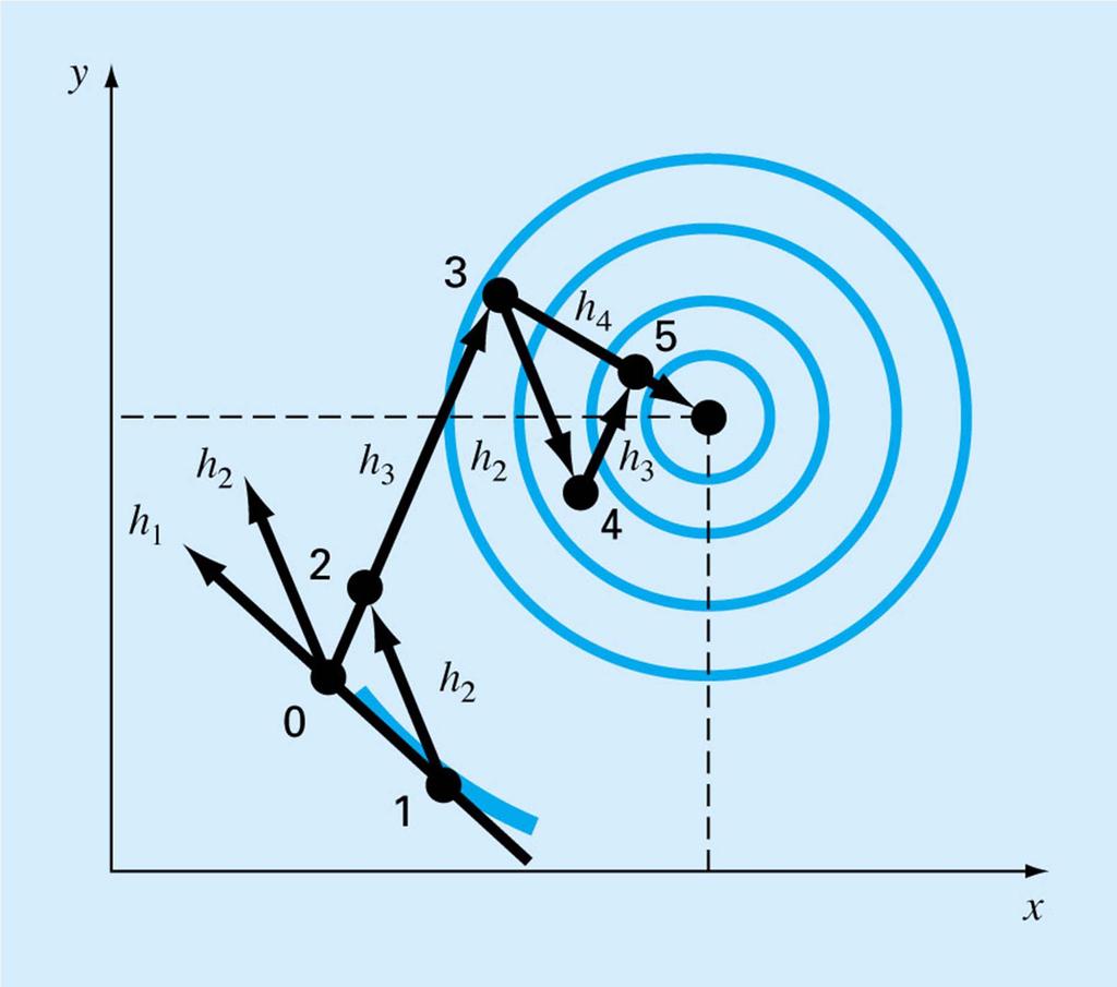
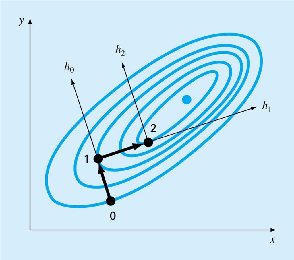
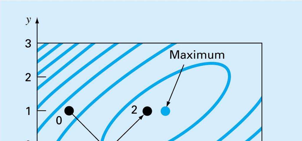
112 Features of Random and Grid Search Slow and inefficient Requires knowledge of domain Works even for discontinuous functions Poor in high dimension Grid search can be used iteratively, with progressively narrowing domains

113 Line searches Given a starting point and a direction, search for the maximum, or for a good next point, in that direction. Equivalent to one dimensional optimization, so can use Newton s method or another method from previous chapter Different methods use different directions

114 x v ( x, x,, x ) 1 2 ( v, v,, v ) 1 2 n n f ( x) f( x, x,, x ) 1 2 g( λ) f ( x λv) n

115 One-Variable-at-a Time Search Given a function f() of n variables, search in the direction in which only variable 1, changes Then search in the direction from that point in which only variable 2 changes, etc. Slow and inefficient in general Can speed up by searching in a direction after n changes (pattern direction)

116

117 Powell s Method If f() is quadratic, and if two points are found by line searches in the same direction from two different starting points, then the line joining the two ending points (a conjugate direction) heads toward the optimum Since many functions we encounter are approximately quadratic near the optimum, this can be effective

118

119 Start with a point x 0 and two random directions h 1 and h 2 Search in the direction of h 1 from x 0 to find a new point x 1 Search in the direction of h 2 from x 1 to find a new point x 2. Let h 3 be the direction joining x 0 to x 2 Search in the direction of h 3 from x 2 to find a new point x 3 Search in the direction of h 2 from x 3 to find a new point x 4 Search in the direction of h 3 from x 4 to find a new point x 5

120 Points x 3 and x 5 have been found by searching in the direction of h 3 from two starting points x 2 and x 4 Call the direction joining x 3 and x 5 h 4 Search in the direction of h 4 from x 5 to find a new point x 6 The new point x 6 will be exactly the optimum if f() is quadratic The iterations can then be repeated Errors estimated by change in x or in f()

121

122 Nelder-Mead Simplex Algorithm Direct search method that uses simplices, which are triangles in dimension 2, pyramids in dimension 3, etc. At each iteration a new point is added usually in the direction of the face of the simplex with largest function values

123

124 Gradient Methods The gradient of f() at a point x is the vector of partial derivatives of the function f() at x For smooth functions, the gradient is zero at an optimum, but may also be zero at a non-optimum The gradient points uphill The gradient is orthogonal to the contour lines of a function at a point

125 Directional Derivatives Given a point x in R n, a unit direction v, and a function f() of n variables, we can define a new function g() of one variable by g(λ)=f(x+λv) The derivative g (λ) is the directional derivative of f() at x in the direction of v This is greatest when v is in the gradient direction

126 x v 1 ( x, x,, x ) 1 2 ( v, v,, v ) T vv 1 2 i 1 2 i f( x) f( x, x,, x ) 1 2 f f f f,,, x x x 1 2 g( λ) f ( x λv) n v n n n T f f f g'(0) ( f) v v, v,, vn x x x n n

127 Steepest Ascent The gradient direction is the direction of steepest ascent, but not necessarily the direction leading directly to the summit We can search along the direction of steepest ascent until a maximum is reached Then we can search again from a new steepest ascent direction

128 x x f( x, x ) at (2,2) f (2,2) f ( x, x ) x f (2,2) 4 f ( x, x ) 2 x x f (2,2) f (2,2) (4,8) (2 4 λ,2 8 λ) is the gradient line g( λ) f (2 4 λ,2 8 λ) (2 4 λ)(2 8 λ) 2

129

130

131 The Hessian The Hessian of a function f() is the matrix of second partial derivatives The gradient is always 0 at a maximum (for smooth functions) The gradient is also 0 at a minimum The gradient is also 0 at a saddle point, which is neither a maximum nor a minimum A saddle point is a max in at least one direction and a min in at least one direction

132

133 Max, Min, and Saddle Point For one-variable functions, the second derivative is negative at a maximum and positive at a minimum For functions of more than one variable, a zero of the gradient is a max if the second directional derivative is negative for every direction and is a min if the second directional derivative is positive for every direction

134 Positive Definiteness A matrix H is positive definite if x T Hx > 0 for every vector x Equivalently, every eigenvalue of H is positive λ is an eigenvalue of H with eigenvector x if Hx = λx -H is positive definite if every eigenvalue of H is negative

135 Max, Min, and Saddle Point If the gradient f of a function f is zero at a point x and the Hessian H is positive definite at that point, then x is a local min If f is zero at a point x and -H is positive definite at that point, then x is a local max If f is zero at a point x and neither H nor -H is positive definite at that point, then x is a saddle point The determinant H helps only in dimension 1 or 2

136 Finite-Difference Approximations If analytical derivatives cannot be evaluated, one can use finite-difference approximations Centered difference approximations are in general more accurate, though requiring extra function evaluations Increment often macheps 1/2 or 1e-8 for dp This can be problematic for large problems

137 Complexity of Finite-Difference Derivatives In an n-variable problem, the function value is one function evaluation (FE) A finite-difference gradient is n FE s if forward or backward and 2n FE s if centered. A finite difference Hessian is O(n 2 ) FE s With a thousand variable problem, this can be huge

138 Steepest Ascent/Descent This is the simplest of the gradient-based methods From the current guess, compute the gradient Search along the gradient direction until a local max is reached of this onedimensional function Repeat until convergence

139

140 f( x, x ) 2x x 2x x 2x f x f x ( x, x ) f ( x, x ) 2x 2 2x ( x, x ) f ( x, x ) 2x 4x True optimum 0 2x 2 2x x 4x x ( x, x ) (2,1) 2 2 H 2 4 2

141 Eigenvalues If H is a matrix, we can find the eigenvalues in a number of ways We will examine numerical methods for this later, but there is an algebraic method for small matrices We illustrate this for the Hessian in this example

142 H Hx H I x x ( 2)( 4) x 0 2 solution is a maximum

143 f x f x f( x, x ) 2x x 2x x 2x ( x, x ) f ( x, x ) 2x 2 2x ( x, x ) f ( x, x ) 2x 4x f ( 1,1) 7 f ( 1,1) 2x 2 2x f ( 1,1) 2x 4x g( ) f( 1 6,1 6 )

144 g( ) f( 1 6,1 6 ) 2( 1 6 )(1 6 ) 2( 1 6 ) ( 1 6 ) 2(1 6 ) g '( ) x ( 1 6(.2),1 6(.2)) (.2,.2) 2 2

145 f (2,1) 2 f (1, 1) 7 f (0.2, 0.2) 0.2 f f 1 2 (0.2, 0.2) 1.2 (0.2, 0.2) 1.2 g( ) f( , ) g '( ) f (1.4,1) 1.64

146

147 Practical Steepest Ascent In real examples, the maximum in the gradient direction cannot be calculated analytically Problem reduces to one dimensional optimization as a line search One can also use more primitive line searches that are fast but do not try to find the absolute optimum

148 Newton s Method Steepest ascent can be quite slow Newton s method is faster, though it requires evaluation of the Hessian Function is modeled by a quadratic at a point using first and second derivatives The quadratic is solved exactly This is used as the next iterate

149 A second-order multivariate Taylor series expansion at the current iterate is T T f( x) f( x ) f ( x )( x x ) 0.5( x x ) H ( x x ) i i i i i i At the optimum, the gradient is 0, so f( x) f( x ) H ( x x ) 0 i i i If H is invertible,then 1 x i 1 x i H i f( xi) In practice, solve the linear problem, H x H x f( x ) i i i i