EXPERIMENTAL MEASUREMENT OF RADIATION HEAT TRANSFER FROM COMPLEX FENESTRATION SYSTEMS

Transcription

1 EXPERIMENTAL MEASUREMENT OF RADIATION HEAT TRANSFER FROM COMPLEX FENESTRATION SYSTEMS By BARRY ALLAN WILSON Bachelor of Science Oklahoma State University Stillwater, Oklahoma 2005 Submitted to the Faculty of the Graduate College of the Oklahoma State University in partial fulfillment of the requirements for the Degree of MASTER OF SCIENCE May, 2007

2 EXPERIMENTAL MEASUREMENT OF RADIATION HEAT TRANSFER FROM COMPLEX FENESTRATION SYSTEMS Thesis Approved: Dr. Dan Fisher Thesis Adviser Dr. Jeffrey Spitler Dr. Lorenzo Cremaschi Dr. A. Gordon Emslie Dean of the Graduate College ii

3 ACKNOWLEDGEMENTS First, I would like to recognize my late father Ted Wilson and late grandparents Webster and Lois Allan, who taught me to set lofty goals and always give my best. And although your lives were not long enough to see this day, it has been my constant drive to make you proud that has gotten me where I am today. I would like to give my sincere gratitude for my advisor Dr. Dan Fisher, whose overly optimistic attitude and extreme accessibility made every problem seem surmountable. His continuous advice and guidance was extremely helpful through this process, I only wish I would have listened to it more often. I would also like to thank my committee members Dr. Jeffrey Spitler and Dr. Lorenzo Cremaschi for their guidance on my work. I would also like to thank my friends in the BACTL, Chanvit Chantrasrisalai, Chris Carroll and Sankaranarayanan Padhmanabhan, without their continued help this thesis truly would not have been possible. Kyong Edwards, John Gage and Jerry Dale also provided their time and many talents through the course of this project. I would like to recognize my colleagues in ATRC 337, ERL 110 and in my courses for providing their advice, help and friendship. I have always been a believer in the old proverb We have no friends, We have no enemies, We have only teachers. Therefore, I would like to take this opportunity to thank some of the great teachers in my life: Matt Youngblood, Brent Wilson, Phillip iii

4 White, Colin Eddy, Bob and Kris Richey, John and Carmen Rutherford, Frank and Sheri Capps, Penny Crofford, Sherry Bass and Carrie Witham. I would also like to thank my entire family, who are always willing to give advice and time whenever I am in need, and my beautiful wife Jennifer for her constant encouragement and understanding through this process. Finally, I would like to thank the one person I have always admired and respected the most, my mother Susan Wilson, who through immense adversity taught me every lesson I have ever truly needed to know. From the time I was a little kid I have hoped to one day be as intelligent and as good of a person as you are, unfortunately I still have a long way to go. iv

5 TABLE OF CONTENTS Chapter Page Nomenclature... xi English Letter Symbols... xi Greek Letter Symbols...xiii 1 Introduction Background Significance Thesis Scope Literature Review LBNL (Klems) Experiments at Queen s & Ryerson Polytechnic Universities Laboratory Studies Calorimetric Studies Description of Experimental Facility Overall Design and Capabilities Room Configuration Heated Window Panel Heated Blinds Calculations, Instrumentation and Experimental Uncertainty Calculations Heat Balance Calculations Convective/Radiative Split Calculations Convection Coefficient Calculations Thermal Conductance Calculations Calculation of Experimental Uncertainties Primary Measurements and Uncertainty Data Acquisition Unit Temperature Measurements Room Surfaces Window Surface Window Guard Panel Blinds Air Guard Space Power Measurements Radiant Heat Flux Pressure Airflow Speed v

6 4.3 Uncertainties in Intermediate Variables Room Airflow Rate Heat Extraction Rate Radiant Heat Gains Total Fenestration Heat Gain Convective Heat Gain Fictitious Fenestration Surface Temperature Propagation of Uncertainty Analysis to Results Radiative/Convective Split Convection Coefficient Thermal Conductance Validation of Experimental Facility Experimental Procedure Test Procedure Parametric Simulation Set Results Flow Field Analysis Heat Transfer Analysis Assessment of the Facility and Experimental Procedure Conclusions Assessment of the Results Future Work and Recommendations Facility Instrumentation References Appendix A: Standard Operating Procedures Appendix B: Maintenance Procedures Appendix C: Troubleshooting Appendix D: Facility Pictures Appendix E: Thermocouple Calibration Summary Appendix F: DAQ Unit Channels Appendix G: Computer Control Board Channels Appendix H: HVAC System Diagrams vi

7 LIST OF TABLES Table 2-1 Final results from Machin et al (1998) Table 2-2 Final results from Duarte et al (2001) Table 5-1 Parameters for the 52 experiments Table 6-1 Radiative fractions, uncertainty and parameters for each test Table E-1 Thermocouple calibration summary (Chantrasrisalai 2007b) Table F-1 Fluke channel configuration (Chantrasrisalai 2007b) Table G-1 DAC channel diagram (Chantrasrisalai 2007b) Table G-2 DAS channel layout (Chantrasrisalai 2007b) Note the safety board channels are in identical order as channels vii

8 LIST OF FIGURES Figure 1-1 Illustration of the combined fictitious layer assumption... 3 Figure 2-1 Sketch of the experimental model at Queen s University (Machin et al. 1998)8 Figure 3-1 Isometric sketch of Building Airflow and Contaminant Transport Test Rooms (Fisher and Chantrasrisalai 2006) Figure 3-2 Elevation view of the air handling system (Fisher and Chantrasrisalai 2006) 16 Figure 3-3 Layout view of the modified lower zone Figure 3-4 Side view of the window enclosure design Figure 3-5 Ceiling/Airflow configuration # Figure 3-6 Ceiling/Airflow configuration # Figure 3-7 Construction of heated window panel system Figure 4-1 Location of thermocouples on the window panel Figure 4-2 Traversing mechanism used for net radiation and airspeed measurements Figure 4-3 Sensitivity of the radiant gain to measurement grid density (Chantrasrisalai 2007b) Figure 4-4 Validation of measured radiant heat gain (Chantrasrisalai 2007a) Figure 4-5 Validation of calculated window surface temperature (Chantrasrisalai 2007a) Figure 4-6 Repeatability of the radiant fraction Figure 4-7 Repeatability of the equivalent convection coefficient (based on supply air temperature) viii

9 Figure 5-1 Illustration of the three different gap-widths, from left to right 0.5 in. (12.7 mm), 1.75 in. (44.5 mm) and 3.75 in. (95.25 mm) Figure 5-2 Illustration of the three different blind slat angles, from left to right -45, 0º and Figure 6-1 Airspeed [ft/min] distribution in front of and immediately above the fenestration system for zero system airflow Figure 6-2 Temperature profile of fenestration system with zero system airflow Figure 6-3 Airspeed [ft/min] distribution for 5 ACH from radial diffuser, no fenestration power dissipation Figure 6-4 Airspeed [ft/min] distribution for 10 ACH from radial diffuser, no fenestration power dissipation Figure 6-5 Airspeed [ft/min] distribution for 5 ACH from linear slot diffuser Figure 6-6 Temperature profile of fenestration system for 5 ACH from linear slot diffuser Figure 6-7 Airspeed [ft/min] distribution for 10 ACH from linear slot diffuser Figure 6-8 Temperature profile of fenestration system for 10 ACH from linear slot diffuser Figure 6-9 Sketch of the wall jet separation point Figure 6-10 Effect of various parameters on radiant fraction, high power = 150W, low power = 50W from each fenestration component Figure 6-11 Effect of component power dissipation on the radiant fraction for different slat angles and system airflow rates ix

10 Figure 6-12 Radiative fraction for various slat angles and airflow configurations with a gap width of 0.5 in Figure 6-13 Radiative fraction for various gap widths and airflow configurations Figure D-1 Tank fill/drain line filters and valves Figure D-2 Tank side of the fill/drain line Figure D-3 Air filter housing before main cooling coil Figure D-4 Air filter housing on third level Figure D-5 Variable transformer bank Figure D-6 Cooling coil condensate drain fill pipe Figure D-7 Safety boards Figure D-8 Location of the master relay Figure D-9 Rack mount Figure H-1 System diagram for the NE fan coil unit loop (Chantrasrisalai 2007b) Figure H-2 System diagram for the SW fan coil unit loop (Chantrasrisalai 2007b) Figure H-3 System diagram for the air handler unit loop (Chantrasrisalai 2007b) Figure H-4 System diagram for the heat pump loops (Chantrasrisalai 2007b) x

11 Nomenclature English Letter Symbols A A1 ACH cl cl+1 C p DAQ E b, j F k Area Plane area of the fenestration system Room air changes per hour Thermal conductance of innermost glazing layer Thermal conductance of the fictitious layer Specific heat of air Data acquisition unit Black-body emissive power of the surface j 1 View factor from the fictitious surface to the room surface k F, Fraction of fenestration heat gain transferred through convection fen conv F fen, Fraction of fenestration heat gain transferred through thermal rad radiation F j k View factor from surface j to surface k FS Full-scale h fen Fenestration convection coefficient HVAC Heating, Ventilation and Air conditioning system J Radiosity m& a Mass flow rate of air Q Room volumetric flow rate q& cond q& & error q fen, tot q & fen, rad q& plug q & rad, i q& space q& wd T T T 1 ra ref Conduction heat loss through zone surfaces Heat balance error Power input to the fenestration system Total radiative heat transfer rate from fenestration system Power input to the plug load Net radiative heat flux at a given measurement location Zone heat extraction rate Power dissipated by the heat window panel Temperature of the fictitious fenestration surface temperature Temperature of air at the return grill Reference air temperature xi

12 Tsa surf in Temperature of air at the supply diffuser T, Temperature of the inside surface T, Temperature of the outside (guard space side) surface surf out Twd U u u u A c f Temperature of the innermost glazing layer Estimated overall heat transfer coefficient of surface Uncertainty in flow nozzle area Uncertainty in flow nozzle discharge coefficient Uncertainty in differential pressure measurement u F fen, Uncertainty in the convective fraction conv Uncertainty in the radiative fraction u F fen, rad um u m, i u N u Q u q& bl, inp Total uncertainty in primary measurements Uncertainty caused by individual sources Uncertainty caused by variations in the fan speed Total uncertainty in airflow rate Uncertainty in blind power dissipation u q & Uncertainty in T 1 due to the uncertainty in the net radiant heat gain u q & cond u q & ext u q& fen, conv u q& fen, rad u q& fen, tot u q & rad u q rad, i Uncertainty in conduction heat transfer rate Uncertainty in heat extraction rate Uncertainty in the convective heat gain Uncertainty in radiant heat gain from the fenestration system Uncertainty in total fenestration heat gain Uncertainty in net radiant heat gain Uncertainty in net radiant heat flux u q& wd, inp Uncertainty in window panel power dissipation ut Uncertainty in 1 ut 1 u TT n utε 1 u y u T cond u T ext T due to the uncertainty in the room surface temperatures Uncertainty in the fictitious fenestration surface temperature Uncertainty of the surface temperature of the n th room surface Uncertainty due to the propagation of the uncertainty of the emissivity of the fictitious surface Uncertainty in derived variable Uncertainty in the difference between inside surface temperature and guard space air temperature Uncertainty in temperature difference uε Uncertainty in T 1 due to the uncertainty in the room surface xii

13 uε 1 u ρ emissivities Uncertainty in the emissivity of the fictitious surface Uncertainty in air density Greek Letter Symbols T ext T T ε j σ fen ref fen wd Difference between entering and leaving air temperatures Difference between fictitious surface temperature and the reference Difference between fictitious surface temperature and the temperature of the window panel Emissivity of the inside surface j Stefan-Boltzmann constant xiii

14 1 Introduction 1.1 Background Significance Venetian blinds are a very common window-shading device to provide privacy and daylighting control; they can be found in the majority of households and many commercial buildings. Although Venetian blinds are a very common device, their effect on cooling and heating loads is very complicated and is not currently completely understood. The complications come from the fact that the blinds themselves are partially specular and partially diffuse in the visible spectrum and affect the local airflow differently depending on the absorbed solar radiation. Furthermore, these effects can be modified at any time by the user. Due to these complexities Venetian blinds are likely the most common building envelope element that does not have a suitable simulation model. Although several simulation models have been proposed in the literature (Klems 1994a; 1994b; Klems et al. 1995b; Ye et al. 1999; Phillips et al. 2001; Naylor et al. 2002; Naylor et al. 2006; DOE 2007), they have all been hampered by the lack of experimental investigations into their required parameters. The experiments that have been performed have been very complex and expensive to run resulting in little usable data. The previous experiments were also conducted with only buoyancy driven airflows and the experimental setup was isolated from all other airflows. Since only natural convection was considered in previous experimental studies, it is likely that their results are 1

15 unrealistic due to the fact that blinds in conditioned zones are usually exposed to either wall jets or free jets. Due to the continued tightening of energy standards such as ASHRAE s Standard 90.1, the desire for accurate energy simulations has increased in recent years. In order to meet this desire, Chantrasrisalai (2007a) recently developed a new model to describe Venetian blinds. The Chantrasrisalai model proposed that the innermost glazing surface and the blinds be modeled as one fictitious layer. This fictitious layer consists of two sublayers; the back sublayer is the (real) innermost glazing while the front sublayer is comprised of the blinds and the air gap between the two real layers as illustrated in Figure 1-1. It is further assumed that the two sublayers are in perfect thermal contact and the layer has a thermal conductance of c L+ 1, which must be found experimentally. Utilizing the fictitious layer simplification, it was possible to develop a straightforward experimental method to determine the heat transfer coefficients and radiative-convective splits needed for radiant time series (RTS) and heat balance (HBM) load calculation methods. The complete description, development and usage of the model can be found in the literature (Chantrasrisalai 2007a). 2

16 Figure 1-1 Illustration of the combined fictitious layer assumption 1.2 Thesis Scope The scope of the current thesis was to develop and validate a facility to conduct the experimental method proposed by Chantrasrisalai and to perform a limited parametric set of experiments. The facility was built inside Oklahoma State University s Building Airflow and Contamination Transport Laboratory. The facility, described in detail in Chapter 3, required many modifications and additions to the laboratory. Some of these modifications include: Construction of electrically-heated window blinds and window panel system to simulate the heating of an actual fenestration system from absorbed solar radiation. Construction of a partition wall and window enclosure that could handle multiple configurations of the window-blind system. 3

17 Addition of wall paneling to provide uniform wall surfaces, including texture and optical properties. Addition of new instrumentation. The parametric set included 52 experimental tests, not including validation and sensitivity tests. Several variables including the slat angle, room airflow rate, blind and window panel heat fluxes, window-blind gap width and airflow configuration were varied in the set of experiments. Results were used to show the differences with respect to the natural convection assumption utilized in several previous studies. 4

18 2 Literature Review Although there has been a great deal of theoretical and numerical research into the effects of complex fenestration systems (Klems 1994a; 1994b; Klems et al. 1995b; Ye et al. 1999; Oh et al. 2001; Phillips et al. 2001; Naylor et al. 2002; 2006), there has been very little recent experimental work on the subject. All of the recent experimental research was conducted at Lawrence Berkeley Nation Laboratory (LBNL) and a group of Canadian universities including Queen s, Ryerson Polytechnic and Waterloo. Although the researchers produced reasonable and consistent results, they all made a major assumption that convection was driven by buoyancy effects only. This assumption is likely to be unrealistic considering that a shading layer in an actual building will be exposed to air currents and many are adjacent to slot diffusers. The experimental work of these two groups will be analyzed in detail in the following sections. 2.1 LBNL (Klems) In the mid-1990s, Klems et al. developed a model to predict the effects of shading on solar heat gains. The model was based on two concepts: First, the optical properties of the system were considered a function of the optical properties of each glazing or shading layer. Second, the inward flowing fraction was considered solely a thermal property of each layer independently of the layer s optical properties (Klems 1994a; 1994b; Klems et al. 1995b). 5

19 Experimental research at LBNL supported their model and provided reference data suitable for a handbook. In 1995, Klems and Warner published a paper detailing a method to determine the bidirectional optical properties of shading devices utilizing a scanning radiometer. They validated their method by determining the optical properties of a Venetian blind, one of the most optically complex shading devices available, and showed their method was significantly quicker than calorimetric measurements (Klems and Warner 1995a). In 1996, Klems and Kelley produced a method for determining the inward-flowing fraction through calorimetric studies. By utilizing a dual chamber calorimeter where both chambers had an identical setup, they were able to determine the shading layer s specific inward-flowing fraction by slightly heating the shading device in one chamber. Using this method they found the inward flowing fraction for a limited set of configurations (Klems and Kelley 1996). A correlation for the inward-flowing fraction was later developed for Venetian blinds (Collins and Harrison 1999). The results of the previous two papers were brought together in 1997 to show the utility of the model the researchers had developed. They determined that the model, with the experimental results, provided a reasonable picture of the performance of a complex fenestration system (Klems and Warner 1997). However, this model has not been widely used because of the lack of a database containing the optical and thermal properties of various shading layers. 6

20 2.2 Experiments at Queen s & Ryerson Polytechnic Universities Laboratory Studies At Queen s and Ryerson Polytechnic Universities in Ontario, Canada, work has centered on modeling heat transfer from the blinds using finite element methods. Both research groups experimentally validated their models. The facility at Queen s consisted of a Venetian blind placed in front of a vertical plate that represented the inner pane of a fenestration system. A sketch of the facility is shown in Figure 2-1. In earlier studies the vertical panel was heated with electrical strip heaters, while later studies heated and cooled the panel utilizing hydraulic flow channels (Machin et al. 1998; Collins et al. 2001). The plate was precision ground and had a beveled bottom edge to promote ideal boundary layer formation (Machin et al. 1998). Temperature within the plate was measured with ten 24-gauge copper-constantan thermocouples, and one platinum RTD sensor that were placed in holes drilled on the backside of the plate to within.08in (2mm) of the surface. The leading edge temperature was measured with one 40-gauge thermocouple placed 0.20in (5mm) from the tip (Machin et al. 1998). The Venetian blinds also matured in later studies, the original setup utilized unheated blind slats while later studies heated the slats with two foil heating strips bonded to the concave surface of the slats (Machin et al. 1998; Collins et al. 2001). In all experiments the slats were taken from a commercially available aluminum Venetian blind set. The emissivity of the slats and vertical plate were modified for the given experiments. To allow for interferometer measurements an optical window constructed from plexiglass was placed on either side of the setup. The setup was also covered in a large 7

21 tent designed to reduce the effect of air circulation in the room (Machin et al. 1998). This tent also ensured that only natural convection would occur. Figure 2-1 Sketch of the experimental model at Queen s University (Machin et al. 1998) The first experiments at this facility were performed by Machin et al. They wanted to determine the influence of a Venetian blind on the average and local natural convection coefficient. Their results were intended to validate a finite element analysis program that was being developed by the authors. This program would later be used to conduct a full parametric study including secondary parameters, such as blind width and conductivity. Between each experiment, the aluminum plate was polished to give it an emissivity between 0.04 and The plate was also heated to 36 F (20 C) above ambient and was isothermal to within 0.65 F (0.36 C). The blinds for this set of experiments were unheated with a hemispherical emissivity of ±0.02. Temperature measurements were conducted with a Mach-Zehnder Interferometer, while flow visualizations were produced by reflecting laser light off cigarette smoke. Experiments were conducted for 8

22 blind angles of -45, 0, 45 and 90 and gap widths of 0.51in, 0.57in and 0.59in (13 mm, 14.5 mm, 17 mm) (1998). Machin et al. validated their experiments against theoretical correlations for natural convection on a vertical plate produced by Ostrach (1953); this validation was performed with only the vertical plate installed without the presence of the blinds (1998). The average convection coefficient found by the validation was approximately 3% higher than theoretical, which was within the experimental uncertainty of 4% (Machin et al. 1998). It was found that the blind had very little influence at a gap width of 0.59in (17mm), but it had strong influence at narrower gap widths. Blind angle was also shown to have a large influence on the temperature distribution. Even though the blinds had a large effect on the temperature distribution, the local convection coefficients showed similar trends with and without the blind, decaying rapidly from the leading edge. The blinds did, however, cause strong periodic spikes, the amplitude of which was dependent on the distance between the blind tips and the vertical plate. Their final results showed that the average convection coefficient was reduced for all cases except the fully closed and the horizontal test with the minimum gap width (Machin et al. 1998). The final results of their experiment can be seen in Table 2-1. Although this research found heat transfer coefficients on the innermost glazing of a complex fenestration system, it should be noted that the test conditions were not completely realistic. The results were produced without a heated blind and neglected the effects of impinging wall and free jets from nearby diffusers, both of which would be present in a real fenestration system. It is also believed that a wider gap width should have been investigated, considering the many Venetian 9

23 blinds are installed flush with the wall surface, which can be many inches from the glazing system. Table 2-1 Final results from Machin et al (1998) The next set of experiments performed at this facility was conducted by Duarte et al. For this set of experiments the vertical panel and blinds were painted to give a hemispherical emissivity of 0.81 ±0.02. They performed 18 experiments with the following parameters: gap widths of 0.57in and 0.59in (14.5mm, 17.0mm), blind slat angle of -45, 0 and 45 and blind heat fluxes of 0, 0.26 and 0.77 BTU/hr-in 2 (0, 120, 350 W/m 2 ). The vertical plate was kept at 27 F (15 C) above ambient and was isothermal to within 0.72 F (0.4 C) (Duarte et al. 2001). Duarte et al also noticed the strong periodic increase in local convection coefficient near the tips of the blind slats. They showed that the convection coefficient from the panel decreased drastically with an increase in blind flux (2001). Their final results can be seen in Table 2-2, it should be remembered that the convection coefficients shown are from the vertical panel, not from the entire system to the zone. As with the test conducted by Machin et al (1998) this test did not include the effects of mechanically driven jets and covered a very limited range of gap widths. The vertical panel convection coefficients are of limited usefulness, they do not show how the entire system interacts with the zone. 10

24 Table 2-2 Final results from Duarte et al (2001) Collins et al conducted the next set of experiments in the facility. The purpose of his experiments was to validate a finite element program the authors had developed. Part of the validation included a cool vertical panel; therefore the heating strips on the panel were replaced with the flow channel arrangement previously discussed. A total of eight experiments were conducted with three different slat angles -45, 0 and 45, two gap widths 0.61in and 0.79in (15.4mm, 20mm), two blind heat fluxes and 0.33 BTU/hrin 2 (125 and 150 W/m 2 ) and two plate temperatures F and 1.8 F (-14 C, 1 C) relative to ambient (Collins et al. 2001). Although they did not present actual convection coefficients, only temperatures and fluxes, it could be seen in the data that blind slat angle had little effect at the larger gap width but the gap width had significant influence (Collins et al. 2001). Only one slat angle (0 ) was tested for the shorter gap width, but results for a warm panel and short gap width were found by Duarte et al as previously discussed (2001). The full validation of the authors finite element model was reported in another paper (Collins et al. 2002) Calorimetric Studies The ultimate goal of the researchers at Queen s, Ryerson and Waterloo Universities was to upgrade window analysis software to include the effect of interior shading devices (Collins and Harrison 2004). In order to validate this software, full scale tests were 11

25 performed utilizing a solar calorimeter located at Queen s University. Twelve tests were performed with one glazing system, two sets of blinds, three blind angles -45, 0 and 45 and two solar profile angles of 30 and 45. The two sets of blinds were identical except for their color; one was painted with white enamel while the other was painted flat black. The white and black blinds had solar absorptances of 0.32 and 0.90 and hemispherical emissivities of 0.75 and 0.89, respectively (Collins and Harrison 2004). Due to weather conditions and the relatively short period of the year appropriate for solar calorimetric studies, two test configurations were not tested by Collins and Harrison. It should be noted that multiple test runs were conducted and averaged to produce the final results. They determined that the presence of the Venetian blinds did not significantly affect the thermal transmission (U-factor) of the glazing systems. It did, however, have a large impact on the solar heat gain. The black blind reduced the solar heat gain by 5% to 10%, with the largest occurring when the blind intercepted the majority of the solar radiation. The more reflective white blind reduced the solar heat gain by 9% to 37%. When the blinds were set to reflect the majority of the solar radiation there was a 37% reduction in the heat gain, the blinds at 0 achieved a 19% reduction, even when the blinds were turned to allow in as much solar radiation as possible they still provided a reduction of 9% (Collins and Harrison 2004). Although the researcher produced impressive results, their experimental method still has some flaws. First, a calorimeter has no mechanically driven airflows, thus only natural convection occurred. Real conditions usually expose complex fenestration systems to air currents, which could drastically increase the convection rates. Second, the 12

26 experimental method would be very expensive and time consuming to implement on the scale required to produce empirical heat transfer correlations. 13

27 3 Description of Experimental Facility The experimental studies for the current thesis were performed in the Building Airflow and Contaminant Transport Laboratory at Oklahoma State University. The experimental facility configuration and equipment are described in the following sections. 3.1 Overall Design and Capabilities The experimental facility consisted of two large office sized rooms with a connecting stairwell as shown in Figure 3-1. The test rooms were located inside a large three-story laboratory. Although upper and lower zones are identical in size and construction, except the upper zone only has one entry door, only the lower zone was utilized for the current research project. Each zone had a commercially available raised flooring system as well as a standard suspended ceiling. During tests the space surrounding the lower zone as well as the upper and lower floor plenums were used as temperature controlled guard spaces. These guard spaces are controlled to match the temperature within the lower zone to prevent conduction heat transfer through the zone walls. To prevent air leakage during experiments the lower zone was completely sealed using DOW s Seal n Peel caulk. The upper and lower zones were separated by 22-gauge roof decking and 3/4in (19mm) of spray foam. The R-value for the floor construction was estimated to be 5.0 Fft²-hr/Btu (0.9m²-K/W) (ASHRAE 2005). The zone walls were constructed out of 2.69in 14

28 (68.3mm) extruded polystyrene sandwiched between two sheets of hard wall panel. The wall construction had an approximate R-Value of 11.3 F-ft²-hr/Btu (2.0m²-K/W) (ASHRAE 2005). The raised floor tiles were constructed out of steel clad, 1in (25.4mm) thick OSB board. The floors were covered with linoleum tile and 1/8in (3.2mm) thick wall board. The final construction had an approximate R-value of 2.4 F-ft²-hr/Btu (0.4m²-K/W) (ASHRAE 2005). For the current research the standard acoustic ceiling tiles were replaced with 1/8in (3.2mm) thick wall boards with an approximate R-value of 0.18 F-ft²-hr/Btu (0.03m²-K/W) (ASHRAE 2005). Figure 3-1 Isometric sketch of Building Airflow and Contaminant Transport Test Rooms (Fisher and Chantrasrisalai 2006) 15

29 The test room was conditioned by a system that contained variable speed supply and return fans, a mixing box, heating and cooling coils and three ASHRAE Standard flow measurement boxes. An elevation view of the air handling system is shown in Figure 3-2. Although the current project utilized zero outside air, the system was capable of running up to 100% outside air. To allow for parametric studies the system was designed for quick configuration of supply and return ducts/plenums. The facility could run either ducted or plenum supplies and returns. Detailed system schematics are presented in Appendix H. Figure 3-2 Elevation view of the air handling system (Fisher and Chantrasrisalai 2006) 16

30 The guard space was conditioned with two fan-coil units. The fan-coil units were located in the North East corner and the South West corner of the guard space and blew along the North and South walls, respectively. A fan was placed in each of the two remaining corners in order to ensure a uniform temperature in the guard space. The upper and lower floor plenums were supplied conditioned air from the main guard space. The floor plenum supply fans also had an electric reheat coil to help maintain a proper guard temperature. 3.2 Room Configuration As previously mentioned the current project was conducted solely in the lower zone, which was specifically configured for the project as shown in Figure 3-3. The largest modification to the lower zone was the addition of a partition wall. This wall separated the zone into two spaces, the larger of which became the test zone while the smaller became a guard space. A window enclosure was framed into the center of the partition wall; it was designed so that the gap between the heated panel, which simulated the window glazing, and the blinds could range between 0 and 5in (130mm). A side view of the window enclosure design is shown in Figure 3-4. The south entrance door was also removed to allow the inner guard space to mix with the outer guard space. The partition wall and access door were sheathed with 1/8in (3.2mm) wall board painted with Sherwin Williams Eggshell interior latex with a known emissivity of 0.9 ±0.05. The sheathing was backed with 1in (25.4mm) thick DOW blueboard insulation for an approximate R-value of 5.2 F-ft²-hr/Btu (0.92m²-K/W) (ASHRAE 2005). The sides and top of the window enclosure were framed out of 1/2in (12.7mm) thick plexiglass backed with 1in (25.4mm) thick blueboard insulation resulting in an estimated 17

31 R-value of 7.3 F-ft²-hr/Btu (1.29m²-K/W) (ASHRAE 2005). The bottom of the window frame was constructed with a 1in (25.4mm) thick layer of blueboard insulation on top of a Douglas Fir 2x8, which had an approximate combined R-value of 6.5 F-ft²-hr/Btu (1.15m²-K/W) (ASHRAE 2005). The partition wall, access door and window assembly were completely sealed before the start of any test to prevent air leakage from the test zone. Figure 3-3 Layout view of the modified lower zone 18

32 Figure 3-4 Side view of the window enclosure design The current research used two ceiling/airflow configurations. The first configuration, shown as Figure 3-5, used a radial supply diffuser placed in the Northeast corner of the room. The configuration also utilized an unducted return. The second configuration, shown as Figure 3-6, used a four foot long linear slot supply diffuser with two 1/2in (12.7mm) slots placed directly above the fenestration system. For the second configuration, the return grille was moved to the Northeast corner and was ducted. 19

33 Figure 3-5 Ceiling/Airflow configuration #1 The commercial acoustic ceiling tiles in the test zone were replaced with 1/8in (0.32mm) thick wallboard, which had a R-value of 0.2 F-ft²-hr/Btu (0.04m²-K/W) (ASHRAE 2005). The ceiling tiles were painted with the same paint as the other room surfaces. The ceiling tiles over the inner guard space were manufactured out of blueboard insulation with an R-value of 5 F-ft²-hr/Btu (0.88m²-K/W) (ASHRAE 2005). All ceiling tiles were sealed to prevent air leakage to the plenum. The lights were service lights only and were turned off during experiments. For each of the two airflow configurations an electric heater was also placed on the floor in the Northeast corner of the room to simulate realistic plug loads in the space. 20

34 Figure 3-6 Ceiling/Airflow configuration #2 3.3 Heated Window Panel The simulated window consisted of two electric resistance heating panels isolated by 2 inches (0.051m) of DOW blueboard insulation as shown in Figure 3-7. The inside facing panel simulates the innermost glazing layer of a real fenestration system, while the outside facing panel acts as a guard. The completed system was 36in (0.914m) wide by 36in (0.914m) tall by 4.125in (0.105m) deep. 21

35 Figure 3-7 Construction of heated window panel system The two heating panels were identical in construction. The panels had an aluminum heating element, which was backed by 1/2in (0.013m) thick fiberglass insulation. The fiberglass backing had an R-value of 1.86 F-ft²-hr/Btu (0.33m²-K/W) (ASHRAE 2005). Each panel has a rated power output of 450W at 120V thus the resistance can be calculated as 32Ω (SSHC 2003). The panels were powered by two separate variable transformers capable of supplying between 0 and 130V, thus providing a power range of 0 to 528W. The two sheets of blueboard insulation sandwiched between the panels provided resistance to heat transfer allowing the window panel to be more easily guarded. The insulation layer had an overall R-value of 10 F-ft²-hr/Btu (1.76m²-K/W) (ASHRAE 2005). Combined with the fiberglass backing on the heated panels the overall R-Value between heating elements was F-ft²-hr/Btu (2.09m²-K/W). 22

36 To ensure that all the heat dissipated through the window panel entered the room, the temperature gradient across the insulation layer was controlled to zero. Nine thermocouples were placed between each panel and the connecting blueboard sheet to facilitate the control of the temperature gradient. The temperatures were balanced by setting the window panel to the appropriate power output and then adjusting the guard panel power until a temperature balance was achieved. 3.4 Heated Blinds In order to simulate blinds heated by solar radiation a set of heated window blinds was constructed. Each slat of the blind assembly was heated by passing an electrical current through the slat. The electrical resistance of the slat resulted in Joule heating. To ensure realism the blinds were manufactured by modifying a commercially available set of Venetian blinds purchased at a local hardware store. For this experiment, the overall dimensions of the blinds were 36in (0.914m) wide by 36in (0.914m) tall by 1in (.0254m) deep; the height included the frame of the blinds. The stock aluminum slats from the commercial set of blinds were removed and replaced with slats manufactured out of 26 gauge (0.4547mm) AISI Type 304 Stainless Steel (Wilson et al. 2004). Each slat was cut to exactly 36in (0.914m) long by 1in (.0254m) wide. To simulate the curvature of the original slats, the new slats were curved around a die with a radius of curvature of 1.5in (0.0381m), slightly larger than original aluminum slats but still smaller than many commercial blinds. Finally, a 1/8in (3.175mm) hole was drilled to allow a retaining cord to be run through each slat to prevent side-to-side movement; this hole was located at the length-wise midpoint and a 1/8in (3.175mm) from the edge. The hole s location and size identically matched the 23

37 placement on the commercial blinds. In order to achieve the required height of the blind set, 43 slats were used. The stainless steel used to manufacture the slats had an electrical resistivity of 2.83x10-5 Ohm-in (7.20x10-5 Ohm-cm) (MatWeb 2006b). The electrical resistance of each slat was found to be 63.4 mω. To reduce amperage requirements the 43 slats were connected in a series circuit to provide a total slat resistance of 2.73Ω. The slats were connected to each other with 12in (0.305m) of 14AWG high quality, car stereo, copper wire, chosen for its low resistance and extreme flexibility. The connecting wires had a measured resistance of roughly mω/in (9.2 mω/m) for a total resistance of 0.125Ω. The wire was connected to the slats utilizing a 95% Tin and 5% Silver solder which has electrical resistivity of 4.09x10-6 Ohm-in (1.04x10-5 Ohm-cm) (MatWeb 2006a). Together the system had a total resistance of 2.85Ω. The blinds were powered utilizing an AEEC-110VAC variable transformer. The power supply receives its power from a standard 120V wall socket and has a fused input amperage of 15A. It can provide an output voltage between 0 and 130V and has a fused amperage output of 20A. Utilizing this power supply the blinds can dissipate 1140W of energy much more than required for this experiment. In order to decrease the uncertainty of the radiation measurements the blinds were painted with Sherwin-Williams Eggshell interior latex with a known emissivity of 0.9 ±0.05. Uncertainty calculations will be discussed in Chapter 4. 24

38 4 Calculations, Instrumentation and Experimental Uncertainty 4.1 Calculations The calculations required to determine the primary parameters for the Chantrasrisalai model are given in the following sections. The development of these calculations can be found in the literature (Chantrasrisalai 2007a) Heat Balance Calculations The experimental method proposed by Chantrasrisalai requires that all experimental tests be conducted at steady state. A heat balance error calculation was utilized to determine whether the experimental facility had reached steady state; surface and air temperatures were also monitored to ensure that steady state had been obtained. The room heat balance error was calculated utilizing equation 4-1 or as a percentage with equation 4-2. It should be noted here that a heat balance was not required for the current study and was only used to predict steady state conditions. q & error = q& plug + q& fen, tot q& cond q& space 4-1 q& error, pct = q& plug q& + q& error fen, tot q& cond 4-2 Where: q& = heat balance error, in [BTU/hr] or [W] error & = heat balance error presented as a percentage [%] q error, pct q& = power input to the plug load, in [BTU/hr] or [W] plug 25

39 & = power input to the fenestration system, in [BTU/hr] or [W] q fen, tot q& = zone heat extraction rate, in [BTU/hr] or [W] space q& = conduction heat loss through zone surfaces, in [BTU/hr] or [W] cond The power input into the plug load, blinds and window panel were measured directly utilizing precision watt transducers. The fenestration power was simply the sum of the power input to the blinds and window panel. Assuming no air infiltration into the zone, the zone heat extraction rate can be calculated with equation 4-3. space Where: a P ( T T ) q& = m& C 4-3 ra sa m& = mass flow rate of air, in [slug/hr] or [kg/s] a C = specific heat of air, in [BTU/slug- F] or [J/kg- C] p T = temperature of air at the supply diffuser, in [ F] or [ C] sa T = temperature of air at the return grill, in [ F] or [ C] ra The heat loss from conduction through the zone surfaces was estimated with equation 4-4. The conduction through each surface was estimated independently and then summed. The overall heat transfer coefficient included the outside air film coefficient but not an inside air film coefficient and was estimated with literature data (ASHRAE 2005). The inside air film coefficient was not needed because inside surface temperatures were measured. Where: ( T T ) & 4-4 q cond = U A surf, in surf, out 26

40 U = estimated overall heat transfer coefficient of surface, in [BTU/ft 2 - F] or [W/m 2 -K] A = surface area, in [ft 2 ] or [m 2 ] T, = temperature of the inside surface, in [ F] or [ C] surf in T, = film air temperature of the outside (guard space side) surface, in [ F] surf out or [ C] Convective/Radiative Split Calculations The convective-radiative split is an important parameter for the radiant time series thermal model proposed by Chantrasrisalai. As discussed in Chapter 3, electrical current was applied to the window panel and blinds to simulate the heat gain from solar radiation and conduction. Once the test room had reached steady state conditions, a scanning net radiometer, discussed in section 4.2.4, measured the net radiation flux between the fenestration system and the room surfaces. The total fenestration radiative flux was calculated with equation 4-5. q& Where: fen, rad = n i= 1 q rad, i A i 4-5 & = total radiative heat transfer rate from fenestration system, in [BTU/hr] q fen, rad q rad, i or [W] & = net radiative heat flux at a given measurement location, in [BTU/hr] or [W] A = area of each measurement location, in [ft 2 ] or [m 2 ] i n = number of measurement locations 27

41 Once the net radiation transfer was determined, the convective/radiative split could be found with equation 4-6 and 4-7. It should be noted that the calculation assumes that all power dissipated by the fenestration system was transferred to the test room through radiation or convection. F fen, rad = q& q& fen, rad fen, tot 4-6 F fen, conv 1 Ffen, rad = 4-7 Where: F fen, = fraction of fenestration heat gain transferred through thermal rad radiation F fen, = fraction of fenestration heat gain transferred through convection conv Convection Coefficient Calculations The model proposed by Chantrasrisalai combines the innermost glazing and Venetian blind layers into a single fictitious layer. Therefore, in order to calculate the equivalent convection coefficient the fictitious surface temperature (FST) of this layer must be calculated. The FST was estimated utilizing the standard net-radiation method (Incropera and Dewitt 2002a) along with the measured net radiation and the test room surface temperatures. The surface temperatures of the fenestration system were not required for these calculations but they were monitored. The basic net radiation equation for the fictitious surface is given by equation 4-8, where the net radiation is known (measured) and surface 1 is the fictitious surface. q& n 4-8 fen, rad = J1 F1 k J k A 1 k = 1 28

42 Where: J = Radiosity, in [BTU/ft 2 ] or [W/m 2 ] F 1 k = view factor from the fictitious surface to the room surface k A = plane area of the fenestration system, in [ft 2 ] or [m 2 ] 1 n = number of room surfaces locations The basic net radiation equation for the room surface j is given as equation 4-9, where the surface temperature is known. ε n ( ) = 4-9 j Eb, j J j J j F j k J k 1 ε Where: j k = 1 ε = emissivity of the inside surface j j F = view factor from surface j to surface k j k E, = black-body emissive power of the surface j, in [BTU/ft 2 ] or [W/m 2 ] b j The black-body emissive power of each surface was calculated utilizing the Stefan- Boltzmann law with the measured surface temperatures. The view factors between the room surfaces were calculated utilizing equations for parallel and perpendicular planes. Data supplied from the paint manufacturer was used to determine the emissivity of the room surfaces. Equations 4-8 and 4-9 can be written and solved in matrix form resulting in equation The detailed solution to this matrix can be found in the literature (Chantrasrisalai 2007a). 29

43 T ε 1 fen, rad = 4 + J1 σ ε1 A1 q& 4-10 Where: σ = Stefan-Boltzmann constant, 1.887x10-7 BTU-R 4 /hr-ft 2 or 5.67x10-7 W-K 4 /m 2 T = fictitious fenestration surface temperature, in [ F] or [ C] 1 Once the fictitious surface temperature has been calculated, Newton s law of cooling can be utilized to determine the equivalent convection coefficient of the fictitious surface as shown in equation h fen Where: = A 1 q& 4-11 fen, conv ( T T ) 1 ref h = equivalent fenestration convection coefficient, in [BTU/ft 2 - F] or fen [W/m 2 -K] T = reference air temperature, in [ F] or [ C] ref The spatially averaged room air temperature is typically used as the reference temperature for simulation models. However, some of the literature suggests that the supply air temperature might be a more suitable reference temperature for convection correlations (Fisher and Pedersen 1997). The experimental facility included both a supply air duct, return air duct and room air thermocouples to accommodate correlations based on different reference temperatures. 30

44 4.1.4 Thermal Conductance Calculations As previously discussed, the Chantrasrisalai model combines the innermost glazing layer and the blinds into a single fictitious layer. This fictitious layer is modeled as two homogeneous layers having perfect thermal contact. The back layer represents the glazing surface while the front layer consists of the blinds and the air separating the two real layers. Since the model combines the innermost glazing layer and the blinds into a single fictitious surface, it assumes that all heat transfer from the innermost glazing layer, including convection and radiation, is conducted through the fictitious layer to the surface. The thermal conductance of the back (glazing) layer ( c L ) can be found in the literature, but the conductance of the front (fictitious) layer ( c L+ 1 ) must be found experimentally. Equation 4-12 is used to determine the conductance of the front layer. The detailed conduction modeling for this parameter can be found in the literature (Chantrasrisalai 2007a). c L+ 1 Where: = A 1 q& 4-12 wd ( T T ) wd 1 q& = power dissipated by the heat window panel, in [BTU/hr] or [W] wd T = temperature of the innermost glazing layer, in [ F] or [ C] wd Calculation of Experimental Uncertainties The accuracy of the experimental results was determined through an uncertainty analysis based on the method presented by Kline and McClintock (1953). Uncertainty of primary measurements is estimated as the root of the summed square error of each source of uncertainty, as shown in equation

45 u = u + u + + u m m, 1 m,2 m, i 4-13 Where: u = total uncertainty in the primary measurement m u m, = uncertainty caused by individual sources i Uncertainties in the primary measurements are propagated to intermediate variables, whose uncertainty is propagated to the final results. The current research uses the method presented by Beckwith et al. (1993), as presented in equation 4-14, to approximate the uncertainty in derived variables. u y y 2 y + = u1 u2 un x1 x2 xn 2 y Where: u = i uncertainty in the primary measurement (or intermediate variable) xi u = uncertainty in derived variable y 4.2 Primary Measurements and Uncertainty Data Acquisition Unit Two Fluke 2628A data acquisition (DAQ) units with precision analog modules are used to collect all experimental data. All channels, except the net radiometer, are scanned once every 10 seconds and their readings are sent to the control computer. The control program then calculates the heat balance, controls the HVAC system and shows average temperature information. The data from every channel is written into a log file, while the calculated values are written to a separate summary file. A sub-program is used to perform the radiation measurements and move the traversing mechanism. The 32

46 radiation results are written to their own summary file for post-processing. The specific DAQ units channel layouts can be found in Appendix F Temperature Measurements Room Surfaces The room surface temperatures were very important in the calculation of the fictitious layer temperature. Thermocouples were evenly distributed on each room surface in such a way that each thermocouple covered the same surface area. There were nine thermocouples installed on the ceiling and east wall and six on the floor, north and south walls and eight on the west wall (partition wall). To facilitate the attachment of the thermocouples and to provide a passive surface with a known emissivity, Masonite wallboard was attached to the walls and floor of the room with double-sided tape. Masonite wallboard was also used to replace the standard acoustic ceiling tiles; the Masonite tiles were cut to standard ceiling tile size and laid within the t-bar supports. The thermocouples were installed in 1/8in (3.2mm) deep, 1/4in (6.4mm) wide, 12in (300mm) long grooves machined into the wallboard along the assumed isothermal line. The thermocouples were attached to the bottom of the groove with contact cement and were then covered with Omegabond thermal epoxy type 101 and were painted with the same paint used on all other room surfaces. The grooves allowed the thermocouple bead as well as the first foot of wire to be installed flush with the surface. This installation method ensured the temperature of the surface was measured not the air film temperature and it reduced conduction effects through the wire. The thermocouple wires were fed through the backside of the wallboard to further reduce conduction effects and to prevent wires from disturbing the airflow. 33

47 All thermocouple wires for surface measurements were 24-gauge, type-t copperconstantan thermocouples with Teflon insulation. The wire was purchased from Pelican Wire Company (model number T ). Each wire was connected in a thermocouple junction box to a multi-pair extension wire purchased from Technical Industrial Products (model number MPW-T-20-PP-24S). The extension wire was then connected to the data acquisition unit. Hern (2004) found that it was possible to achieve increased accuracy over that specified by the manufacture with a simple calibration procedure. Therefore, all thermocouples were calibrated following his procedure using an isothermal calibration bath against a precision calibration thermometer traceable to national standards. Each thermocouple was calibrated with their final length of wire while connected to their assigned data acquisition channel through the extension cord. This allowed the calibration to include all affects of the final installation. Based on the calibration data the uncertainty of the surface temperature measurements was estimated to be ± 0.36 F (± 0.2 C). Calibration curves for each of the 96 thermocouples used in the current study can be found in Appendix E. Temperature fluctuations are another source of error in the measurements. The uncertainty associated with these fluctuations was estimated to be twice the standard deviation of the mean temperature reading for a confidence of 95% (Beckwith 1993). Using three-hour steady data, with over 1000 data points, the uncertainty due to temperature fluctuations was estimated to be ± 0.02 F (± 0.01 C). Since average temperatures are used in the calculations, uncertainties due to spatial averaging must be considered. Although there is not a well developed method for finding this uncertainty, the current study used twice the standard deviation to estimate this 34

48 uncertainty. The uncertainty caused by spatial averaging was calculated on a per test basis. Uncertainties from all three sources were combined using the sum of the squares technique shown in equation Window Surface The window surface temperature was an important parameter in the calculation of the thermal conductance discussed in Section The thermocouples were 30 gauge type- T copper-constantan thermocouples with Teflon insulation. The 30 gauge wire was approximately 6ft (1.8m) in length it was then terminated at an Omega quick connect, which transferred the connection to 24 gauge type-t thermocouple wire that terminated at the junction box with the multi-pair extension wire. Thermocouples were attached to the outer surface of the window panel with Omegabond thermal epoxy type 101 and were then painted over with the same paint used on the other room surfaces. The thermocouples were distributed as shown in Figure 4-1. It should also be noted that each thermocouple had six inches (152mm) of wire epoxied along the assumed isothermal line to reduce conduction effects. 35

49 Figure 4-1 Location of thermocouples on the window panel All nine thermocouples were calibrated according the procedure given by Hern (2004). The uncertainty after calibration, including thermocouple accuracy, cold junction compensation and accuracy of DAQ Unit was ± 0.36 F (± 0.2 C). The uncertainty due to temperature fluctuations was approximated to be ± 0.02 F (± 0.01 C) using three-hour steady-state data with 1009 data points for a confidence of 95%. The uncertainty caused by spatial averaging was as high as ± 4.69 F (2.61 C) on some of the zero airflow tests. Uncertainties from all three sources were combined using equation The high uncertainty due to spatial averaging was caused by large temperature difference found on the surface of the panel. These temperature differences were mostly due to the construction of the panels, causing hot spots around the ¼ and ¾ height levels and cooler strips along the edges and middle of the panel. A recommendation for reducing this temperature gradient is presented in Section

50 Window Guard Panel In order to ensure that all power dissipated through the window panel exited the front of the panel, a guard panel was used as discussed in Section 3.3. The guard panel and window panel were separated by 2in (50.8mm) of blueboard insulation as shown in Figure 3-7. The guard panel is controlled to eliminate the temperature gradient across the blueboard insulation and thus stop conduction heat transfer. To monitor the temperature gradient nine thermocouples were placed on each side of the insulation in the same pattern as the window panel shown in Figure 4-1. All eighteen thermocouples were 24-gauge, type-t copper-constantan thermocouples with Teflon insulation (Pelican Wire Company model number T ). Each wire was approximately 6ft (1.8m) in length before it connected to an extension wire through an Omega quick connect. The extension wire, which was also a 24-gauge type-t wire, connected to a junction box where it was connected to the multi-pair extension wire. The thermocouples were calibrated following the procedure outlined by Hern (2004), which produced an uncertainty of ± 0.36 F (± 0.2 C). The uncertainty due to temperature fluctuations was approximated to be ± 0.02 F (± 0.01 C) using three-hour steady-state data with over 1000 data points for a confidence of 95%. The average uncertainty caused by spatial averaging was approximated ± 3.16 F (1.76 C), but could go as high as ± 4.58 F (2.54 C) on some of the zero airflow tests. Uncertainties from all three sources were combined using equation Blinds The surface temperature of the blinds was measured with nine thermocouples placed on the surface of the blinds. The thermocouples were 30 gauge type-t copper-constantan thermocouples with Teflon insulation. The 30 gauge wire was approximately 6ft (1.8m) 37

51 in length it was then terminated at an Omega quick connect, which transferred the connection to 24 gauge type-t thermocouple wire that terminated at the junction box with the multi-pair extension wire. Thermocouples were attached to the upper surface at the apex with Omegabond thermal epoxy type 101 and were then painted over with the same paint used on the surfaces. Three blind slats carried the thermocouples; the slats were located ¼, ½ and ¾ up the blind set and the thermocouples were evenly distributed along the length of the slats. As with the room surface thermocouples, the blind surface thermocouples were calibrated according to the procedure given by Hern (2004). The uncertainty after calibration, including thermocouple accuracy, cold junction compensation and accuracy of DAQ Unit was ± 0.36 F (± 0.2 C). The uncertainty due to temperature fluctuations was approximated to be ± 0.02 F (± 0.01 C) using three-hour steady-state data with over 1000 data points for a confidence of 95%. The uncertainty caused by spatial averaging was estimated on a per test basis and the uncertainties from all three sources were combined using equation Air Air temperatures were measured in four primary locations: the supply diffuser, return grill and in two corners of the room. The temperature at the supply diffuser and return grill were utilized in the calculation of the heat balance. The thermocouples in the corners of the room measured the room air temperature, which were used to calculate the convection coefficient. A total of eight thermocouples were used to measure the room air temperature. They were located on two trees, which were placed in the northwest and southeast corners of 38

52 the room about two feet away from each wall. Each tree ran from the floor to the ceiling with a thermocouple every 1.6ft (0.49m), for a total of four thermocouples per tree. All thermocouples were 24-gauge, type-t copper-constantan thermocouples with Teflon insulation (Pelican Wire Company model number T ). All wires were connected to a multi-pair extension cable in a thermocouple junction box. As with the room surface thermocouples the room air temperature thermocouples were calibrated according the procedure given by Hern (2004). The uncertainty after calibration, including thermocouple accuracy, cold junction compensation and accuracy of DAQ Unit was ± 0.36 F (± 0.2 C). The uncertainty due to temperature fluctuations was approximated to be ± 0.02 F (± 0.01 C) using three-hour steady-state data with over 1000 data points for a confidence of 95%. The supply diffuser and return grill each contained four thermocouples of the same type as the ones used for the room air temperature. The uncertainty from the calibration and temperature fluctuations was found to be ± 0.36 F (± 0.2 C) and ± 0.02 F (± 0.01 C), respectfully Guard Space Guard space temperatures were measured for the heat balance calculation. The nearwall air temperature was measured by four thermocouples on each on the guard space surfaces. The thermocouples on vertical walls were distributed in a diamond pattern to detect the effects of stratification. Thermocouples placed on horizontal surfaces (floor and ceiling) were evenly distributed so that each thermocouple covered the same amount of area. All guard space thermocouples were calibrated according to the procedure given by Hern (2004). 39

53 4.2.3 Power Measurements Power measurements were performed with precision AC watt transducers for all electrical loads dissipated in the space. Although there were five transducers installed in the facility, only three were required for the current study. The two nonessential measurements were for the guard space panel and the facility lighting. Power measurement of the lighting was not required because the lights were turned off while experiments were being conducted. The three required power measurements were for the plug load, heated window panel and the heated blinds, all of which dissipated their power directly into the zone. The watt transducers, which were placed in series with the load, indirectly measured power by directly measuring voltage drop and line current through the load. Power dissipation through the blinds was measured with an Ohio Semitronics PC5-118D watt transducer. The transducer s full-scale (FS) rating was 2.5kW, with a maximum voltage and current of 150Vac and 25A, respectively. It had an output of 0-10Vdc with an accuracy of ± 0.5% FS and a response time of 250ms. The accuracy included the affects of power factor, linearity, repeatability and current sensor (Ohio Semitronics 2005). The resulting uncertainty was between 8.33 and 25% of the reading depending on the power setting. In order to reduce uncertainty caused by voltage drop between the transducer and the blinds, voltage wires were connected directly to the ends of the blinds. It should be noted that the maximum power dissipated by the blind for the current study was only 150W, much lower than the FS value of the transducer. A transducer with such a high FS value was utilized because the blinds required high amounts of current due to their low resistance. 40

54 Power dissipated by the window panel was measured with an Ohio Semitronics AGW-001D watt transducer. The transducer had a full-scale rating of 500W with a maximum voltage and current of 150Vac and 5A, respectively. It had an output of 0-10Vdc with an accuracy of ± 0.2% reading or ± 0.04% FS and a response time of 400ms. The accuracy included the affects of voltage, current, load and power factor (Ohio Semitronics 2007a). The resulting uncertainty was between 0.2 and 0.4% of the reading depending on the power setting. Power supplied to the plug load was measured with an Ohio Semitronics GW-010D watt transducer. The transducer had a full-scale rating of 1kW with a maximum voltage and current of 150Vac and 10A, respectively. It had an output of 0-10Vdc with an accuracy of ± 0.2% reading or ± 0.04% FS and a response time of 400ms. The accuracy included the affects of voltage, current, load and power factor (Ohio Semitronics 2007b). The resulting uncertainty was between ± 0.2 and 0.25% of the reading depending on the power setting. Uncertainty in the power measurements not only came from the instruments themselves but also from the fluctuations in the line voltage and the uncertainty of the data acquisition unit. Although a line conditioner was utilized, the line voltage still fluctuated throughout the experiments. The uncertainty associated with these fluctuations was estimated to be twice the standard deviation of the mean power reading for a confidence of 95% (Beckwith 1993). For all experimental tests, except the no-airflow tests, three-hours of steady-state data were used for this calculation with over 1000 data points. The resulting uncertainty was estimated to be ± 0.03% for all three loads. 41

55 The data acquisition unit had an accuracy for the range used (0-30Vdc slow scan) of ± 0.013% of the reading plus 1.7mV. This resulted in an uncertainty of between 0.3 and 0.86% for the blinds, 0.07 and 0.18% for the window panel and 0.05 and 1.1% for the plug load all depending on the power setting. The combined effect of all three types of uncertainty was ± 25% for the blinds, ± 0.44% for the window panel and 0.31% for the plug load Radiant Heat Flux Radiation heat gain from the fenestration system to the test zone was measured utilizing a net radiometer. The instrument measured net solar radiation (shortwave, µm) with two pyranometers and far infrared radiation (longwave, 5-50µm) with two pyrgeometers. The instrument found the net radiation transfer by subtracting the radiative flux intercepted by the back sensors from the flux detected by the front sensors of the instrument. The spatially averaged radiant heat transfer from the fenestration system was measured by modifying the technique developed by Hosni and Jones (Hosni et al. 1998; Jones et al. 1998). Instead of using a hemispherical scanning area as proposed by Hosni and Jones, a parallel plane that was very close to the blind surface was used. The scanning plane was divided into a grid. The net radiometer made a reading in the center of each grid cell, and it was assumed that each reading was representative of the entire cell area. A traversing mechanism, shown in Figure 4-2, automatically moved the instrument to each location. Once the instrument reached the next location, 30 seconds of time averaged radiant flux data was recorded, which was nearly double the instruments 42

56 95% response time of 18 seconds. The total radiant heat gains were calculated by integrating the measured fluxes over the scanning area. Figure 4-2 Traversing mechanism used for net radiation and airspeed measurements Uncertainty in the measured radiant fluxes was caused by three sources: orientation angle, accuracy of the sensors and the accuracy of the DAQ unit. The orientation angle of the instrument was carefully adjusted to within 5 of the fenestration system s normal vector. Therefore, the uncertainty caused by orientation was approximated to be ± 0.5% of the reading using trigonometric functions. The accuracy of the instrument was estimated to be ± 7% for all sensors, including the errors caused by temperature dependence, non-linearity, and directional response according to the manufacturer. The accuracy of the DAQ unit for the range used (± 90mV, slow scan) was ± 0.013% of the reading plus 8µV. Due to the very low sensor readings, especially for the sensors facing 43

57 away from the fenestration system, the uncertainty caused by the DAQ unit can be as high as ± 8.5% Pressure Pressure transducers were used to measure the pressure drop through a flow nozzle in order to estimate the system flow rate. The transducers used for the current study were Setra Systems model 264 with a full-scale reading of 0.5 in-h 2 O (124.5 Pa). The catalog accuracy of the transducers was ± 1% FS, which was verified with a precision calibration manometer (± in-h 2 O). The uncertainty of the DAQ unit for the range used (0-30Vdc slow scan) was ± 0.013% of the reading plus 1.7mV. The uncertainty due to pressure fluctuations was found to be ± 0.017%. The total uncertainty associated with the pressure measurements was ± 2.2% for the high flow case and ± 4.3% for the low flow case Airflow Speed A TSI model hot wire anemometer was used to measure the air speed just in front of the blinds. The hot wire was mounted on the traversing mechanism, which moved the probe according to a specified grid. The instrument had an adjustable output type and full-scale range so that higher accuracies could be obtained. An output of 0-10Vdc was chosen for the current study. The full-scale range was set to 0 to 100 ft/min (0.51 m/s) for room configuration #1 (Figure 3-5) and 0 to 400 ft/min (2.04 m/s) for room configuration #2 (Figure 3-6). The instrument had an uncertainty of ± 1% FS or ± 3% of the reading. Due to the ability to scale the full-scale value, the full-scale uncertainty was minimized and the uncertainty was approximated as ± 3% of the reading. 44

58 4.3 Uncertainties in Intermediate Variables Uncertainties in the intermediate variables are discussed in the following sections. The uncertainties in many of these variables were calculated on a case by case basis and presented with the final results Room Airflow Rate The system volumetric flow rate was measured through two independent flow measurement chambers as shown in Figure 3-2. These chambers were constructed in accordance with ANSI/ASHRAE Standard (ASHRAE 1999). A differential pressure transducer was utilized to measure the pressure drop across an elliptical, 4in (101.6mm) throat diameter flow nozzle that was placed in the middle of each chamber. The differential pressure was then used to determine the volumetric flow according to the procedure given in the standard. The control program only used the data from the chamber nearest the supply fan, while the other chamber was utilized as a check. In addition to providing construction procedures, the standard also gives a method for determining the uncertainty in the measurement as shown in equation 4-15 (ASHRAE 1999). 2 2 u f uρ u Q = uc + u A u N 4-15 Where: u = fractional total uncertainty in airflow rate Q u = fractional uncertainty in nozzle discharge coefficient c u = fractional uncertainty in nozzle area A 45

59 u = fractional uncertainty in differential pressure measurement f u = fractional uncertainty in air density ρ u = fractional uncertainty caused by variations in the fan speed N The typical values for the uncertainty caused by the nozzle discharge coefficient and nozzle area were ± 1.2% and ± 0.5%, respectively, as given by the standard (ASHRAE 1999). Fisher (1995) determined that the uncertainty from the air density and fan speed variation could be estimated at ± 0.1% and 1%, respectively. As discussed in Section 4.2.5, the uncertainty due to the pressure measurements was estimated to be ± 1% FS, which translated to about ± 2.2% for the high flow (163cfm) case and ± 4.3% for the low flow (82cfm) case. The final uncertainty for the airflow rate was estimated as ± 2.7% utilizing equation Heat Extraction Rate Uncertainties in the air density and specific heat can be assumed negligible according to Fisher (1995). Therefore, equation 4-3 can be derived using equation 4-14 to form equation 4-16, which was used to estimate the uncertainty of the room heat extraction rate. The heat extraction rate was used to determine the heat balance error. The uncertainties in the temperature difference were determined using equation 4-13 with the temperature uncertainties discussed in Section u q& ext ρ C P ( T u ) + ( Q u ) 2 ext 2 Q Text 4-16 Where: u q & ext = uncertainty in heat extraction rate, in [BTU/hr] or [W] T ext = difference between entering and leaving air temperatures, in [ F] or [ C] 46

60 Q = room volumetric flow rate, in [ft 3 /hr] or [m 3 /kg] u = uncertainty in volumetric flow rate, in [ft 3 /hr] or [m 3 /kg] Q u T ext = uncertainty in temperature difference, in [ F] or [ C] Radiant Heat Gains Uncertainty in the net radiant heats gains was introduced from four sources including propagation of the uncertainty in the measured radiant fluxes, positional offset of the sensor, the measurement grid density and the error caused by a parallel plane measurement area. Considering that the traversing mechanism could precisely move the net-radiometer and the average motor slip was much less than 50 steps (or much less than 0.01in), it was assumed that the uncertainty of the area of measurement was negligible. Then equation 4-5 can be derived with equation 4-14 to produce equation 4-17, which was used to determine the uncertainty caused by the propagation of the uncertainty in the measurement of the radiant fluxes. Estimated uncertainties in the radiant heat gain due to the propagation of uncertainty in the radiant flux measurements were determined to be below ± 1.8% for all tests. u q& rad n 2 [ ( Ai uq ) ] rad, i i= Where: u q & = Uncertainty in net radiant heat gain, in [BTU/hr] or [W] rad u q rad, i = Uncertainty in net radiant heat flux, in [BTU/hr-ft 2 ] or [W/m 2 ] Multiple tests were performed to determine the uncertainty due to the measurement grid density. Five different grid sizes were tested including 1 x1, 2 x2, 3 x3, 4 x4 and 6 x6 grids with 1476, 378, 168, 81 and 42 data points, respectfully. Figure

61 shows the sensitivity of the measured radiant gains to the various grid densities for six tests, the details of these tests are discussed in Section 5.2. As can been seen in the graph, radiant gain measurements were not very sensitive to grid density, therefore a grid density of 42 locations was used, which required only 45 minutes per test to complete. Due to the use of the coarse grid an uncertainty of ± 4% was estimated for all tests. Percentage of Measured Radiant Gain Compared to 6 in x 6 in Grid Measurement Test 1 Test 1C Test 2 Test 3B Test 10 Test 16 6" x 6" Grid 1" x 1" Grid 2" x 2" Grid 3" x 3" Grid 4" x 4" Grid Figure 4-3 Sensitivity of the radiant gain to measurement grid density (Chantrasrisalai 2007b) The uncertainty due to using a parallel measurement plane instead of a hemisphere was estimated by assuming a uniform radiative distribution from the fenestration system and calculating the view factor between the fictitious surface and the measurement plane. To reduce this error, the net radiometer was placed less than 1 in. (25.4 mm) away from the frontal plane of the blinds. The view factor was calculated using a correlation for aligned parallel rectangles and was estimated to be 0.947, which added an uncertainty of + 5.6% (Incropera and DeWitt 2002b). 48

62 4.3.4 Total Fenestration Heat Gain The total fenestration heat gain was simply the sum of the power dissipated by the window panel and blinds. Since both derivatives of the summing equation were one, the uncertainty could be expressed as equation u 2 q& = uq& + u 2 q& fen, tot wd, inp bl, inp 4-18 Where: u q fen, tot & = uncertainty in total fenestration heat gain, in [BTU/hr] or [W] u q& wd, inp = uncertainty in window panel power dissipation, in [BTU/hr] or [W] u q bl, inp & = uncertainty in blind power dissipation, in [BTU/hr] or [W] Convective Heat Gain The convective heat gain into the test room was calculated with the dimensional form of equation 4-7. With this equation along with equation 4-14, the uncertainty calculation became equation u 2 q& = uq& + u 2 q& fen, conv fen, tot fen, rad 4-19 Where: u q & = uncertainty in the convective heat gain, in [BTU/hr] or [W] fen, conv u q & fen, rad = uncertainty in radiant heat gain from the fenestration system, note this is not equal to u q & rad, in [BTU/hr] or [W] Fictitious Fenestration Surface Temperature The uncertainty in the fictitious surface temperature is produced from three sources including the uncertainty in the net radiant heat gain, room surface temperatures and 49

63 emissivities of the room surfaces. The uncertainty from these three sources can be combined with equation 4-13 to form equation 4-20 (Chantrasrisalai 2007b). u 2 2 T = uq& + ut + u 1 ε Where: u = uncertainty in the fictitious fenestration surface temperature, in [ F] T 1 or [ C] u q & = uncertainty in T 1 due to the uncertainty in the net radiant heat gain, in [ F] or [ C] u = T uncertainty in T1 due to the uncertainty in the room surface temperatures, in [ F] or [ C] u = ε uncertainty in T1 due to the uncertainty in the room surface emissivities, in [ F] or [ C] Uncertainty due to the propagation of the uncertainty in the net radiant heat gain can be estimated with equation u q& = T ( q& ) ± T ( q& ± u ) fen, rad 1 fen, rad q fen, rad & Uncertainty due to the propagation of the uncertainty in the room surface temperatures was estimated with equation TT 2 TT u = u + u u T 2 TT 2 3 n 4-22 Where: And: u = uncertainty of the surface temperature of each room surface, in [ F] TT n or [ C] 50

64 u = T T ) ± T ( T ± u ) 4-23 TT j ( j 1 1 j Tj Where j was from 2 to the number of room surfaces. Uncertainty due to the propagation of the uncertainty in the surface emissivities could be estimated with equation 4-24, but it was determined that equation 4-24 was approximately equal to the propagation of the uncertainty in the emissivity of just the fictitious fenestration surface. u ε = u 2 Tε 1 + u 2 Tε 2 2 Tε u utε n Where: And: u = uncertainty due to the propagation of the uncertainty of the emissivity Tε 1 of the fictitious surface, in [ F] or [ C] u T = T ( ε ) ± T ( ε ± u ) 4-25 ε Where: ε1 u = uncertainty in the emissivity of the fictitious surface (approximately ± ε ) 4.4 Propagation of Uncertainty Analysis to Results Radiative/Convective Split The uncertainty for the radiative fraction can be found by combining equations 4-6 and 4-14, resulting in equation The convective fraction was calculated with equation 4-7, which when combined with equation 4-14 reduces to equation u Ffen, rad = 1 q& 2 fen, tot 2 ( q& u ) ( q u ) 2 & + & & fen, tot q fen, rad fen, rad q fen, tot

65 u F u fen conv F fen, rad, = 4-27 Where: u F fen, rad = uncertainty in the radiative fraction u F fen, = uncertainty in the convective fraction conv Convection Coefficient The uncertainty in the fictitious surface convection coefficient was estimated by combining equations 4-11 and 4-14, resulting in equation u h c, in Where: 1 2 fen ref 2 ( T u ) + ( q u ) 2 & 1 = fen ref q & fen, conv A T fen, conv T fen ref 4-28 T = difference between fictitious surface temperature and the reference fen ref temperature, in [ F] or [ C] And: T fen ref 2 T u = u + u 2 T 1 ref Thermal Conductance The uncertainty in the thermal conductance of the fictitious layer was estimated by combining equations 4-12 and 4-14, resulting in equation u 2 ( T u ) + ( q u ) 2 & 1 = & CL+ 1 2 fen wd qwd, inp wd, inp T A1 T fen wd fen wd 4-30 Where: T = difference between fictitious surface temperature and the temperature fen wd of the window panel, in [ F] or [ C] And: 52

66 T fen wd 2 T u = u + u 2 T 1 wd Validation of Experimental Facility The results of an experimental study can only be as trustworthy as the experimental facility utilized. Therefore, the reliability and accuracy of the facility was examined in detail. Although a heat balance was not necessary for the proposed experimental method, it was instantaneously calculated throughout each experimental test. The heat balance was monitored as an indicator of steady-steady conditions as described in Section 5.1. The heat balance error ranged between 5 and 14% for room configuration #1 (Figure 3-5), which featured an unducted return. When a ducted return was installed for room configuration #2 (Figure 3-6), the heat balance error ranged between 0.5 and 5%. The discrepancy occurred due to air leakage into the ceiling plenum from the guard space resulting in an unbalanced system. Once at steady-state, the facility was able to tightly hold a constant heat balance error, room temperature and guard space temperature. The most critical measurement for the current study was the net radiant heat gain from the fenestration system. This parameter allowed radiant/convective splits, fictitious fenestration surface temperature and convection coefficients to be calculated. The radiant heat gain was calculated utilizing heat flux data measured by the net radiometer. Before testing began on the complex fenestration system, only the window panel was installed in the laboratory. Radiation heat transfer measurements from the panel were available and were compared to theoretical calculations. Figure 4-4 shows the measured versus calculated radiant heat transfer from the panel to the room, while Figure 4-5 shows the measured panel temperature versus calculated panel temperature (Chantrasrisalai 2007a). The figures demonstrate that the measurements were very close to calculated 53

67 values and were well within the associated uncertainty. These graphs not only validated the heat flux measurements but also the window panel and room surface temperature measurements and the calculated surface view factors Calculated Radiant Gain, Btu/hr Measured Radiant Gain, Btu/hr Figure 4-4 Validation of measured radiant heat gain (Chantrasrisalai 2007a) 54

68 Calculated Window Surface Temperature, F Measured Window Surface Temperature, F Figure 4-5 Validation of calculated window surface temperature (Chantrasrisalai 2007a) The facility and experimental procedure also proved to be very repeatable. Several tests were run multiple times to test the repeatability, all proved to be well within the uncertainty. Three tests in particular have been singled out to demonstrate the repeatable of the experimental procedure. All three of the tests were performed with a linear slot diffuser with an airflow of 5 ACH, gap width of 0.5 in. (12.7 mm), blind power dissipation of 150 W and window panel power dissipation of 150 W. Each test was performed twice, with more than two weeks time between the first and second run. Figure 4-6 demonstrates the repeatability of the radiant fraction calculation while Figure 4-7 shows the repeatability of the equivalent fenestration convection coefficient based on the supply air temperature. All other parameters showed similar repeatability. 55

69 First Test Second Test Radiant Fraction º 0º -45º Blind Angle Figure 4-6 Repeatability of the radiant fraction First Test Second Test Equivalent Convection Coefficient º 0º -45º Blind Angle Figure 4-7 Repeatability of the equivalent convection coefficient (based on supply air temperature) 56

70 5 Experimental Procedure 5.1 Test Procedure Before starting each experiment, the room was sealed to prevent air leakage from the zone to the guard space and the lights were turned off. The constant volume HVAC system was then turned on and set to the proper flow rate. The supply air temperature was maintained between 59.0 F and 62.0 F (15.0 C and 16.7 C) while the zone air temperature was maintained at 73.0 F (22.8 C). Two fan coil units in the guard space kept the guard space temperature within ± 0.6 F (0.34 C) of the zone air temperature to reduce heat loss through the zone walls and minimize the associated uncertainty. Once the system was running, the window panel, blinds and electric space heater were powered up to their desired heat fluxes. Electric power to the window guard panel was adjusted to minimize heat loss through the rear of the window panel. Power input to the guard panel was manually adjusted until the average temperature on either side of the blueboard insulation between the guard panel and window panel was equal. Throughout the experiment, the computer calculated the instantaneous heat balance error for the room utilizing the calculations discussed in section This heat balance error was monitored until it stabilized, typically between 2 and 12%. A stable heat balance error showed that the zone had reached steady state and data collection could begin. It should be noted, however, that a heat balance was not needed for these experiments and was only utilized to show when steady state had been achieved. 57

71 Once the zone had achieved steady state, data collection began. Surface temperature data was recorded while the net radiometer traversed its measurement plane as described in Section Two sets of radiation data were collected for each experiment; each requiring roughly 45 minutes to complete. Each experiment required roughly six hours to run, including the time required to reach steady-state. Once one experiment had finished, the system was left running while various experimental parameters were reconfigured. To save time and materials, experiments were performed in an order that required minimal entry into the test room. The only parameters that required entry into the room to change were blind slat angel, windowblind gap width and the supply/return diffuser configurations. Twelve zero airflow tests were also preformed, which required a slightly modified testing procedure. First, all testing parameters were setup as if the most similar high flow test was to occur. After the test room had reached steady-state for an acceptable period of time (typically three hours), the supply fan and plug load were turned off. The room was then allowed to reach a quasi-steady-state condition, where the fenestration and surface temperatures had stabilized. Quasi steady-state conditions were typically achieved after two hours. After two hours had elapsed, heat balance data recording was started and two sets of radiation measurements were performed. In order to save time, zero airflow tests were typically performed immediately following the most similar high flow test. The appendixes provide a more detailed description of the day-to-day operation of the facility and HVAC system. Appendix A contained detailed procedures for running the 58

72 system, control program, instrumentation and experiments. Appendix C provides trouble-shooting procedures for many possible problems. 5.2 Parametric Simulation Set The current study produced results for a limited number and range of parameters. The parametric set of experiments is outlined in Table 5-1. A total of 52 experiments were performed not including the verification tests, which are detailed in Chapter 4.5 and a handful of sensitivity tests. Variable parameters for the current study included blind angle, gap width between the blind and window panel, room airflow rate, room configuration and the blind and window panel heat flux. The plug load was set so that the room would achieve a temperature of 73 F (22.8 C) with a supply temperature of 61 F (16.1 C) for all experiments. Two room diffuser configurations were tested; configuration number one refers to Figure 3-5 while configuration number two refers to Figure

73 Table 5-1 Parameters for the 52 experiments Slat Angle Gap Width Window Power Blind Power Airflow Plug Load Room Test No. ACH [in] (mm) Watts Watts cfm Watts Configuration # # # # # # # # # # # # # (44.5) # # # # # # # # # # # # # # # # # (95.25) # # # # # # # # # # # # (12.7) # # # # # # # # (44.5) # (95.25) #2 Figure 5-1 illustrates the three different gap widths that were tests for the current project. As shown in the figures the blinds were never moved and their frontal plane (at a slat angle of 0 ) was located on the frontal plane of the partition wall. It should also be noted that the gap-width for the current work was defined as the distance between the window surface and the back plane of the blinds at a slat angle of 0, therefore the gap actually increased slightly when the slats were placed at an angle which was analogous to 60

74 a realistic system. Figure 5-2 illustrates the three different slat angles investigated by the current project. Figure 5-1 Illustration of the three different gap-widths, from left to right 0.5 in. (12.7 mm), 1.75 in. (44.5 mm) and 3.75 in. (95.25 mm) Figure 5-2 Illustration of the three different blind slat angles, from left to right -45, 0º and 45 61

75 6 Results 6.1 Flow Field Analysis All previous experimental work in the literature about heat transfer from complex fenestration systems was performed with only natural convection. This simplification was performed because the researchers had assumed that the airflow rates over real fenestration systems were dominated by buoyant flows and therefore only natural convection occurred. Another reason this simplification became accepted was that previous thermal models which included forced convection effects have very complicated experimental methods, thus making experimental validation impractical. Although for many room and system configurations buoyantly driven flow could be an appropriate assumption, the current study sought to examine this assumption for two different room/airflow configurations (radial and slot diffusers) at three different airflow rates zero system flow, 5 ACH and 10 ACH. Airspeeds were measured on a coarse grid parallel to the fenestration in front of and immediately above the fenestration system at a distance of approximately 0.5 in. (12.7 mm). The air speed measurements, together with blind surface temperature measurements and visual observations of smoke patterns in the vicinity of the blinds, provided enough information to assess the general interaction of the room airflow with the buoyant plume from the blind. The objective of the study was to assess the relative importance of developing mixed convection heat transfer correlations for complex fenestration systems in close proximity to radial and slot type diffusers. The results of the tests can be summarized as follows: 62

76 1. The buoyant plume from the heated blind dominated the flow field in the vicinity of the blind for all tests. The radial diffuser had a slight effect on airspeeds near the blind, and the slot diffuser, located directly above the blind directly interacted with only the top 20% of the blind at 10 ACH. 2. The wall jet from the linear slot diffuser was detached by the buoyant plume for all airflow rates and slot angles. 3. Due to the proximity of the return grille to the fenestration unit, the buoyant plume on the blind was assisted by an increase in system flow rate during the radial diffuser test. The flow field analysis presented in this section is based on a window-blind gap width of 0.5 in. (12.7 mm), a blind heat flux of W/ft 2 (179.4 W/m 2 ) based on frontal area and a window panel heat flux of W/ft 2 (179.4 W/m 2 ). Considering the current study sought to examine the natural convection assumption, tests with zero system airflow were performed to provide baseline comparison for the tests with airflow. Figure 6-1 shows the airspeed pattern while Figure 6-2 shows the temperature profile around the fenestration system for zero airflow. The airspeed figures show actual measurements in large texts surrounded by a box; the figures also show isovelocity lines that have been interpolated. A red box is overlaid on each airspeed figure to illustration the location of the fenestration systems; this box may also provide scale as each side is 36 in. (0.91 m). Airspeed measurements identified a strong buoyant plume from the fenestration. The upper row of measurements on the airspeed figure shows the airspeeds nearly doubled while contracting around the corner of the window enclosure. The top row of air speed measurements are adjacent to the wall above the window and show that 63

77 the plume attached to the wall above the window enclosure. The airspeed figure also shows airspeeds increasing at higher levels on the blind, which was a result of the thickening of the buoyant plume s boundary layer. When comparing the temperature and airspeed patterns, it can be seen that the high airspeeds coincided with the high temperatures, as one would expect. It should be noted that the cool bar seen on the temperature profile was a result of the construction of the window panel. Figure 6-1 Airspeed [ft/min] distribution in front of and immediately above the fenestration system for zero system airflow 64

78 Figure 6-2 Temperature profile of fenestration system with zero system airflow While the results of the zero system flow tests behaved as expected, tests with the radial supply diffuser provided very interesting results. Figure 6-3 and Figure 6-4, for 5 and 10 ACH respectively, show the airspeed pattern around the fenestration for the the radial diffuser configuration. These two tests were performed with no fenestration power dissipation; therefore, no temperature profiles were captured. The figures show what one would expect, higher air speeds at higher system airflow rates. What the figure does not show, however, is the actual flow direction. Through preliminary smoke visualizations it was found that the flow was actually flowing upward over the fenestration system remember since the fenestration power was turned off these airspeeds are only a result of forced airflow not buoyant airflows. It was determined that the upward velocities were a result of the nearby return grill (return grille location shown in Figure 3-5) causing a local low pressure zone and pulling air towards it. Therefore, increased system airflow rates with the radial diffuser configuration strengthened the buoyant plume, resulting in significantly increased airspeeds over the zero airflow case. 65

79 Figure 6-3 Airspeed [ft/min] distribution for 5 ACH from radial diffuser, no fenestration power dissipation 66

80 Figure 6-4 Airspeed [ft/min] distribution for 10 ACH from radial diffuser, no fenestration power dissipation The truly counterintuitive results occurred after the installation of the linear slot diffuser immediately above the blinds (as shown in Figure 3-5). Figure 6-5 shows the airspeed pattern while Figure 6-6 shows the temperature profile around the fenestration with an airflow of 5 ACH from the linear slot diffuser. The airspeed distribution shows a dramatic drop in the airspeeds from just above the window enclosure to the front of the fenestration. This drop in airspeeds occurred at the upper corner of the window 67

81 enclosure. Although the average airspeed just above the fenestration was nearly 150 ft/min (0.76 m/s), the airspeed in front of the blind was very similar to the zero airflow tests. The temperature profile also showed a negligible difference from the zero airflow case (Figure 6-2), indicating a similar airflow pattern. These two figures show that the wall jet was separating at the corner of the enclosure. Preliminary smoke tests confirmed the wall jet separation and indicated that the buoyant plume was fully present over the fenestration itself. The wall jet and buoyant plume combined at the separation point, resulting in very turbulent mixed airflow. 68

82 Figure 6-5 Airspeed [ft/min] distribution for 5 ACH from linear slot diffuser Figure 6-6 Temperature profile of fenestration system for 5 ACH from linear slot diffuser 69

83 Figure 6-7 shows the airspeed pattern while Figure 6-8 shows the temperature profile around the fenestration with an airflow of 10 ACH from the linear slot diffuser. Again the airspeed distribution shows a dramatic drop in the airspeeds upon entering the window enclosure. The airflow, however, maintained higher speeds over the entire fenestration system. The temperature profile also showed the higher airflow rate had a large effect, significantly reducing the maximum and average fenestration temperatures. Preliminary smoke visualizations showed that even this high powered wall jet separated within the top 20% of the blinds, very turbulent mixed flow was present over the remainder of the fenestration, while a strong buoyant plume was observed in the windowblind gap. 70

84 Figure 6-7 Airspeed [ft/min] distribution for 10 ACH from linear slot diffuser 71

85 Figure 6-8 Temperature profile of fenestration system for 10 ACH from linear slot diffuser The airflow studies, though limited in scope, confirmed that the buoyant plume from the heated blind largely determined the flowfield in the vicinity of the blind, even in the presence of a strong opposing wall jet. The presence of the corner above the blind resulted in the separation and diversion of the wall jet when opposed by the buoyant plume as shown in Figure 6-9. Additional studies are required to determine the effect of mounting the blind further inside the window enclosure creating an offset between the blinds and the wall corner. Figure 6-9 Sketch of the wall jet separation point 72

86 6.2 Heat Transfer Analysis The airflow analysis indicated that convective heat transfer from the fenestration system will be characterized by natural and mixed convection. As with the airflow analysis, heat transfer tests were performed with two different room/airflow configurations (radial and slot diffusers) at three different airflow rates zero system flow, 5 ACH and 10 ACH. Tests also were conducted with three different blind angles, -45, 0 and 45, and three different gap widths, 0.5 in. (12.7 mm), 1.75 in. (44.5 mm) and 3.75 in. (95.3 mm) and four combinations of blind/window electric heating power levels. The radiation heat flux for the fenestration system was found using a scanning net radiometer, which was then integrated to find the total radiation heat gain from the fenestration. The radiative fraction was then calculated by simply subtracting the radiation heat gain from the total fenestration heat gain, which was measured with precision power transducers. Table 6-1 shows the total fenestration radiant fraction of each test performed, not including sensitivity and validation tests, as well as the specific test parameters. Figure 6-10 shows the affect of window-blind gap width, power dissipation and blind slot angle. All 18 of the tests present in the figure were conducted with the radial supply diffuser with an airflow rate of 10 ACH. The plot shows a discernible correlation between radiative fraction and window-blind gap width, though many of the differences between data points are within the margin of uncertainty. Window blind gap-width was also identified as a significant parameter in the literature (Machin et al. 1998; Duarte et al. 2001), although the previous studies did not examine the larger gaps. The plot also shows higher radiative fractions for low power on the blind. For this data, the high uncertainty interval coupled with the consistency of the data indicates that the random error is likely lower than indicated by the uncertainty intervals. Reduction of the 73

87 systematic data by calibration of the power measurement is required in order to analyze this data further. Figure 6-11 shows the effect of different power dissipation combinations, blind slat angles and system airflow rate on the radiant fraction of the combined fenestration system. All tests shown in the figure were completed with the radial supply diffuser. The most notable point is that for the case, there is no measurable difference between the power input level and the radiative fraction. The only measurable effect is between 'blinds open' and 'blinds closed' for the high power window case. For a hot window the position of the blind (open or closed) has a significant effect on the radiative fraction, otherwise it does not. 74

88 Table 6-1 Radiative fractions, uncertainty and parameters for each test Slat Angle Gap Width Window Power Blind Power Radiative Uncertainty Test No. ACH [in] (mm) Watts Watts Fraction Plus Minus (44.5) (95.25) (12.7) (44.5) (95.25)

89 Blind Angle of 0º, High Power Blind Angle of 45º, High Power Blind Angle of -45º, High Power Blind Angle of 0º, Low Power Blind Angle of 45º, Low Power Blind Angle of -45º, Low Power Radiant Fraction (12.7) 1.75 (44.5) 3.75 (95.25) Gap-Wdith (in) [mm] Figure 6-10 Effect of various parameters on radiant fraction, high power = 150W, low power = 50W from each fenestration component Blind angle of 0º, 10 ACH Blind angle of 0º, 5 ACH Blind angle of 45º, 10 ACH Blind angle of 45º, 5 ACH Blind angle of -45º, 10 ACH Blind angle of -45º, 5 ACH Radiant Fraction Window Power of 150W, blind power of 150W Window Power of 150W, blind power of 50W Window Power of 50W, blind power of 150W Window Power of 50W, blind power of 50W Figure 6-11 Effect of component power dissipation on the radiant fraction for different slat angles and system airflow rates 76

90 In order to examine the natural convection assumption made in the literature, a limited selection of tests results were separated for further analysis. All presented tests were conducted with a heat flux of W/ft 2 (179.4 W/m 2 ) based on frontal plane area. The results of the tests can be summarized as follows: 1. The radiant fraction was reduced by the mechanically driven airflow over the zero airflow case, with some tests showing a 40% reduction. 2. The fenestration radiant fraction was also affected by the blind angle, with the highest radiant fractions occurring for a blind of 0, and by the window gap width, radiative fraction decreased with an increase in gap width. For the natural convection assumption to be appropriate, the effect of room airflow on the radiative/convective split must be minimal. Figure 6-12 shows the radiative fraction on the combined fenestration system for the four different flow rates and three different slat angles. All 12 tests were performed with a gap width of 0.5 in. (12.7 mm). The 10 ACH airflow rate conditions from both diffuser configurations produced significant reductions in the radiative fraction. As discussed in the previous section, the wall jet produced by the linear slot diffuser at 5 ACH became detached before reaching the fenestration, resulting in higher radiant fractions than the other airflow rates. These results demonstrate how dependent the radiant/convective splits were on airflow profiles, with the highest airflow rate reducing the radiant fraction by over 40% compared to the zero airflow tests. Figure 6-12 also demonstrates the affect of blind angle on the heat transfer characteristics. A blind slat angle of 0 always produced the highest radiant fractions, while an angle of -45 produced the lowest for the all but one airflow case. 77

91 º Slat Angle 0º Slat Angle -45º Slat Angle Radiative Fraction Zero Airflow 10 ACH Radial Diffuser 5 ACH Linear Slot Diffuser 10 ACH Linear Slot Diffuser Figure 6-12 Radiative fraction for various slat angles and airflow configurations with a gap width of 0.5 in. A limited number of tests were also performed for two larger gap widths, 1.75 in. (44.5 mm) and 3.75 in. (95.3 mm). Figure 6-13 shows the effect of different system airflow rates on the three different gap widths tested with a blind angle of 0. Radiant fractions for all three gap widths were significantly reduced when exposed to mechanically driven airflows. The radiant fraction also decreased with an increase in gap width. The results clearly showed a dependence of the radiant fraction on system airflow rates, even at very large gap widths. 78

92 in. Gap Width 1.75 in. Gap Width 3.75 in. Gap Width Radiative Fraction Zero Airflow 10 ACH Radial Diffuser 10 ACH Linear Slot Diffuser Figure 6-13 Radiative fraction for various gap widths and airflow configurations The radiation heat transfer measurements indicate that the convection regime, the blind position, and to some extent the gap width are all significant in determining the radiative/convective split from the blind. Whether or not the differences will significantly effect the cooling load remains to be demonstrated. 6.3 Assessment of the Facility and Experimental Procedure The experimental facility performed as expected throughout the current study. For tests conducted without a ducted return heat balance errors typically ranged between 5 and 14%, while the addition of a ducted return brought the error down to between 0.5 and 5%. More importantly for the current study, the facility was able to hold steady-state conditions for an indefinite length of time with very little variation in test parameters. Steady-state conditions were typically achieved within an hour when switching between tests with system airflow. This time could increase to two or three hours when switching 79

93 from a zero airflow test to a test with system airflow, due to the thermal capacity of the room surfaces. Therefore, each test only required roughly four to six hours to capture three hours of steady-state data and two sets of radiative heat flux measurements. The efficiency of the facility thus allowed for over 60 tests to be conducted in less than two months time. The quickness of each test was also a testament to the experimental procedure and the Chantrasrisalai thermal model (Chantrasrisalai 2007a). Considering the fenestration power dissipation was directly measured a heat balance was not required, reducing the need to completely seal the test room between each test and speeding the entire process. Also the combining of the innermost glazing and Venetian blind layers in the thermal model, eliminated the need for timely, expensive and complex instrumentation. Instead a net radiometer was able to directly measure the radiant heat fluxes, which were used to back out all other important parameters. The instrumentation was also very reliable and mostly provided reasonable uncertainty with few exceptions. The watt-transducer connected to the Venetian blinds had unacceptably high uncertainty and should be replaced before further studies are conducted. The watt-transducer was originally selected for its high maximum current rating, though this capability was never required and a more accurate transducer could have been utilized. Although this transducer produced very large uncertainties, it did not have a large effect on the uncertainty associated with the final results. The only other measurement that produced large uncertainties was the window panel temperature measurements. This uncertainty was caused by the large temperature gradient found on the panel and produced large uncertainty in the final results of a limited number of tests. 80

94 Therefore, it is recommended that steps to reduce this temperature gradient or increase instrumentation be taken before future work is conducted. Overall the facility and experimental procedure proved to be very efficient and reliable. The instrumentation provided very accurate and repeatable measurements, resulting in very reasonable uncertainties in the final results. 81

95 7 Conclusions 7.1 Assessment of the Results Previous thermal models in the literature of fenestration systems with shading from a Venetian blind have either become obsolete with the advancement of glazing technology or require complicated and expensive experimental procedures, making their validation impractical and severally detracting from their usefulness. Due to the complexity of previous thermal models, researchers at Lawrence Berkeley Laboratory developed a simplified layer model. This model has been hampered by the limited amount of experimentally determined coefficients. Canadian researchers also performed experiments to validate a numerical simulation code. Their experimental studies and numerical model, however, both assumed room airflow would have little effect on the thermal properties of the fenestration systems. Furthermore, their papers only presented data for the center-of-glass region of the innermost glazing limiting its usefulness and making a direct comparison with the current research impossible. The current research developed the experimental facility required to support the Chantrasrisalai thermal fenestration model, explored the accuracy of the natural convection assumption, and examined the significance of several other experimental parameters. Radiant fractions for the entire complex fenestration system were presented for 54 tests, including five airflow rates, three gap width and three slat angles. These tests showed that the radiant fraction had a strong dependency on the system airflow rate, with one airflow rate providing a greater than 29% reduction in radiant fraction over the 82

96 natural convection case. Fenestration temperature profiles captured by an infrared camera showed temperature profiles were also greatly affected by the mechanically driven flows. Airspeed tests and preliminary flow visualizations were also conducted to characterize the pattern for the various flow rates. Results of these tests showed a strong buoyantly driven plume around the blinds. The strength of this plume was increased with an increase in system airflow rate during tests with a radial diffuser as the nearby return grille actually increased the upward air velocity. During tests with the linear slot diffuser, the buoyant plume caused the wall jet to separate near the top of the fenestration system resulting in strong mixed and circulating flows. The effect of the mechanically driven jet on the airflow pattern around the fenestration unit and thus its effect on the radiative/convective splits, indicates that natural and mixed convection regimes should be differentiated between in the thermal fenestration model. Using the natural convection assumption under mixed convection conditions, could result in errors of up to 40% in the radiative fraction. The Chantrasrisalai thermal model, which combined the innermost glazing layer and the Venetian blinds into a single layer, vastly simplified the experimental procedure while still maintaining the ability to examine the effect of room airflows and configurations. 7.2 Future Work and Recommendations Before the Chantrasrisalai model will become truly useful, heat transfer correlations need to be developed. Although the current study successfully completed a limited parametric set of experiments, much more experimental work is required before these correlations could be developed. The correlations will likely require even more 83

97 parameters than were tested by the current study, including fenestration emissivity, mounting position of the blinds and more room configurations. Efforts should also focus on characterizing the flow field around the fenestration system, which will likely require advanced flow visualization techniques such as particle imaging velocimetry. The characterization of the flow fluid will allow for a better understanding of the heat transfer phenomenon acting on the fenestration and could be used to validate computational fluid dynamics models. Although the facility and the instrumentation performed very well through the duration of the current study, improvements could still be made Facility At least one set of new window blinds should be constructed following a modified version of the procedure given by Wilson et al. (2004). The blinds should be constructed without the hole in the middle of each slat and stronger and/or more lattice strings should be used to prevent the loss of tension. The blind s coating should be sprayed on, powder coated or other high quality method that would provide a uniform, smooth surface. A valence should be added to the blind s header to ensure realistic airflow. A heat spreading device should be attached to the window panel. This heating device would dampen the temperature gradient on the panel and decrease the uncertainty associated with the spatial averaging of the panel temperature measurements. The top of the partition wall should be attached to the actual structure of the test room, so that the wall may be leveled correctly. 84

98 Web cameras should be installed inside the test room so the location and operation of the traversing mechanism can be verified without entering the room. The preventive maintenance procedure outlined in Appendix B should be followed to ensure proper operation of the HVAC system. Five micron water filters should be added to the heat pump circulation loops so that the tank water can be continuously filtered and prevent iron buildup. All electrical and instrumentation wiring should be labeled to allow quicker maintenance and modification. If tests with lower flow rates or higher heat gains are desired a larger or another cooling coil should be installed. The current chilled water line already has sufficient capacity to supply another coil Instrumentation The watt-transducer attached to the Venetian blinds should be replaced before any future studies begin to reduce the very large uncertainty associated with the blind power measurement. A larger motor or a brake should be installed on the Y-axis on the traversing mechanism to prevent the instrument attachment from falling when the control program is restarted. Before a new study begins the DAC control board should be sent in for servicing to fix the five burned out channels. Directional airspeed probes could be used to gain a better understanding of the flow field adjacent to the fenestration, while still allowing for a quick and simple test procedure. 85

99 References ASHRAE ANSI/ASHRAE Standard , Laboratory Methods of Testing Fans for Aerodynamic Performance Rating. Atlanta, GA: ASHRAE. ASHRAE ASHRAE Handbook - Fundamentals. Atlanta, GA: ASHRAE. Beckwith, T. G., R. D. Marangoni, and J. H. Lienhard V Mechanical Measurements, Fifth Edition. Reading, MA: Addison-Wesley. Carroll, C Personal Communication. Oklahoma State University, Stillwater, OK. Chantrasrisalai, C. 2007a. Optical and Thermal Fenestration Models for Building Load Calculations. Ph.D Thesis, Oklahoma State University, Department of Mechanical and Aerospace Engineering, Stillwater, OK. Advised by: Dan Fisher. Chantrasrisalai, C. 2007b. Personal Communication. Oklahoma State University, Stillwater, OK. Collins, M. and S. J. Harrison Calorimetric measurement of the inward-flowing fraction of absorbed solar radiation in venetian blinds. ASHRAE Transactions 105: Collins, M. and S. J. Harrison Calorimetric analysis of the solar and thermal performance of windows with interior louvered blinds. ASHRAE Transactions 110(1): Collins, M., S. J. Harrison, D. Naylor and P. H. Oosthuizen Heat transfer from an isothermal vertical surface with adjacent heated horizontal louvers: Validation. Journal of Heat Transfer 124(6):

100 Collins, M., D. Naylor, S. J. Harrison and P. H. Oosthuizen An interferometric study of convective heat transfer from an irradiated complex window assembly. American Society of Mechanical Engineers, New York, NY, United States. DOE EnergyPlus Engineering Document: the Reference to EnergyPlus Calculations, United States Department of Energy. Duarte, N., D. Naylor, P. H. Oosthuizen and S. J. Harrison An interferometric study of free convection at a window glazing with a heated venetian blind. HVAC and R Research 7(2): Fisher, D. and C. Chantrasrisalai ASHRAE 1282-RP LIGHTING HEAT GAIN DISTRIBUTION IN BUILDINGS Final Report. RP Stillwater, OK: ASHRAE. Fisher, D. E An Experimental Investigation of Mixed Convection Heat Transfer in a Rectangular Enclosure. Ph. D. Thesis, University of Illinois at Urbana-Champaign, Urbana, Illinois. Advised by: C.O. Pedersen. Fisher, D. E. and C. O. Pedersen Convective heat transfer in building energy and thermal load calculations. ASHRAE Transactions 103(pt 2): Hern, S. A Design of an Experimental Facility for Hybrid Ground Source Heat Pump Systems. Master's Thesis, Oklahoma State University, Mechanical and Aerospace Engineering, Stillwater, OK. Advised by: D. Fisher. Hosni, M. H., B. W. Jones, J. M. Sipes and Y. Xu Total heat gain and the split between radiant and convective heat gain from office and laboratory equipment in buildings. ASHRAE Transactions 104(1A): Incropera, F. P. and D. P. Dewitt. 2002a. Fundamentals of Heat and Mass Transfer, Fifth Edition. New York, NY: John Wiley & Sons, inc. 87

101 Incropera, F. P. and D. P. DeWitt. 2002b. Introduction to Heat Transfer, Fourth Edition. New York, NY: John-Wiley and Sons. Jones, B. W., M. H. Hosni and J. M. Sipes Measurement of radiant heat gain from office equipment using a scanning radiometer. ASHRAE Transactions 104(1B): Klems, J. H. 1994a. New method for predicting the solar heat gain of complex fenestration systems - I. Overview and derivation of the matrix layer calculation. ASHRAE Transactions 100(1): Klems, J. H. 1994b. New method for predicting the solar heat gain of complex fenestration systems - 2. Detailed description of the matrix layer calculation. ASHRAE Transactions 100(1): Klems, J. H. and G. O. Kelley Calorimetric measurements of inward-flowing fraction for complex glazing and shading systems. ASHRAE Transactions 102(1): Klems, J. H. and J. L. Warner. 1995a. Measurement of bidirectional optical properties of complex shading devices. ASHRAE Transactions 101(1): Klems, J. H. and J. L. Warner Solar heat gain coefficient of complex fenestrations with a venetian blind for differing slat tilt angles. ASHRAE Transactions 103(1): Klems, J. H., J. L. Warner and G. O. Kelley. 1995b. A new method for predicting the solar heat gain of complex fenestration systems. LBL Berkeley, CA: Lawrence Berkeley National Laboratory. 88

102 Kline, S. J. and F. A. McClintock Describing Uncertainties in Single-Sample Experiments. Mechanical Engineering 75: 3-8. Machin, A. D., D. Naylor, S. J. Harrison and P. H. Oosthuizen Experimental study of free convection at an indoor glazing surface with a Venetian blind. HVAC&R Research 4(2): MatWeb - Online Material Data Sheet [Tin-Silver Solder (95Sn-5Ag), ASTM B 32 Grade Sn95]. Modified Retrieved 12/20/2006 from MatWeb - Online Material Data Sheet [AISI Type 304]. Modified Retrieved 12/20/2006 from Naylor, D., J. Phillips, P. H. Oosthuizen and S. J. Harrison Numerical study of convective and radiative heat transfer from a window glazing with a venetian blind. Amer. Soc. Heating, Ref. Air-Conditoning Eng. Inc., Atlantic City, NJ. Naylor, D., H. Shahid, S. J. Harrison and P. H. Oosthuizen A simplified method for modelling the effect of blinds on window thermal performance. International Journal of Energy Research 30(7): Oh, J. K.-W., J. S. Haberl and L. O. Degelman Development of a computer model for solar simulation and shaded fenestration design. American Society of Mechanical Engineers, New York, NY , United States, Washington, DC, United States. Ohio Semitronics AC WATT TRANSDUCER MODEL PC5-. Rev. A. from 89

103 Ohio Semitronics. 2007a. PRECISION AC WATT TRANSDUCER MODEL AGW-. from AGW.pdf. Ohio Semitronics. 2007b. PRECISION AC WATT OR VAR TRANSDUCER MODEL GW5- & GV5-. from modelsgw5_gv5.pdf. Ostrach, S An Analysis of Laminar Free-Convection Flow and Heat Transfer about a Flat Plate Parallel to the Direction of the Generating Body Force.: NACA Technical Report Phillips, J., P. H. Oosthuizen, D. Naylor and S. J. Harrison Numerical study of convective and radiative heat transfer from a window glazing with a venetian blind. HVAC and R Research 7(4): SSHC, Inc. SSHC, Inc. - Enerjoy radiant Heat Panels. Modified Retrieved from Wilson, B., W. Cook and L. Phillippi Final Report for Heated Window Blinds Capstone Design Project: Oklahoma State University. Unpublished Work. Ye, P., S. J. Harrison, P. H. Oosthuizen and D. Naylor Convective heat transfer from a window with a venetian blind: Detailed modeling. ASHRAE Transactions 105:

104 Appendix A: Standard Operating Procedures Procedure for Starting the Control Program Configure the Fluke Data Acquisition Units 1. Open the program titled Main Program for Configuring Fluke 2686a Settings located in the stand-alone sub-folder. 2. Start the program. 3. Hit the browse button next to the configuration file textbox and select the configuration file named Window Blind Configurations.cgf located in the stand-alone sub-folder. 4. Click the "read configuration" button. 5. Click the "toolbox initialization" button. 6. Click the "get configurations" button to transfer data from Fluke to PC button. 7. Click the "set configurations" button to transfer data from PC to Fluke button and wait until the status bar reads Done. 8. Press the Stop button, once the program has stopped close it. Notes: This step should be taken before starting or restarting the main program, but does not have to be completed between each test. Ensure any other program that communicated with the Flukes has been stopped or closed. 91

105 If the Fluke DAQ program has been used, the user must select each module from the instrument list on the left-hand side and uncheck the Interval Trigger box. This set should be performed between steps #4 and #5. If this procedure is not followed, the main program will crash. If instrumentation is added or removed the configuration file can be modified within this program but the Fluke ports must be turned on within the Fluke DAQ program. Starting the Main Program 1. Open the program titled Main Program for WindowBlind Experiments.vi in the main folder. 2. Start the program. 3. Click the button that reads set HVAC Control & Operation and set the HVAC control settings as desired. 4. Click the Start Operation button. Notes: Starting the main program will cause the Y-axis of the traversing mechanism to fall, therefore the traverse must be repositioned after the main program is restarted. Most HVAC control settings should be left as default, except set points and dead bands. The user should monitor the HVAC system on a require basis to ensure proper operation. 92

106 Ensure the plant chilled water valves in the NE corner of the lab are open before starting the main program failure to do so could result in severe heat pump damage. Positioning the Traverse 1. Open the program titled Main Program for Testing Radiation Measurement located in the stand-alone sub-folder. 2. Start the program. 3. Check the y-axis box located under Axis Selection if not already checked uncheck every other box. 4. Considering the fact that the encoder on the y-axis does not count properly when the y-axis falls, the user should reset the y-axis to zero by choosing the Resetting Positions tab and pressing the Reset Positions button. 5. Check the box of each axis desired to be moved under Axis Selection. 6. Move to the desired location if setting up for radiation measurements set the y- axis position to , if setting up airflow measurements set the y-axis to Notes: This program may be used to reposition the traverse at any time. Starting this program will cause the y-axis to fall. Never trust the encoder s reading on the y-axis after it has fallen, always reset to zero before raising the y-axis. Procedure for Starting an Experiment Preparing the Facility 93

107 1. Set window panel system to proper gap width. 2. Completely seal the backside of the window panel using either aluminum foil tape or black duct tape. 3. Set blinds to proper angle. 4. Check position of the net radiometer to ensure proper location and orientation. 5. Shut and seal the entry door. The door should be sealed with black duct tape; armiflex should also be placed in large gaps between the blueboard and wall. If a ducted return is utilized the door does not require sealing. 6. Turn off the lighting. 7. Turn on fans located in the NW and SE corners of the guard space. 8. Plug in fan above the hot water tank. Setting Test Parameters 1. Make the Heat Balance Calculation Data window (HBW) visible on the control computer. Note: never close this window, if it is closed the main program must be restarted. 2. Set the supply and return (if required) fans to the desired setting. The system airflow through the main flow nozzle can be viewed in cubic feet per-minute under the Volume Flow Rate / Misc Gains tap of the HBW. 3. Set the variable transformers for the blinds, window panel and plug load to their proper settings. The power dissipation of each of these components can be viewed on under the Heat Balance tap of the HBW. 94

108 4. Set the variable transformer for the guard panel as required for the specific test conditions. The power dissipated by the guard panel can be reviewed under the Volume Flow Rate / Misc Gains tap of the HBW. Procedure for Recording Test Data Heat Balance Data 1. Place a unique name in the Test Name text box. 2. Press the Start Recording HB Data button. 3. A folder with the test name will be created under the Measured Data folder and two CSV files will appear. 4. The HB Data.csv file contains the saved heat balance data. Data from this file should be moved to the HB Plot.xls so heat balance parameters can be plotted. 5. Before ending a test ensure three hours of steady-state data has been collected by reviewing plots in the HB Plot.xls file. 6. To stop recording data press the Stop Recording HB Data button. Notes: The main program does not need to be stopped between tests, simply stop recording data, change the test name, change the test parameters as required and start recording heat balance data once again. Radiation Measurements 1. Before starting a radiation measurement, check the HB Plot.xls file to ensure steady-state has been achieved for an adequate period. 2. Open the program titled Radiation Measurement Loop Main.vi located in the Main SubVIs sub-folder. Do not start the program. 95

109 3. Ensure that Radiation is selected under the measurement option. This option can be changed by pressing the ratio button. 4. Ensure that Operating is selected under traversing location. This option can be changed by pressing the ratio button. 5. Click the Configure Radiation Measurement button on the main program window. 6. Browse for the measurement location file desired and selected axis wished to be moved. 7. Press Done. 8. Press the Start Radiation Measurement button. 9. Once the test has been completed rename the Radiometric Data.csv if file is not renamed it will be over-written by the next test. 96

110 Appendix B: Maintenance Procedures Preventive Maintenance Schedule This section of the Appendix was written with the aid of Carroll (2007). Daily Procedures 1. Check hot and cold water tank level. 2. Drain at least twice as much water as has evaporated to prevent mineral buildup. 3. Refill tank to normal level Monthly Procedures 1. Check water filters located on the tank fill/drain line, replace with a 5µm if necessary. Replacement filters can be bought at Lowe s. The filter housings are shown in Figure D Check air filters in the fan coil units, replace if necessary. Replacement filters can be custom ordered from Grainger. 3. Check air filters located in the main system loop, replace with similar filter if required. One filter is located just upstream of the main cooling coil while the other is located in the main return header on the third level. Filter housing are shown in Figure D-3 and Figure D Check the water level in the cooling coil condensate drain and fill if required. The fill pipe is shown in Figure D-6. 97

111 5. Ensure proper operation of the safety boards, shown in Figure D-7. This is can accomplished by disconnecting the timer signal wire or with the program titled Main Program for Testing MCC Board IOs.vi located in the Stand-Alone VIs folder. In the program turn on at least one digital channel then press the Timer button until it read Inactive. The safety board should shut down all equipment within 60 to 90 seconds. Quarterly Procedures 1. Shut all isolation valves around each pump. Each pump feeding a coil has three isolation valves, while the pumps supplying the heat pumps have two isolation valves. This step will prevent long purge times. 2. Completely drain the hot and cold water tanks. 3. Vacuum up all debris and remaining water from bottom of tank. 4. Clean tank walls. This is best accomplished by spraying water through the high pressure nozzle onto the walls while scrubbing with a broom. 5. Drain accumulated water. 6. Vacuum up all debris and remaining water from bottom of tank. 7. Clean pump strainers with hydrochloric acid. Replace screen if needed. 8. Completely refill tanks with domestic water. 9. Open all isolation valves around each pump. 10. Open all three-way valves to a setting of 7 with the Main Program for Testing MCC Board IOs.vi located in the Stand-Alone VIs folder. Do not turn on the pumps. Open the two-way valves on the heat pump lines to a setting of

112 11. Purge each line with the outlet of the purge pump flowing to the drain. During this process more water may need to be added to the tank. This process will ensure the majority of dirty water is drained. 12. Shut all isolation valves around each pump. 13. Completely drain both tanks. 14. Vacuum up all debris and remaining water from bottom of tank. 15. Completely refill tanks with domestic water. 16. Open all isolation valves around each pump. 17. Open all three-way valves to a setting of 7 with the Main Program for Testing MCC Board IOs.vi located in the Stand-Alone VIs folder. Do not turn on the pumps. Open the two-way valves on the heat pump lines to a setting of Purge each line while its pump is turned on. Maintenance How-To: Draining small amounts of water from tanks 1. Open the drain valve shown in Figure D Open the fill/drain valve shown in Figure D-2 for the desired tank. 3. After the desired amount of water has been drained shut both valves. Draining large amounts of water from tanks 1. Shut all isolation valves around each pump. Each pump feeding a coil has three isolation valves, while the pumps supplying the heat pumps have two isolation valves. This step prevents excessive purge times. 2. Connect the suction side of the purge pump to the male hose attachment on the drain line, shown in Figure D-2. 99

113 3. Place outlet hose in the drain. 4. Open the fill/drain valve shown in Figure D-2 for the desired tank. Note: Both tanks can be drained simultaneously; if one tank empties first shut its fill/drain line. Filling Tanks 1. Open the domestic water valve shown in Figure D-1. Note: There are two other valves that may or may not be closed upstream of the valve shown in the figure. 2. Open the fill/drain valve shown in Figure D-2 for the desired tank. 3. After the desired amount of water has been drained shut both valves. Notes: If refilling tanks while the system is on. Add water until the heat pump kicks on. Once the heat pump starts, wait two minutes before continuing the refilling process. Failure to do so can cause the control program to safe the heat pump, which requires a program reset. Purging the Lines 1. Connect the suction side of the purge pump to the male hose connector for the desired line. 2. If not done during a tank cleaning, place the outlet hose in the tank. If done during tank cleaning place the outlet hose in the drain. 3. Open valves on the hoses and on the line s purge connection. 4. If the line is equipped with a three-way valve open it to a setting of 7, if the line has a two-way valve open to a setting of 10. Only opening the three-way valve part way ensures that all the air is purged from the system, including bypass pipe. 100

114 5. Turn on purge pump as well as the line s pump. 6. After one minute of good water flow out of the discharge hose, shut the isolation valve on the return pipe (valve on the same pipe as the purge connection). Closing this valve prevents water from flowing backwards up the return pipe. Water flow will slow dramatically once this valve has been closed. 7. Once strong water flow has returned for one minute, change the three-way valve setting to 10. This will keep water from flowing up the bypass line. Water flow will drop slightly. 8. Continue to purge for at least one more minute of strong water flow. 9. Open the return isolation valve. 10. Turn off purge pump. 11. Shut the valves on the hoses and the line s purge connection and disconnect hoses. Notes: Use the program titled Main Program for Testing MCC Board IOs.vi located in the Stand-Alone VIs folder to control the valves and pumps during this process. Know which line you are working on: The pump order from left to right looking at the cold water tank is NE fan coil, AHU cooling coil, SW fan coil and chilled wall. The pump order from left to right looking at the hot water tank is NE fan coil, AHU cooling coil and SW fan coil. The heat pump supply pumps are located above the smaller circulating pumps. Every line has a purge connection near its return. 101

115 If excess air has entered a line some tricks may be required to completely purge a line. These tricks are cover in Appendix C. 102

116 Appendix C: Troubleshooting Problem: Blinds not powering up Ensure the GFI has not tripped. The GFI is located above and to the left of the blind s variable transformer as shown in Figure D-5. If it has tripped, an amber light will be illuminated. Reset the GFI by pressing the reset button. Ensure the variable transformer is turned on. If the variable transformer is on, its switch should be illuminated red. If switch is not illuminated red and the GFI is not tripped, then the problem is on the source side. Press the test button on the GFI. If an amber light illuminates the GFI is receiving power. If the GFI is receiving power, check the internal fuses of the variable transformer. This requires removing the cover of the transformer s box. There are two fuses inside the box; one is on the source side while the other is on the load side. If the amber light does not illuminate, ensure the source cord is plugged in (it is plugged into the South wire mold on the first floor). If cord is plugged in, check the breaker box and reset any tripped breakers. If the switch is illuminated red, the problem is on the load side. 103

117 First, ensure the transducer is turned on by turning on the light switch on the south side of the south entrance door into the test room. This switch powers all the power transducers as well as the plug load, window panel and guard panel variable transformers. Ensure the blind s power cord is attached. Check the voltage reading at the power transducer. The voltage should be checked over pins 5 and 6 on the PC5 transducer. If there is no voltage across the power transducer, check the internal fuses of the variable transformer. This requires removing the cover of the transformer s box. There are two fuses inside the box; one is on the source side while the other is on the load side. If there is a voltage across the transducer, check the voltage across the blinds. If no voltage is present across the blinds but there is across the transducer, there is a problem in the wiring between the two. If there is voltage across the blind but no power, there is a bad connection in the blind s wiring. The bad spot in the blind s wiring can be found by checking the resistance through a set of slats. If very high resistance is found, the bad connection is located in that set. Blind s GFI continuously trips The most likely cause of this is something conductive touching a bare spot on the blinds. Ensure nothing is touching the blinds. If GFI continues to trip, this could be a sign of a loss wire somewhere downstream of the GFI. 104

118 Plug load, window panel and/or guard panel not powering up Ensure the transducers are turned on by turning on the light switch on the south side of the south entrance door into the test room. This switch powers all the power transducers as well as the plug load, window panel and guard panel variable transformers. Check the circuit breaker box on the first floor of the lab. Reset any tripped circuit breakers. Ensure the component is plugged into its source cord coming from the transducer and transformer. Check voltage at the female side of the plug. If there is no voltage at the plug, the problem is upstream of the plug. Open the variable transformers case and check the voltages to further isolate the problem. If there is voltage at the plug, the problem is with the load component or its wiring. Heat pumps will not turn on Attempt to manually turn on the heat pump in the main program. Click the button that reads set HVAC Control & Operation click the desired heat pump tap, select manual operation then press the on/off button until it becomes light green. If the heat pump turns on within a minute, everything is working properly. Switch the operation back to automatic. If the heat pump channel does not turn on under manual operation, then the program must be restarted because the heat pump has been safed by the 105

119 program. The status of the channel can be monitored by watching the LEDs on the safety boards. The top two LEDs on the lower safety board (shown in Figure D-7) correspond to the heat pump channels. Since the program has put the heat pump in fail-safe mode, ensure the heat pumps are receiving flow through the load and source sides. Do NOT trust the reading of the flow meters, check all valves, touch the brass fittings on the heat pumps ensure they are the excepted temperature. Failure to ensure proper water flow to the heat pumps can result in severe damage. If the channel turns on during the manual test, ensure the heat pump has power. There should be a small green LED in each heat pump, on can also turn on the viewing light. If the viewing light does not come on, the unit is not receiving power. Check the breaker box located on the main floor of the lab. If a red light is illuminated on the outside of the heat pump, it has entered fail-safe mode, likely due to a lack of water flow. Ensure the unit is receiving flow and cycle the unit s power at the breaker box located on the first floor of the lab. A water line has no flow Know which line you are working on: The pump order from left to right looking at the cold water tank is NE fan coil, AHU cooling coil, SW fan coil and chilled wall. The pump order from left to right looking at the hot water tank is NE fan coil, AHU cooling coil and SW fan coil. The heat pump supply pumps are located above the smaller circulating pumps. If a line is suspected of not having flow, there are two ways of conforming. First, shine a light through the strainer globes. If there is flow, and the strainer is 106

120 somewhat dirty, circulating debris should be seen. The cold water return pipes are also high enough in the tank to check flow rate through by feel. Place you hand at the end of the return and bypass pipes flow should be felt through at least one pipe. If the strainer and/or hand test reveal there is no flow. Check pump operation. A slight vibration should be felt; temperature is not an accurate indicator of operation. If pump is not operating, check to ensure its channel has an illuminated LED on the safety board. If the channel is not on, check the DAS board. If the channel is on and the pump is not operating, check to ensure it is receiving power. If the pump is receiving power and the channel is on, the pump has likely entered fail-safe mode from thermal overload, turn off its channel and allow it to cool. Purge line before turning channel back on. If pump will not operate after being turning off for some time (up to a few hours), it has likely failed and needs replaced If there is no flow and the pump is operating, purge the line following the purge procedure give in Appendix B. If there is flow through the strainer and/or the bypass pipe, check the operation of the three-way valve with the program titled Main Program for Testing MCC Board IOs.vi located in the Stand-Alone VIs folder. 107

121 If the valve does not respond to inputs, check the power supply located in the rack-mount, labeled in Figure D-9. The voltage should be set to 24Vac and the lower green light next to the plug should be illuminated. If the power supply is functioning properly, check the output from the DAC board. The DAC board has a tendency to loss channels. If the DAC channel is functioning, check the power and signal at the valve. Drain line is not draining The drain line works with a siphon, therefore if a large amount of air is in the line it will not have proper suction. Run domestic water through line to push out the air. Standard purge procedure does not work There are several methods to aid the purging process. Fill the purge hoses with water, by sucking water though the pump from the tank. Once hoses are full of water, connect the suction hose back to the purge connector on the pipe. The water in the line will provide extra suction power, to help prime the line. This process may need to be repeated several times. The lines can also be purged backwards. If the line is supplying a coil. First, turn off the line pump and open the threeway valves to a setting of 7. Remove the strainer globe so that water can exit the line at the strainer connector. Place the suction hose in the tank and connect the discharge hose of the purge pump to the purge connector on the line. Purge until strong water flow is coming out of strainer hosing. Turn off 108

122 purge pump and replace the strainer globe. Turn on the line pump and follow the standard purge procedure. If the line is supplying a heat pump. The heat pumps have an internal check valve; therefore the heat pump must be bypassed. First, turn off the line pump and open the two-way valves to a setting of 10. From this point on follow the procedure for the coil lines. 109

123 Appendix D: Facility Pictures Domestic water valve Drain valve Filter housings Figure D-1 Tank fill/drain line filters and valves 110

124 Pump hook-up point Hot water tank fill/drain valve Cold water tank fill/drain valve Figure D-2 Tank side of the fill/drain line Figure D-3 Air filter housing before main cooling coil 111

125 Figure D-4 Air filter housing on third level Blinds GFI Plug load variac Window panel variac Guard panel variac Figure D-5 Variable transformer bank Blinds variac 112

126 Figure D-6 Cooling coil condensate drain fill pipe 113

127 Timer input channel Figure D-7 Safety boards Master relay Figure D-8 Location of the master relay 114

128 AC power supply: control valves DC power supply: flow meters DC power supply: safety boards Voltage conditioners Fluke DAQ units Figure D-9 Rack mount 115

129 Appendix E: Thermocouple Calibration Summary 116

130 Table E-1 Thermocouple calibration summary (Chantrasrisalai 2007b) 117

131 Appendix F: DAQ Unit Channels Table F-1 Fluke channel configuration (Chantrasrisalai 2007b) 118

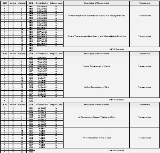
132 119

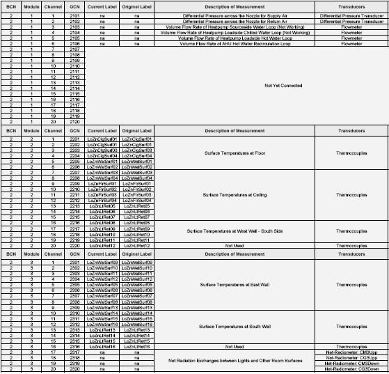
133 120

134 121

135 Appendix G: Computer Control Board Channels Table G-1 DAC channel diagram (Chantrasrisalai 2007b) 122

136 Table G-2 DAS channel layout (Chantrasrisalai 2007b) Note the safety board channels are in identical order as channels

137 Appendix H: HVAC System Diagrams Figure H-1 System diagram for the NE fan coil unit loop (Chantrasrisalai 2007b) 124

138 Figure H-2 System diagram for the SW fan coil unit loop (Chantrasrisalai 2007b) 125

139 Figure H-3 System diagram for the air handler unit loop (Chantrasrisalai 2007b) 126

140 Figure H-4 System diagram for the heat pump loops (Chantrasrisalai 2007b) 127