In the Name of God. Lectures 15&16: Radial Basis Function Networks

Transcription

1 1 In the Name of God Lectures 15&16: Radial Basis Function Networks

2 Some Historical Notes Learning is equivalent to finding a surface in a multidimensional space that provides a best fit to the training data. Cover (1965): A pattern-classification problem cast in a high-dimensional space is more likely to be linearly separable than in a low-dimensional space. Powell (1985): Radial-basis functions were introduced in the solution of the real multivariate interpolation problem. Broomhead and Lowe (1988) were the first to exploit the use of radial-basis functions in the design of neural networks. Mhaskar, Niyogi and Girosi (1996): The dimension of the hidden space is directly related to the capacity of the network to approximate a smooth input-output mapping (the higher h the dimension i of the hidden space, the more accurate the approximation will be).

3 Radial-Basis Function Networks In its most basic form Radial-Basis Function (RBF) network involves three layers with entirely different roles. The input layer is made up of source nodes that connect the network to its environment. The second layer, the only hidden layer, applies a nonlinear transformation from the input space to the hidden space. The output layer is linear, supplying the response of the network to the activation pattern applied to the input layer.

4 Radial-Basis Function Networks They are Feedforward neural networks compute activations at the hidden neurons using an exponential of a [Euclidean] distance measure between the input vector and a prototype t vector that characterizes the signal function at a hidden neuron. Originally introduced into the literature for the purpose p of interpolation of data points on a finite training set

5 In MLP

6 In RBFN

7 Architecture x 1 h 1 x 2 h 2 W 1 2 W 2 x 3 h 3 W 3 f(x) W m x n h m Input layer Hidden layer Output layer

8 Three layers Input layer Source nodes that connect to the network of its environment Hidden layer Hidden units provide a set of basis functions High dimensionality Output layer Linear combination of hidden functions

9 Linear Models A linear model for a function f(x) takes the form: The model f(.) is expressed as a linear combination of a set of m basis functions. The freedom to choose different values for the weights, derives the flexibility of f(.), its ability to fit many different functions. Any set of functions can be used as the basis set, however, models containing only basis functions drawn from one particular class have a special interest. h(x) is mostly Gaussian function

10 Special Base Functions Classical statistics - polynomials base functions: Signal processing applications - combinations of sinusoidal waves (Fourier series): Artificial neural networks (particularly in multi-layer perceptrons) - logistic functions:

11 Example the straight line A linear model of the form: f(x) = ax + b Which has two basis functions: h 1 (x) = 1, h 2 (x) = x Its weights are: w 1 = b, w 2 = a

12 Radial Functions Characteristic feature - their response decreases (or increases) monotonically with distance from a central point. The center, the distance scale, and the precise shape of the radial function are parameters of the model, all fixed if it is linear. Typical radial functions are: The Gaussian RBF (monotonically decreases with distance from the center). A multiquadric RBF (monotonically increases with distance from the center).

13 Radial functions Gaussian RBF: c: center, r: radius 2 ( x c) ) exp 2 h( x) r Multiquadric RBF h( x) r 2 ( x r c) 2 monotonically decreases with distance from center monotonically increases with distance from center

14 Radial Functions Gaussian RBF multiqradric i RBF

15 Cover s Theorem A complex pattern-classification problem cast in high-dimensional space nonlinearly is more likely to be linearly separable than in a low dimensional space (Cover, 1965)

16 Introduction to Cover s Theorem Let X denote a set of N patterns (points) x1, 1 x2, 2 x 3,, x N Each point is assigned to one of two classes: X + and X - This dichotomy is separable if there exists a surface that t separates these two classes of points.

17 Introduction to Cover s Theorem For each pattern x X define the vector: ( x) ( x), ( x),..., ( x) T 1 2 The vector (x) maps points in a p-dimensional input space into corresponding points in a new space of dimension m. Each i ( x) is a hidden function, i.e., a hidden unit m

18 Introduction to Cover s Theorem A dichotomy {X +,X - } is said to be φ-separable if there exist an m-dimensional vector w such that we may write (Cover, 1965): w T φ(x) 0, x X + w T φ(x) < 0, x X - The hyperplane defined by w T φ(x) = 0, is the separating surface between the two classes. Given a set of patterns X in an input space of arbitrary dimension p, we can usually find a nonlinear mapping φ(x) of high enough dimension m such that we have linear separability in the φ space.

19 Examples of φ-separable Dichotomies Linearly Separable Spherically Separable Quadrically Separable

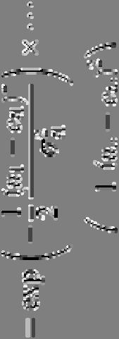
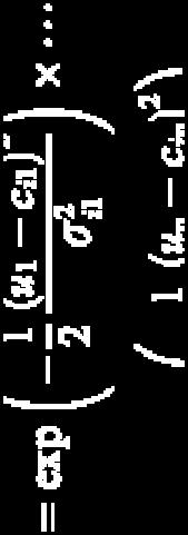
20 Back to the XOR Problem Recall that in the XOR problem, there are four patterns (points), namely, (0,0),(0,1),(1,0),(1,1), (00)(01)(10)(11) in a two dimensional input space. We would like to construct a pattern classifier that produces the output 0 for the input patterns (0,0),(1,1) and the output 1 for the input patterns (0,1),(1,0). We will define a pair of Gaussian hidden functions as follows: x t ( x) e, t x t 2 2 ( x ) e, t 2 2

21 Back to the XOR Problem Using the later pair of Gaussian hidden functions, the input patterns are mapped onto the φ 1 - φ 2 plane, and now the input points can be linearly separable as required. φ 2 φ 2 (0,0) (0,1) (1,0) (1,1) φ 1

22 Interpolation Problem Assume a domain X and a range Y taken to be metric space, and that is related by a fixed but unknown mapping f. The problem of reconstructing the mapping f is said to be well-posed if three conditions are satisfied: Existence: For every input vector x H, there does exist an output y=f(x), where y H. Uniqueness: For any pair of input vectors x,t H, we have f(x)=f(t) f(t) if, and only if x=t. Continuity: (=stability) for any >0 there exists = ( ) such that the condition x (x,t)< implies that y (f(x),f(t))<, f(t))< where (.,.) ) is the symbol for distance between the two arguments in their respective spaces.

23 Interpolation Problem Given T = {X d k } X n k, k} k, dk Solving the interpolation problem means finding the map f(x k ) = d k, k = 1,,Q (target points are scalars for simplicity of exposition) RBFN assumes a set of exactly Q non-linear basis functions φ( X - X i ) Map is generated using a superposition of these N F( x) w ( x x ) i 1 i i

24 Application of Interpolation in Signal Processing Converting digital signals to continuous signal Up-sampling

25 Uniqueness of Interpolation Problem Nearest-neighbor interpolation Linear interpolation

26 Regularized Interpolation Has Unique Answer

27 Exact Interpolation Equation Interpolation conditions Matrix definitions Yields a compact matrix equation

28 Michelli Functions Gaussian functions Multiquadrics Inverse multiquadrics

29 Solving the Interpolation Problem Choosing correctly ensures invertibility: W = -1 D Solution is a set of weights such that the interpolating surface generated passes through exactly every data point Common form of is the localized Gaussian basis function with center and spread

30 Radial Basis Function Network x 1 1 x 2 2 x n Q

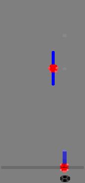
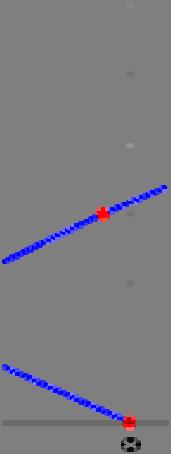
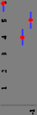
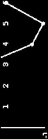
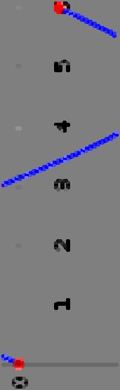
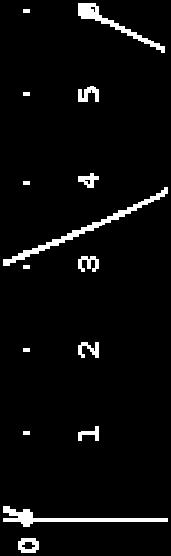
31 Interpolation Example Assume a noisy data scatter of Q = 10 data points Generator: 2sin(x) +x In the graphs that follow: data scatter (indicated by small triangles) is shown along the generating function (the fine line) interpolation shown by the thick line = 1 =

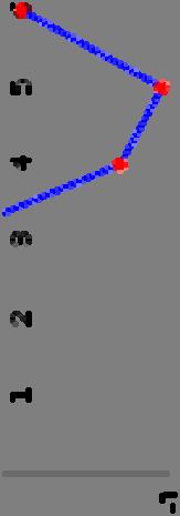
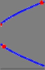
32 Derivative Square Function = 1 = 0.3

33 Notes Making the spread factor smaller makes the function increasingly non-smooth being able to achieve a 100 per cent mapping accuracy on the ten data points rather than smoothness of the interpolation Quantify the oscillatory behavior of the interpolants by considering their derivatives Taking the derivative of the function Square it (to make it positive everywhere) Measure the areas under the curves Provides a nice measure of the non-smoothness the greater the area, the more non-smooth the function!

34 Problems Oscillatory behavior is highly undesirable for proper generalization Better generalization is achievable with smoother functions which are fitted to noisy data Number of basis functions in the expansion is equal to the number of data points! Not possible to have for real-world datasets, which can be extremely large Computational and storage requirements for them can explode very quickly

35 The RBFN Solution Choose the number of basis functions to be some number q < Q No longer restrict the centers of the basis functions to be fixed to the data point values. Now made trainable parameters of the model Spreads of each of the basis functions is permitted to be different and trainable. Learning can be done either by supervised or unsupervised techniques A bias is included in the final linear superposition Assume centers and spreads of the basis functions are optimized and fixed Proceed to determine the hidden output neuron weights using the procedure adopted in the interpolation case

36 Solving the Problem in a Least Squares Sense To formalize this, consider interpolating a set of data points with a number q < Q Then, Introduce the notion of error since the interpolation is not exact Input Centre

37 Compute the Optimal Weights Differentiating w.r.t. w i and setting it equal to zero Then, This yields Equation solved using singular value decomposition where Pseudo-inverse (is not square: q Q)

38 More generalization Straightforward to include a bias term w 0 into the approximation equation Basis function is generally chosen to be the Gaussian RBFs can be generalized to include arbitrary covariance matrices K i Universal approximator RBFNs have the best approximation property The set of approximating functions that RBFNs are capable of generating, there is one function that has the minimum approximation error for any given function which has to be approximated

39 RBFN Classifier to Solve the XOR Problem Will serve to show how a bias term is included at the output linear neuron RBFN classifier is assumed to have two basis functions centered at data points 1 and 4 The basis functions

40 RBFN Classifier to Solve the XOR Problem +1 x 1 1 w 1 w 2 f x 2 2 Basis functions centered at data points 1 and 4 We have the D, W, vectors and matrices as shown alongside Pseudo inverse and weight vector

41 Ill-Posed and Well-Posed Problems Ill-posed problems originally identified by Hadamard in the context t of partial differential equations. Problems are well-posed if their solutions satisfy three conditions: they exist they are unique they depend continuously on the data set Problems that are not well-posed are ill-posed Example differentiation is an ill-posed problem because some solutions need not depend continuously on the data inverse kinematics problem which maps external real-world movements into an internal coordinate system is also an ill- posed problem

42 Approximation Problem is Ill-Posed The solution to the problem is not unique Sufficient i data is not available to reconstruct t the mapping uniquely Data points are generally noisy The solution to the ill-posed approximation problem lies in regularization essentially requires the introduction of certain constraints that impose a restriction on the solution space Necessarily problem dependent Regularization techniques impose smoothness constraints on the approximating set of functions Some degree of smoothness is necessary for the representative function since it has to be robust against noise

43 Regularization Theory Assume training data T generated by random sampling of fthe function Regularization techniques replace the standard error minimization problem with minimization of a regularization risk functional The main idea behind regularization is to stabilize the solution by means of prior information This is done by including a function in the cost function Only a small number of candidate solutions will minimize this functional These functional terms are called the regularization terms Typically, the functional measure for the smoothness of the function

44 Tikhonov Functional Regularization risk functional comprises two terms error function smoothness functional intuitively iti appealing to consider using function derivatives to characterize smoothness The smoothness functional is expressed as P is a linear differential e operator, is a norm The regularization risk functional to be minimized is regularization parameter

45 Solving the Euler Lagrange System See complete solution in the textbook! Yields the final solution (Green's function, G(x, s), of a linear differential operator L is any solution of LG(x, s) = δ(x-s), where δ is Dirac delta function) Linear weighted sum of Q Green s functions centered at the data points X i The regularization solution uses Q Green s functions in a weighted summation The nature of the chosen Green s function depends on the kind of differential operator P chosen for the regularization term of R r

46 Solving for Weights Starting point Evaluate the equation at each data point Introduce matrix notation

47 Euclidean Norm Dependence If the differential operator P is rotationally invariant translationally invariant Then, the Green s function G(X,Y) depends only on the Euclidean norm of the difference of the vectors Then,

48 Multivariate Gaussian is a Green s Function Gaussian function defined by is a Green s function defined by the self-adjoint differential operator The final minimizer is then,

49 Desirable Properties of Regularization Networks The regularization network is a universal approximator, that can approximate any multivariate continuous function arbitrarily well, given sufficiently large number of hidden units. The approximation shows the best approximation property (best coefficients i will be found). The solution is optimal: it will minimize the cost functional ( F).

50 Generalized Radial Basis Function Network We now proceed to generalize the RBFN in two steps Reduce the Number of Basis Functions, Use Non-Data Centers Use a Weighted Norm

51 Reduce the Number of Basis Functions, Use Non-Data Centers The approximating function is Interested in minimizing the regualrized risk Simplifying the first term Using the matrix substitutions yields

52 Reduce the Number of Basis Functions, Use Non-Data Centers Simplifying the second term Use the properties of the adjoint of the differential operator and Green s function where Finally And the optimal weights W are obtained as

53 Using a Weighted Norm Replace the standard Euclidean norm by S is a norm-weighting matrix of proper dimension Substituting into the Gaussian yields where K is the covariance matrix With K = 2 I is a restricted form

54 Generalized Radial Basis Function Network Some propertiesp Fewer than Q basis functions (remember Q is the number of samples) A weighted norm to compute distances, which manifests itself as a general covariance matrix A bias weight at the output neuron Tunable weights, centers, and covariance matrices

55 Estimating the parameters Weights wi : already discussed (more next). Regularization parameter : Minimize averaged squared error. Use generalized cross-validation. RBF centers: Randomly select fixed centers. Self-organized selection. Supervised selection.

56 Estimating the Regularization parameter Minimize average squared error: For a fixed, for all Q inputs, calculate the squared error between the true function value and the estimated RBF network output using the. Find the optimal that minimizes this error. Problem: This requires knowledge of the true function values. Generalized cross-validation: Use leave-one-out cross validation. With a fixed, for all Q inputs, find the difference between the target value (from the training set) and the predicted value from the leaveone-out-trained network. This approach depends only on the training set.

57 Selection of the RBF forward selection starts with an empty subset adds one basis function at a time most reduces the sum-squared-error until some chosen criterion stops backward elimination i starts with the full subset removes one basis function at a time least increases the sum-squared-error until the chosen criterion stops decreasing

58 Number of radial basis neurons By designer Max of neurons = number of patterns Min of neurons = ( experimentally determined) More neurons More complex, but smaller tolerance

59 Learning strategies Two levels of Learning Center and spread learning (or determination) Output layer Weights Learning Make # ( parameters) as small as possible Principles of Dimensionality

60 Various learning strategies how the centers of the radial-basis functions of the network are specified. 1. Fixed centers selected at random 2. Self-organized selection of centers 3. Supervised selection of centers

61 Fixed centers selected at random Fixed RBFs of the hidden units The locations of the centers may be chosen randomly from the training dataset We can use different values of centers and widths for each radial basis function -> experimentation ti with training i data is needed d

62 Fixed centers selected at random Only output layer weight is needed to be learned Obtain the value of the output layer weight by pseudo-inverse method Main problem Requires a large training set for a satisfactory level of performance

63 Self-organized selection of centers Hybrid learning self-organized learning to estimate the centers of RBFs in hidden layer supervised learning to estimate t the linear weights of the output layer Self-organized learning of centers by means of clustering Supervised learning of output weights by LMS algorithm (pseudo-inverse method)

64 Self-organized selection of centers k-means clustering

65 Supervised selection of centers All free parameters of the network are changed by supervised learning process 1 E e, e d F ( x ) d w ( n) G( x ) 2 Ci N M 2 * j j j j j i j i j 1 i 1 Use error correction learning LMS to adjust all RBF parameters to minimize the error cost function: Linear weights (output layer): ( n) wi( n 1) wi( n) 1 w( n) Position of centers (hidden layer): i( n 1) i( n) 2 i Width of centers (hidden layer): 1 1 K ( n 1) K ( n) i i i ( n) t ( n) 3 1 i ( n) ( n)

66 Learning formula Linear weights (output layer) N ( n) E( n) ej( n) G( j i( n) C ) i wi ( n) x wi ( n 1) wi ( n) 1, i 1,2,..., M j 1 w ( n) Positions of centers (hidden layer) N ' 1 i j j i C i j i j 1 En ( ) 2 w ( n) e ( n) G ( ( n) ) K [ ( n)] i ( n) x x t i i En ( ) i( n 1) i( n) 2, i 1, 2,..., M ( n) i Spreads of centers (hidden layer) 1 i N ' i( ) j( ) ( j i( ) C ) ( ) i ji j K ( n 1) K ( n ) i i 3 Ki En ( ) w n e n G x n Q n Q ( ) [ ( )][ ( )] T ji n xj i n xj i n K ( n) E( n) 3 1 ( n)

67 Testing and Comparison Tested Adaptive Center RBF against Fixed Center RBF Made use of the cost function given below Analyze differences between two networks Cost Function 1 E 2 N 2 e j j 1 e d F*( x ) d wg( x t ) j j j j i j i C i 1 M i

68 Function Approximation "Plateau" function y = f(x1,x2) used in this example. The data are sampled in the domain - 1<x1<1, -1<x2<1. G. Bugmann, et all, "CLASSIFICATION USING NETWORKS OF NORMALIZED RADIAL BASIS FUNCTIONS", ICAPR 1998.

69 Function Approximation A) Function of a standard RBF net trained on 70 points sampled from Plateau function. Parameters: σ = 0.21, 021 Average RMS error < 0.04 after 30 epochs. 50 hidden nodes B) Function of a standard RBF net with σ = Figure produced for the purpose of indicating the positions of the 70 training i data.

70 Comparison of RBF and MLP RBF has a single hidden layer, while MLP can have many In MLP, hidden and output neurons have the same underlying function. In RBF, they are specialized into distinct functions In RBF, the output layer is linear, but in MLP, all neurons are nonlinear The hidden neurons in RBF calculate the Euclidean norm of the input vector and the center, while in MLP the inner product of the input vector and the weight vector is calculated l MLPs construct global approximations to nonlinear input output mapping. RBF uses exponentially decaying localized nonlinearities (e.g. Gaussians) to construct local approximations to nonlinear input output mappings

71 Locally linear models U = [U 1, U 2,, U p ]: inputs M: number of Locally Linear Model (LLMs) neurons w ij: denotes the LLM parameters of the i-th neuron The validity functions are chosen as normalized Gaussians Normalization is necessary for a proper interpretation of validity functions

72 Locally linear models

73 Locally Linear Model Tree (LoLiMoT) learning algorithm (Nelles 2001) 1. Start with an initial model: Construct the validity functions for the initially given input space partitioning and estimate the LLM parameters. Set M to the initial number of LLMs. If no input space partitioning is available a priori, then set M=1 and start t with a single LLM, which h in fact is a global l linear model since its validity function covers the whole input space with Φ 1 (x) = 1

74 Locally Linear Model Tree (LoLiMoT) learning algorithm (Nelles 2001) 2. Find worst LLM: Calculate a local loss function for each of the i = 1,..., M LLMs. The local loss functions can be computed by weighing the squared model errors with the degree of validity of the corresponding local model according to: Find the worst performing LLM, that is max i (I i ), and denote k as the index of this worst LLM

75 Locally Linear Model Tree (LoLiMoT) learning algorithm (Nelles 2001) 3. Check all divisions: The k-th LLM is considered for further refinement. The hyper-rectangle rectangle of this LLM is split into two halves with an axis-orthogonal split. Divisions in all dimensions are tried. For each division dim=1,,p the following steps are carried out: a. Construction of the multidimensional MFs for both hyperrectangles b. Construction of all validity functions c. Local estimation of the rule consequent parameters for both newly generated LLMs d. Calculation of the loss function for the current overall model

76 Locally Linear Model Tree (LoLiMoT) learning algorithm (Nelles 2001) Initial global linear model Split along x1 or x2 Pick split that minimizes model error (residual)

77 Reading S Haykin, Neural Networks: A Comprehensive y, p Foundation, 2007 (Chapter 6).