ABSTRACT. The distribution of bubbles in nuclear reactor coolant flow is an important

Transcription

1 ABSTRACT THOMAS, AARON MATTHEW. Estimation of the Shear-Induced Lift Force on a Single Bubble in Laminar and Turbulent Shear Flows Using Interface Tracking Approach. (Under the direction of Dr. Igor A. Bolotnov). The distribution of bubbles in nuclear reactor coolant flow is an important phenomenon to understand at a fundamental level in order to improve CFD-level prediction of two-phase flow and heat transfer. In computational multiphase fluid dynamics (CMFD) this distribution is modeled utilizing interfacial forces. Typically, those forces are modeled using limited experimental data and analytical approximations with many simplifying assumptions. In the present work, the lift force on a single bubble in laminar and turbulent shear flow regimes was quantified using direct numerical simulations (DNS). A proportionalintegral-derivative (PID)-based controller was developed and implemented into the finiteelement based, interface-tracking method, multiphase flow solver (PHASTA). The PIDbased controller was used to apply control forces to the bubble, which at steady state (or quasi-steady state) equalized the net force in the stream-wise direction and in the velocity gradient (lateral) direction. The control forces were then extracted in order to quantify the resulting lift and drag coefficients, dependent on such parameters as shear rate and relative velocity. A number of uniform shear ( s -1 ) laminar flows were simulated between two plates to extract lift and drag data for assessment against what is in literature and use as a basis for comparison against high shear turbulent flows of approximately s -1 and s -1.

2 Copyright 2014 Aaron Matthew Thomas All Rights Reserved

3 Estimation of the Shear-Induced Lift Force on a Single Bubble in Laminar and Turbulent Shear Flows Using Interface Tracking Approach by Aaron Matthew Thomas A thesis submitted to the Graduate Faculty of North Carolina State University in partial fulfillment of the requirements for the degree of Master of Science Nuclear Engineering Raleigh, North Carolina 2014 APPROVED BY: Dr. Igor A. Bolotnov Committee Chair Dr. Joseph M. Doster Dr. Nam Dinh Dr. Alexei V. Saveliev

4 DEDICATION The first principle is that you must not fool yourself and you are the easiest person to fool. Richard P. Feynman ii

5 BIOGRAPHY The author graduated from North Carolina State University (NCSU) with a Bachelor of Science degree in Nuclear Engineering in May As an undergraduate student at NCSU, he was invited by the Consortium for Advanced Simulation of Light Water Reactors (CASL) to embark on a research project, which later evolved into his thesis work. During his undergraduate studies, he held two summer internships; one was at legacy Progress Energy s Brunswick Nuclear Plant in Southport, North Carolina, and the other was for the U.S. Nuclear Regulatory Commission (NRC) in Rockville, Maryland. He also completed a summer study abroad in Vienna, Austria, which helped him obtain an undergraduate minor in the German language. The undergraduate research had helped fuel his interest in getting a Master of Science degree in Nuclear Engineering. With that, he pursued an M.S. degree in the accelerated bachelor-master program in the Nuclear Engineering department at NCSU, allowing him to complete the M.S. degree within a year. During his graduate year at NCSU, he passed the Fundamentals of Engineering exam and became professionally designated as an Engineer in Training (EIT) by the National Council of Examiners for Engineering and Surveying. The author accepted a full-time position with the U.S. NRC starting after the completion of his Master degree. He was accepted into the Nuclear Safety Professional Development Program (NSPDP) in the Office of New Reactors (NRO), Division of Safety Systems and Risk Assessment (DSRA), Reactor Systems, Nuclear Performance, and Code Review Branch (SRSB). In his free time, the author enjoys driving his Mini Cooper down back-country, twisty, mountain roads. iii

6 ACKNOWLEDGMENTS I would like to give my ultimate thanks to God, as he has given me absolutely everything in this world that has allowed me to get where I am today. I am so incredibly thankful for my family; my father who has meticulously instilled in me the fundamental traits of an engineer and has taught me how to live humbly, my mother who has shown me how to be thankful for every single blessing in my life and has shown me persistent support in everything I do, and my older brother, whom I ve looked up to since I was born. My family has shown me abundant, unconditional love, which has undoubtedly helped me get to where I am today. I express my deepest gratitude to Dr. Bolotnov, as his undiminished intelligence in the field of two-phase bubbly flow has created my knowledge foundation for which I will always grow upon. I also want to express exceptional recognition to Jun Fang, whose pure brilliance has encourage critical thinking and innovative discussion which has genuinely helped me understand fundamental two-phase flow phenomenon. I extended my utmost appreciation to Ms. Marshall, who has been incredible at giving me academic and professional advice that has certainly made some hard decisions for me easy. I would like to acknowledge the Consortium for Advanced Simulation of Light Water Reactors as being a key element of my success in this research, as this was what sparked my interest in reactor thermal hydraulics, and more importantly, bubbles. The U.S. Nuclear Regulatory Commission had funded a fellowship that I was awarded by my department; my deepest appreciation goes out to them. iv

7 I d like to express my sincere appreciation to my committee members, Dr. Doster, Dr. Dinh, and Dr. Saveliev for serving on my committee. Dr. Saveliev was my undergraduate fluid mechanics professor and graduate heat transfer professor in the mechanical engineering department, and ultimately gave me my first introduction into fluid mechanics. I attended Dr. Dinh s graduate level nuclear reactor severe accident safety analysis course. Dr. Dinh s wisdom and knowledge in the realm of severe accidents is immense and his teachings will certainly help guide me through my future career. Dr. Doster was my nuclear reactor thermal hydraulics professor. His intelligence in this field of study is immeasurable and I am very fortunate to have had him as a professor. I d also like to extend my genuine gratitude to the whole Nuclear Engineering Department at NCSU. Many of the faculty, staff, and graduate students have given me invaluable help and assistance throughout my academic career. I want to thank all of my friends for being there for me since the beginning of time. I really appreciate an unforgettable laugh and camaraderie, and my friends have certainly given this to me. Murica! v

8 TABLE OF CONTENTS LIST OF TABLES... ix LIST OF FIGURES... xii 1. INTRODUCTION Literature Review PROBLEM FORMULATION Numerical Method Overview Governing equations The level set method Bubble Control Problem Bubble control algorithm PID Control Bubble control application Case Description Overview Low shear laminar cases Transition laminar cases High shear laminar and turbulent cases High shear turbulent cases setup vi

9 2.3.4 Domain Size Study PWR Fluid Properties Cases RESULTS AND DISCUSSION General Overview and Discussion Mesh Study Validation Low Shear Laminar Cases Transition Laminar Cases High Shear Cases High shear laminar cases High shear turbulent cases High turbulent shear 236 s -1 discussion High turbulent shear 470 s -1 discussion Domain Size Study Results PWR Fluid Properties Cases Computational Costs Estimate CONCLUSIONS Future Work vii

10 REFERENCES APPENDICES Appendix A Appendix B Appendix C Appendix D Appendix E viii

11 LIST OF TABLES Table 1: Mass and volume of pure gas and interface region of a bubble Table 2: Fluid properties Table 3: Low shear laminar case space Table 4: Transition from low to high shear flow case space Table 5: Transition shear case control parameters Table 6: High shear laminar and turbulent case space Table 7: High shear laminar and turbulent case control parameters Table 8: Friction Reynolds number based on shear rate Table 9: Boundary layer mesh spacing Table 10: Boundary layer mesh spacing parameters Table 11: Shear 20 s -1 large domain case parameters Table 12: PWR fluid properties Table 13: PWR fluid properties case space Table 14: Mesh refinement study: mesh parameters Table 15: Mesh refinement study: results Table 16: Window averaged lift and drag coefficients for fine mesh case Table 17: Drag coefficients for low shear laminar cases Table 18: Lift coefficients for low shear laminar cases Table 19: Drag coefficients for transition shear laminar cases Table 20: Lift coefficients for transition shear laminar cases Table 21: Drag coefficients for high shear rates of 236 s -1 and 470 s ix

12 Table 22: Lift coefficients for high shear rates of 236 s -1 and 470 s Table 23: Estimated drag coefficients for high shear turbulent cases Table 24: Estimated lift coefficients for high shear turbulent cases Table 25: Lift and drag coefficients for high shear turbulent 236 s -1 case implementing minimum v rel limit Table 26: Lift and drag coefficients for high shear turbulent 236 s -1 case manually choosing temporal averaging interval Table 27: Drag and lift coefficients estimated for normal and large size domain with shear rate of 20 s Table 28: Estimated drag coefficients for shear rates 20 s -1 and 100 s -1 with PWR saturated fluid properties Table 29: Estimated lift coefficients for shear rates 20 s -1 and 100 s -1 with PWR saturated fluid properties Table 30: CPU-hour estimate for shear 50 s -1 (laminar), 100 s -1 (laminar), 236 s -1 (laminar and turbulent) Table 31: Total CPU-hour for a single week on Insight HPC machine Table 32: VANTAGE+ fuel assembly design for McGuire NPP (Duke Energy, 2003) Table 33: Typical fluid properties of a coolant channel Table 34: Approximate relative velocities of small spherical bubbles in sub-channel Table 35: Approximate shear rate values close to the wall of typical PWR fuel rod Table 36: y + values computed adjacent to interface for shear 110 s -1 and 236 s x

13 Table 37: y + values computed adjacent to the interface for the mesh study cases of 20 elements and 24 elements across the width of the bubble xi

14 LIST OF FIGURES Figure 1: Multi-bubble simulation of turbulent flow (Bolotnov et al., 2011) Figure 2: Low shear laminar flow case Figure 3: High shear laminar flow case Figure 4: High shear turbulent flow case production Figure 5: Boundary layer mesh for turbulent shear cases Figure 6: Turbulent kinetic energy (left) and mean velocity profile (right) for turbulent shear case of Re τ = 130 (window 1 defined by solid line, window 2 defined by dotted line, window 3 defined by dashed line) Figure 7: Turbulent kinetic energy (left) and mean velocity profile (right) for turbulent shear case of Re τ = 191 (window 1 defined by solid line, window 2 defined by dotted line, window 3 defined by dashed line) Figure 8: Large domain setup for shear rate of 20 s Figure 9: Diagram of how control force can abruptly change magnitude and sign in a high shear, low relative velocity flow Figure 10: Grid resolution study, 16, 20, and 24 elements across the bubble (left to right) Figure 11: Fine mesh case control force vs. time Figure 12: Estimated drag coefficients from PHASTA plotted against bubble Reynolds number. The correlation, shown as dashed line, comes from (Tomiyama et al., 1998) Figure 13: Steady state bubble shape for shear 1.0 s -1 (left) and for shear 10.0 s -1 (right) Figure 14: Whole domain control for shear = 1.0 s -1 and v rel = m/s Figure 15: Flow around bubble for shear 50 s xii

15 Figure 16: Flow around bubble for shear 110 s Figure 17: Velocity profile around bubble for high shear of 110 s -1 at different times Figure 18: Drag coefficient as a function of shear rate Figure 19: Lift coefficient as a function of shear rate Figure 20: Flow around bubble in a high shear of s Figure 21: Flow around bubble in a high shear of s Figure 22: Vortical structure interaction with bubble for shear rate of 470 s Figure 23: Relative velocity as a function of time for the high shear turbulent 236 s -1 case.. 72 Figure 24: Bubble position and velocity plots for high turbulent shear 236 s Figure 25: Control force as a function of time for high turbulent shear of 236 s Figure 26: Time evolution of a bubble in a high turbulent shear of 236 s Figure 27: Relative velocity as a function of time for high turbulent shear of 470 s Figure 28: Time evolution of a bubble in a high turbulent shear of 470 s Figure 29: Bubble position and velocity plots for the high turbulent shear 470 s -1 case Figure 30: Bubble control force as a function of time for the high turbulent shear 470 s -1 case Figure 31: Steady state flow for large domain case, shear 20 s Figure 32: Steady state flow for the shear rate of 20 s -1 using PWR saturated fluid properties Figure 33: Control force as a function of time for the shear 20 s -1 case with PWR saturated fluid properties xiii

16 Figure 34: Control force as a function of time for the shear 100 s -1 case with PWR saturated fluid properties Figure 35: Flow around bubble for the shear rate of 100 s -1 using PWR saturated fluid properties Figure 36: Mean sub-channel velocity profile in typical PWR coolant channel Figure 37: Mean shear rate in sub-channel of typical PWR Figure 38: Control force vs. time: 1.0 s -1 shear, m/s relative velocity, 5 mm bubble. 115 Figure 39: Control force vs. time: 2.0 s -1 shear, 0.05 m/s relative velocity, 5 mm bubble Figure 40: Control force vs. time: 5.0 s -1 shear, 0.05 m/s relative velocity, 5 mm bubble Figure 41: Control force vs. time: 10.0 s -1 shear, 0.05 m/s relative velocity, 5 mm bubble. 116 Figure 42: Control force vs. time: 10.0 s -1 shear, m/s relative velocity, 1 mm bubble Figure 43: Control force vs. time: 20.0 s -1 shear, m/s relative velocity, 1 mm bubble Figure 44: Control force vs. time: 30.0 s -1 shear, m/s relative velocity, 1 mm bubble Figure 45: Control force vs. time: 40.0 s -1 shear, m/s relative velocity, 1 mm bubble Figure 46: Control force vs. time: 50.0 s -1 shear, m/s relative velocity, 1 mm bubble Figure 47: Control force vs. time: 75.0 s -1 shear, m/s relative velocity, 1 mm bubble xiv

17 Figure 48: Control force vs. time: s -1 shear, m/s relative velocity, 1 mm bubble Figure 49: Control force vs. time: s -1 shear, m/s relative velocity, 1 mm bubble Figure 50: Control force vs. time: s -1 laminar shear, m/s relative velocity, 1 mm bubble Figure 51: Control force vs. time: s -1 laminar shear, m/s relative velocity, 1 mm bubble Figure 52: Control force vs. time: s -1 turbulent shear, m/s relative velocity, 1 mm bubble Figure 53: Control force vs. time: s -1 turbulent shear, m/s relative velocity, 1 mm bubble Figure 54: Control force vs. time: 20.0 s -1 shear, large domain, m/s relative velocity, 1 mm bubble Figure 55: Control force vs. time: 20.0 s -1 shear, PWR fluid properties, m/s relative velocity, 1 mm bubble Figure 56: Control force vs. time: s -1 shear, PWR fluid properties, m/s relative velocity, 1 mm bubble xv

18 1. INTRODUCTION The migration of bubbles in nuclear reactor coolant channels is an important phenomenon to understand at a fundamental level in order to best predict two-phase flow and heat transfer characteristics. As the nuclear industry advances to generation III+ and generation IV reactor technology, state-of-the-art two-phase flow correlations are highly sought after to complement the existing models. Development and improvement of the current thermal-hydraulic multiphase flow models is an important area of research (Lahey, 2005). With the rapid advances in high performance computing (HPC), direct numerical simulations (DNS) coupled with interface tracking methods (ITM) emerge as a valuable tool for analyzing complex, two-phase flow phenomenon that would otherwise be more difficult to study and analyze in an experimental setup (Bolotnov, Jansen, Drew, Oberai, & Lahey, 2011; Bolotnov, 2013); Figure 1 shows an example where the effect of bubbles on turbulent flow using the aforementioned computational tools were quantified (Bolotnov et al., 2011). Computational multiphase fluid dynamics (CMFD) codes utilize closure laws for the interfacial forces that govern the bubble distribution in the domain. The interfacial closure laws rely on experimental data and simplified analytical solutions (Drew & Passman, 1998). DNS can complement the experimental database to obtain improved closure laws for interfacial forces. This would lead to more accurate predictions of heat transfer and flow characteristics leading up to and during reactor transients. 1

19 Figure 1: Multi-bubble simulation of turbulent flow (Bolotnov et al., 2011). Bubbles lateral distribution in nuclear reactor coolant channels is dictated by the shear-induced lift force (Auton, 1987; Drew & Lahey, 1987; Zun, 1980). The lateral trajectory and distribution of bubble clusters in a channel ultimately affect turbulence production (Mazzitelli & Lohse, 2003; Mazzitelli, Lohse, & Toschi, 2003); furthermore, turbulence greatly enhances the heat flux from the fuel rods to coolant. With the use of massively parallel DNS codes, multi-bubble cases can be run to extract more knowledge about shear-induced lateral movement of bubble clusters compared to the amount of knowledge extracted from simulations using mean velocity profiles and void fraction. Developing extensive lift force correlations based on relative velocity, local liquid shear rate, lateral position, and bubble deformability, to name a few, will help better predict the lateral distribution of bubbles in CMFD (Lahey, 2005) codes allowing for accurate heat transfer and flow predictions in transient scenarios. 2

20 The main goal of the present study is to employ DNS coupled with ITM and utilize HPC in order to resolve the lift force on a single bubble in laminar, and turbulent, high shear flows, for which current data and knowledge is limited. This will allow for future studies to capitalize on these computational developments and improvements allowing for simulation of full-fledged reactor coolant environments in which the shear-induced lift phenomenon can be correlated for highly complex geometries and validated against the current database. 1.1 Literature Review The ongoing development of a comprehensive shear-induced lift force model has been characterized into three main categories: (1) analytical; (2) numerical; (3) experimental (Hibiki & Ishii, 2007). In this extensive study the current status and improvements in lift force model development for single particle systems were summarized. Pioneering work has made several assumptions in order to derive an analytical form of the lift force which is valid for a limited number of low shear flows (Saffman, 1965; 1968). This and other analytical lift approximations are too basic for use in complex flows, where bubble shape (Ervin & Tryggvason, 1997; Tomiyama, 2004), location with respect to a wall (Cherukat & McLaughlin, 1994), turbulence (Pascal & Oesterlé, 2000; Sridhar & Katz, 1995), and many other factors all influence the shear-induced lift phenomenon. Numerical work has provided a lift coefficient expression for shear rates between 0 and 1; where the shear rate is defined as the ratio between the velocity difference across the bubble and the relative velocity (Legendre & Magnaudet, 1998). The first demonstrations of the existence of the lift force were completed experimentally (Segré & Silberberg, 1962a; 1962b), and pioneering experiments on the lateral migration using bubble trajectories proved to be fundamental 3

21 (Kariyasaki, 1987). This early experimental work has recently been quantified (Liu, 1993), and empirically correlated (Tomiyama, Tamai, Zun, & Hosokawa, 2002). These empirical models correlate the lift coefficient for small bubbles as a function of the bubble Reynolds number. In the realm of recent experimentation, it was suggested that there still exists an insufficiency in the amount of knowledge on the lateral movement of bubbles in shear flows due to the lack of experimental results (Tomiyama et al., 2002). One of the most recognized characteristics of the lift force in an up-flow condition is that small bubbles tend to migrate toward a channel wall, whereas larger bubbles tend to migrate toward a channel center (Zun, 1988); (Liu, 1993); (Hibiki & Ishii, 1999); (Hibiki, Ishii, & Xiao, 2001; Hibiki, Situ, Mi, & Ishii, 2003), or more generally, the surface tension greatly affects the direction of the lift force (Ervin & Tryggvason, 1997). Low surface tension can allow for bubble deformation and result in a sign flip in the lift force which was shown experimentally (Ervin & Tryggvason, 1997; Tomiyama et al., 2002; Tomiyama, 2004), and was in agreement with numerical work (Takagi & Matsumoto, 1995). A numerical study suggested that the interaction between the bubble s wake, shear flow regime, and internal gas flow of the bubble strongly affect the lateral migration (Tomiyama, Zun, Sou, & Sakaguchi, 1993); it was also found that the Eötvös and Morton numbers play an essential role in the direction and magnitude of the lateral migration. The direction of lateral migration was presumed to be governed by a complex interaction between the bubble s wake and the shear velocity field around the bubble (Serizawa & Kataoka, 1994). The validity of the presumption, which was based off a survey of experimental data, was partly confirmed (Tomiyama et al., 1993; Tomiyama, Sou, Zun, 4

22 Kanami, & Sakaguchi, 1995) by interface tracking simulations of single bubbles in Poiseuille flow. The complex interaction between the bubble s wake and the shear velocity profile seems to be a highly understudied phenomenon as there is not much available data to reference. One of the most widely used lift force correlations (Tomiyama et al., 2002), which was used in the present work for a basis of comparison, was experimentally developed for high viscosity systems. The study used a mixture of glycerol and water to correlate the lift force by tracking single bubble trajectories. The transverse force due to a bubble s slanted wake as separate from the shear induced lift force (but same function form) was also correlated; the sum of the shear induced lift force and the slanted wake induced lift force equals the net transverse lift force (Tomiyama et al., 2002). However, this experimentally developed correlation may not be applicable to low viscosity systems, such as air and water. Using full, 3-dimensional, volume of fluid (VOF), numerical simulations a single bubble in a low viscosity shear flow was recently investigated (Zhongchun, Xiaoming, Shengyao, & Jiyang, 2014). Comparison between high and low viscosity systems, a large bubble in a low viscosity shear flow followed an oscillating path towards the moving wall and experienced deformation. As the viscosity of the liquid was decreased, the oscillation amplitude increased. A small bubble in low viscosity shear flow migrated to the stationary wall with larger velocity than that in the high viscosity fluid, and no deformation occurred. It was reported that the asymmetrical wake of the bubble triggered the oscillation behavior (Magnaudet & Mougin, 2007; Zhongchun et al., 2014). For a small, spherical air bubble in 5

23 water, the lift coefficient was estimated to be much larger than that for a similar bubble in a higher viscosity fluid. The lift force work has been extended to turbulent flows by theoretical and computational studies (Sene, Hunt, & Thomas, 1994), which show that bubbles collecting on the downflow side of a vortex is strongly dependent on the lift force. Experimental work (Sridhar & Katz, 1999) found that bubbles become entrained in vortices and accumulate on the vortex s downward flow side also. DNS studies (Mazzitelli & Lohse, 2003; Mazzitelli et al., 2003) confirm this experimental work in which the lift force enhances bubble accumulation in this particular area of vortices, which results in a slower bubble rise velocity. It was reported (L. Wang & Maxey, 1993) that accumulations of bubbles in isotropic turbulence occur in regions of high vorticity and low pressure, where the Kolmogorov scale is more important than energy-containing scales used for dispersion quantification. Confirmation (Giusti, Lucci, & Soldati, 2005) with DNS showed that gravity and the lift force are the dominating factors in microbubble dispersion in the wall region of a channel; more specifically, in downward flow, the bubble rise velocity produces a lift force which pushes the bubble away from the wall and in upward flow, the lift force pushes the bubble towards the wall, which was also noted earlier (Hibiki, Goda, Kim, Ishii, & Uhle, 2004; S. K. Wang, Lee, Jones, & Lahey, 1987). 6

24 2. PROBLEM FORMULATION 2.1 Numerical Method Overview PHASTA is a Parallel, Hierarchic, higher-order, Adaptive, Stabilized (finite element method-based [FEM]) Transient Analysis multiphase flow solver for both incompressible and compressible flows. The flow solver has been proven to be an effective tool for a multitude of different types of simulations including, Reynolds-averaged Navier-Stokes (RANS), Large-eddy Simulation (LES), Detached-eddy Simulation (DES), and DNS (Jansen, 1999; Whiting & Jansen, 2001). Benchmarks (Jansen, 1993) have validated the PHASTA code for simulation of turbulent flows. PHASTA and its advanced features, such as anisotropic adaptive algorithms (Sahni, Mueller, Jansen, Shephard, & Taylor, 2006) and the LES/DES models (Tejada-Martinez & Jansen, 2005) have been coupled with an interface tracking method (Nagrath, Jansen, Lahey, & Akhatov, 2006) known as the level set method (Sethian, 1999; Sussman, Fatemi, Smereka, & Osher, 1998; Sussman et al., 1999; Sussman & Fatemi, 1999). PHASTA is capable of using anisotropically adapted unstructured grids or regular grids and being highly scalable for performing on massively parallel computers (Bolotnov et al., 2011; Bolotnov, 2013; Zhou et al., 2010) Governing equations The spatial and temporal discretizations for the Incompressible Navier-Stokes (INS) equations used in the FEM code have been described in (Nagrath, 2004; Whiting, 1999). The strong form of the INS equations is given by: Continuity: u ii,j = 0 ( 1 ) 7

25 Momentum: ρρu ii,t + ρρu j u ii,j = pp,ii + τ iij,j + f ii ( 2 ) where ρρ is density, u i is the i th component of velocity, p is the static pressure, τ ij is the viscous stress tensor, and f i is the body force along the i th coordinate. The viscous stress tensor for an incompressible flow of a Newtonian fluid is related to the fluid's dynamic viscosity, μ, and the strain rate tensor, S ij, as: τ iij = 2μS iij = μ(u ii,j + u j,ii ) ( 3 ) Using the Continuum Surface Tension (CST) model (Brackbill, Kothe, & Zemach, 1992), the surface tension force is computed as a local interfacial force density, which is included in f i. For the explicit treatment of surface tension to be stable, the time step must be chosen small enough in order to resolve the propagation of capillary waves. The time step becomes on the order of Δt s (Δx) 3/2 (Brackbill et al., 1992). t s < ρρ ( xx)3 2πσ 1 2 ( 4 ) ρρ is the arithmetic average of the phasic densities, Δx is the element width, and σ is the surface tension. 8

26 2.1.2 The level set method As mentioned earlier, PHASTA employs the level set method (Sethian, 1999; Sussman et al., 1998; 1999; Sussman & Fatemi, 1999) in order to track phasic interfaces. The actual gas-liquid interface of a bubble is modeled as the zero-level set of a smooth function, φ, where φ is called the first scalar and is represented as the signed distance from the zerolevel set. Naturally, where φ = 0, the level set defines the interface. The scalar, φ, is advected with the fluid according to the advection equation: Dφ Dt = φ + u φ = 0 ( 5 ) t where u is the flow velocity vector. The liquid phase, phase-1, is indicated by a positive level set, φ > 0, and the gas phase, i.e. phase-2, is indicated by a negative level set, φ < 0. It can be easily imagined that poor computational results manifest when evaluating the jump in physical properties across the interface using a step change. To remedy this, the properties near the interface are defined according to a smoothed Heaviside kernel function, H ε, (Sussman et al., 1999): H ε (φ) = 0, φ < ε φ ε + 1 π sin πφ, φ < ε ε 1, φ > ε ( 6 ) where ε is the interface half-thickness. The fluid properties can then be evaluated as: 9

27 ρρ(φ) = ρρ 1 H ε (φ) + ρρ 2 1 H ε (φ) ( 7 ) μ(φ) = μ 1 H ε (φ) + μ 2 1 H ε (φ) ( 8 ) It turns out that the solution is relatively accurate in the close vicinity of the interface. However, the level set distance field, φ, may not be as correct elsewhere in the domain, for example, at locations experiencing varying fluid velocities where the level set contours become distorted, such as in fully resolved turbulent flow simulations. A re-distancing operation was introduced for correction of the distorted distance field (Sussman & Fatemi, 1999): dd = S(φ)[1 dd ] ( 9 ) τ where d is a scalar that represents the corrected distance field, and τ is the pseudo time over which Equation ( 9 ) is solved to steady state. Equation ( 9 ) can be expressed as a transport equation: dd + w dd = S(φ) ( 10 ) τ The second scalar, d, is initially assigned the level set field, φ, and is convected with a pseudo velocity, w, where: 10

28 w = S(φ) dd dd ( 11 ) and S(φ) is defined as: 1, φ < ε d S(φ) = φ + 1 sin πφ, φ < ε ε d π ε d ( 12 ) d 1, φ > ε d where ε d is the distance field interface half-thickness (which may be different from ε used in Equation ( 6 ). The zero-level set, φ = 0, does not move since its convecting velocity is zero. Solving Equation ( 10 ) to steady state restores the distance field so that d = ±1 but does not change the location of the interface. The steady state solution of the second scalar, d, is then used to update the first scalar, φ. An additional constraint on the re-distancing step was applied to help ensure the interface did not move (Sussman et al., 1999; Sussman & Fatemi, 1999). The constraint functioned as a preservative for the original phasic mass during the re-distancing procedure. Imposing this has been found to improve convergence (Bolotnov et al., 2011). 2.2 Bubble Control Problem A bubble in a shear flow experiences a lift force which acts in the direction of the velocity gradient due to four fundamental factors: (i) the relative velocity between the bubble and surrounding fluid, (ii) the shear rate of the surrounding fluid, (iii) the bubble rotational speed, and (iv), the bubble surface boundary condition (Hibiki & Ishii, 2007). The drag force 11

29 which acts in the direction of liquid velocity is due to the relative velocity between the bubble and surrounding fluid. Therefore, a bubble being simulated in a shear flow will migrate laterally according to the direction and magnitude of the lift force with the following functional form (Drew & Lahey, 1987; Zun, 1980): FF L = CC L ρρ l V b vv r ccurl(vv l ) ( 13 ) where: ccurl(vv l ) = ddvv l ( 14 ) ddy vv r = vv g vv l ( 15 ) and will flow in the stream-wise direction according to the balance of the drag and the buoyancy force: FF D = 1 2 CC Dρρ l vv r 2 A ( 16 ) FF B = ρρ l ρρ g V b g ( 17 ) 12

30 where CC L is the lift coefficient, ρρ l and ρρ g are the densities of the liquid and gas phase, respectively; V b is the bubble volume, vv l and vv g are the velocities of the liquid and gas phase, respectively; vv r is the relative velocity between the liquid and gas phase, CC D is the drag coefficient, A is the bubble s cross sectional area projected onto the plane normal to the direction of flow, and g is gravity. The goal of this study is to compute the lift and drag coefficient for a single bubble in turbulent and laminar shear flows. If the bubble can be externally influenced so that over the simulation time, the bubble s position remains approximately constant, then the fabricated control forces applied to the bubble to control its position would balance the natural forces due to lift, drag, and buoyancy, thus the motivation for the bubble control algorithm (Thomas & Bolotnov, 2012). At steady state (or quasi-steady state), the PID-based controller applies forces in each direction to balance the net forces caused by the lift, drag, and buoyancy; therefore, keeping the bubble stationary. A static, non-moving bubble implies that the sum of the forces in each direction is zero. A force balance on the bubble is given by: FF D = (FF B + FF xc ) = ρρ l ρρ g V b g x + FF xc = 1 2 CC Dρρ l vv r 2 A ( 18 ) where FF xc is the control force applied by the controller in the x-direction, and: FF L = FF yc = CC L ρρ l V b vv r ddvv l ( 19 ) ddy 13

31 where FF yc is the control force applied by the controller in the y-direction. It is assumed here that gravity acts in the x-direction, thus the buoyancy force acts in the x-direction, and that drag acts in the x-direction (where the drag force in the y-direction is negligible). Since the flow moves in the x-direction, v r is a three component vector where the y and z components are negligible. Analysis of Equations ( 18 ) and ( 19 ) allowed for two different control force implementation ideas to be developed. (I): Applying the control force to the whole domain as pseudo-gravity. This alters the buoyancy forces, which in turn balances the lift and drag force at steady state; we ll denote this as the whole domain control method. (II): Applying the control force only to the inside of the bubble and setting the gravity in the domain to zero so that FF B in Equation ( 18 ) vanishes; we ll refer to this as the bubble control method Bubble control algorithm As part of this research, the PHASTA ITM code has been equipped with a proportional-integral-derivative (PID)-based controller that applies forces, which equally balance the net forces (caused by lift, drag, and buoyancy) on the bubble at steady state (Thomas & Bolotnov, 2012). The control forces can be extracted from the simulation and used to compute lift and drag coefficients based on Equation ( 18 ) and Equation ( 19 ) (Fang, Thomas, & Bolotnov, 2013) PID Control A PID controller consists of three error feedbacks; P which represents the proportional term, or the present error, I, the integral term, which represents the accumulation of past errors, and D, the derivative term, which represents the prediction of future errors. In the bubble control algorithm, the error input for the controller can be thought of as the 14

32 distance the bubble moves away from its initial location. For each simulated time step, the PID-based bubble controller assesses the bubble location and velocity and uses those variables as inputs for control loop feedback. The functional form of the PID-based bubble controller is as follows: CCFF (nn+1) ii = cc 1 CCCC (nn) ii + cc 2 CCFF (nn) ii + cc 3 ddxx (nn) ii + cc 4 ddxx 2 (nn) ii + cc5 ddxx 3 (nn) ii + cc6 vv (nn) ii + cc 7 vv 2 (nn) ii + cc 8 vv 3 (nn) ii + cc9 ddvv (nn) ii + cc 10 ddxx 2 (nn) 2 iiii ( 20 ) ii=1 where CCFF (nn) ii is the i th component of the control force at time n, CCCC (nn) ii is the historical average of the i th component of control at time n, ddxx ii (nn) is the i th component of the difference in the bubble s location at time n and time zero, vv ii (nn) is the i th component of the bubble s average velocity at time n, ddvv ii (nn) is the i th component of the difference in the bubble s average velocity at time n and time n-1, ddxx 2 (nn) ii and ddxx 3(nn) ii are the i th components of the difference in the bubble s location at time n and time zero squared, and cubed, respectively, vv 2 (nn) ii and vv 3 (nn) ii are the i th components of the bubble s average velocity at time n squared, and cubed, respectively, and c k, for k=1,..,10, are controller gains. The vector component convention used in this work is i=1 refers to the x-component, i=2 refers to the y-component, and i=3 refers to the z-component. Equation ( 20 ) can be simplified to the following form, as it was determined that many of the higher order terms were not necessary for obtaining the results presented in this paper. 15

33 CCFF (nn+1) ii = pp 1 CCCC (nn) ii + pp 2 CCFF (nn) ii + pp 3 ddxx (nn) ii + pp 4 ddxx 2 (nn) ii + pp5 vv (nn) ii ( 21 ) Analysis of Equation ( 20 ) reveals a PID-based form. The historical average, CCCC (nn) ii, is analogous to the integral input, the linear, and higher order location difference terms function as the proportional input, and the velocity and velocity difference terms resemble the derivative input Bubble control application The application and implementation of Equation ( 20 ) into the PHASTA ITM code was an extensive learning process. In order for the control forces computed by the PID-based controller to be added into the right-hand side (RHS) body force term of Equation ( 2 ), several obstacles had to be overcome. First, PHASTA was equipped with a bubble position and velocity tracking algorithm. Simply enough, at each time step the positions of every node inside the bubble were averaged to obtain the bubbles average position. The velocities, on the other hand, required a bit more complex averaging scheme in order to resolve the bubble s total average velocity. As mentioned earlier, PHASTA treats the liquid-gas interface as a finite thickness of continuously smoothed liquid-gas properties. In order to properly compute the bubble s average velocity, it was shown that the elemental velocities inside the bubble (which includes the bubble s interface with the liquid) needed to be weighted by element volumes and element densities. 16

34 u ii = N j=1 N j=1 ρρ l ρρ j V j u ii,j ρρ l ρρ j V j ( 22 ) where u ii is the i th component of the bubble s average velocity, N is the number of elements inside the pure gas part of the bubble plus the interface shell, ρρ j is density of the fluid in the j th element, V j is the volume of the j th element, and u ii,j is the i th component of velocity in the j th element inside the bubble. It can be shown that with the addition of the finite interface to the bubble, the bubble actually takes on a significant portion of mass and volume, which must be accounted for when averaging properties of the bubble and its interface. Table 1 shows the mass and volume of the pure gas region and the smoothed property interface region for a 1 mm in diameter bubble with interface thickness of 0.12 mm. It must be noted that overall bubble mass is correct when the interface thickness approaches zero, and does not change for a finite interface thickness. Table 1: Mass and volume of pure gas and interface region of a bubble Volume (mm 3 ) Mass (gm) Gas e-7 Interface e-4 The gas volume and mass are defined as, respectively: 17

35 V g = 4 3 π(r bub ε ls ) 3 ( 23 ) M g = ρρ g V g ( 24 ) The interface volume and mass are defined as, respectively: V iinnteriiace = 4 3 π(r bub + ε ls ) 3 V g ( 25 ) M iinnteriiace = ρ g+ρ l V 2 iinnteriiace ( 26 ) ε ls is the interface half-thickness, and r bub is the radius of the bubble where the zero-level set resides. Note that the density used in Equation ( 26 ) is an average of the liquid phase and the gas phase. Analysis shows that the theoretical average density in the smoothed property interface region is that of a simple arithmetic average. Secondly, the PID-based control function needed to be implemented into PHASTA. This required implementing the computation, averaging, and application routines spanning many different modules of the main program (See Appendix C). PHASTA s discretization of the momentum equations requires that the body forces are on a unit-mass basis, hence the control force needed to be implemented on a unit-mass basis as well. Averaging of the control force also had to take into account element volumes, in case of local mesh refinement in unstructured grid cases, and fluid density, in order to account for the varying properties 18

36 across the interface. Apart from all the other logistics of algorithm implementation, and data post processing, the PHASTA ITM code was equipped with the capability of PID-based bubble control. The control force application procedure also posed a challenging problem initially. As mentioned earlier, there are two methods of bubble control. The whole domain control method utilized manipulation of gravity throughout the domain to achieve buoyancy forces which balanced the lift and drag forces. For low complexity flows (low shear, low relative velocity, laminar flows) the whole domain method proved to be more robust and allowed for quick control convergence. However, as the shear rates and relative velocities increased, this method proved to be futile due to the need for large changes in gravity to balance the larger lift and drag forces. The large changes in gravity resulted in numerical divergence of the pressure Poisson equation solve at the prescribed velocity outflow boundaries due to mass conservation. The bubble control method was therefore used for higher complexity flows (large shear rate, large relative velocities, turbulence, etc.), where the control forces were applied only to the inside of the bubble and its interface region, thus eliminating the numerical divergence induced at the prescribed velocity outflow boundaries that arose from steeply altering the domain gravity. 2.3 Case Description Overview The PID-based bubble controller was first tested for low shear laminar flows where the complexity of the control problem was minimal. This allowed for initial assessment of how well the controller could work coupled with the ITM code. It also produced a firm foundation for which more complex flows (higher shears and relative velocities) could later 19

37 on be developed for simulation. From that, much of the recent work has gone into developing high shear, turbulent flow regimes for which lift and drag coefficients can be extracted. The following sections will give an idea as to the relevance and importance of all simulations that were completed Low shear laminar cases To test the newly designed PID-based controller, a set of test cases were formulated that looked at the dependence of low shear rates on the lift and drag coefficient as well as the dependence of relative velocity (Fang et al., 2013). These low shear laminar cases were fundamental milestones that helped with the development of the control algorithm to take on more complex, high shear flows. The low shear laminar cases, due to the miniscule lift and drag forces, were able to take advantage of the whole domain control method. The low shear laminar cases simulated a shear flow between two plates as seen below in Figure 2. 20

38 Figure 2: Low shear laminar flow case Figure 2 displays a shear of 1.0 s -1 ; however, the other low shear cases (2.0 s -1, 5.0 s -1, and 10.0 s -1 ) look identical to the case setup in Figure 2. All the low shear cases simulated a bubble of air 5mm in diameter flowing in water at standard temperature and pressure (25 C and 1.0 bar). The domain length and height is 5 bubble diameters (25 mm) and the width is 2.5 bubble diameters (12.5 mm). Inflow and outflow boundary conditions of a uniform shear velocity profile were applied at the x-normal planes, the z-normal planes were periodic, and the y-normal planes were assigned moving wall no-slip boundary conditions. Table 2 shows the water and air properties used in the low shear laminar cases. The PHASTA ITM code is capable of handling the very high density ratios in different conditions. Table 3 displays other various properties of each low shear laminar case, such as 21

39 the shear rate, Sr, the bubble Reynolds number, Re b, the Eötvös number, Eo, the log of the Morton number, M, and the surface tension values, σ. Table 2: Fluid properties Water Air Density (kg/m 3 ) Viscosity (Pa-s) Table 3: Low shear laminar case space Case LSL_1 LSL_2 LSL_5 LSL_10 Sr (s -1 ) v r (m/s) Re b Eo Log(M) σ (N/m) Δt s (s) The following are the equations for Re b, Eo, and M: Re b = ρρ lvv r dd b μ l ( 27 ) Eo = g ρρ l ρρ g dd b 2 σ ( 28 ) 22

40 M = g ρρ l ρρ g μ l 4 ρρ l 2 σ 3 ( 29 ) where d b is the diameter of the bubble, and μ l is the liquid dynamic viscosity. It must be noted that the Eötvös and Morton numbers calculated in Table 3 were computed after the low shear laminar simulations were run to steady state; the reason for this is due to the gravity term in Equation ( 28 ) and ( 29 ). Since the whole-domain method of control was utilized for the low shear laminar cases, gravity was altered throughout the whole domain until steady state was reached, thus the Eötvös and Morton numbers could not be computed until the steady state gravity value was obtained Transition laminar cases In order to smoothly transition from simulating small shear, low complexity flows to high shear, high complexity flows a number of in-between cases were run to gradually determine appropriate control parameters as the complexity of the control problem increased. These cases similarly simulated a 1mm bubble of air flowing in water between two plates 5mm apart with fluid properties seen in Table 2. The domain dimensions were 5 mm 5 mm 2.5 mm to preserve dimension scaling with the low shear laminar cases (e.g. 5 bubble diameters 5 bubble diameters 2.5 bubble diameters). The 8 cases seen in Table 4 simulated all laminar flows. 23

41 Case Table 4: Transition from low to high shear flow case space Shear10 Shear20 Shear30 Shear40 Shear50 Shear75 Shear100 Shear110 Sr (s -1 ) v r (m/s) Re b Eo c Log(M c ) σ (N/m) Δt s (s) 1.162e e e e e e e e-5 Table 5: Transition shear case control parameters Shear10 Shear20 Shear30 Shear40 Shear50 Shear75 Shear100 Shear110 Control x y z x y z x y z x y z x y z x y z x y z x y z p 1 x p 2 x p 3 x p p 5 x The transition cases and higher shear cases were run utilizing the bubble control method which meant the gravity in the domain was set to zero. The x, y, and z control coefficients are presented in Table 5. The Eötvös and Morton numbers were computed based on the steady state control force obtained. Although the buoyancy force in these simulations was zero, the controller-applied forces can be thought to produce the same effect as buoyancy. From Equation ( 17 ), we have: 24

42 FF B = ρρ l ρρ g dd b 3 πg ( 30 ) 6 The control force produces the same effect as that of buoyancy; therefore, the control force in simulations that use the bubble control method can be written as: FF cii = ρρ l ρρ g dd b 3 πg ( 31 ) 6 Rearranging Equation ( 31 ): 6FF cii πdd b = g ρρ l ρρ g dd b 2 ( 32 ) on the control: Substituting Equation ( 32 ) into Equation ( 28 ), we obtain the Eötvös number based Eo c = 6FF cii πdd b σ ( 33 ) The same analysis for the Morton number based on control gives, M c : M c = 6FF ciiμ l 4 ρρ l 2 σ 3 πdd b 3 ( 34 ) 25

43 Since the control force is applied in the x and y direction (z-direction is negligible), then F cf in Equations ( 33 ) and ( 34 ) is simply the square root of the sum of the squares of the control forces in the x and y directions High shear laminar and turbulent cases As it was stated in the introduction, a successful transition to widespread use of CMFD in the design of current and future generations of nuclear reactors require further development and validation of existing models and correlations (Lahey, 2005). The aim of the high shear laminar and turbulent cases is to provide another stepping stone to simulating full-fledged, large scale, reactor coolant channel simulations using more advanced lift and drag force closure laws. As such, it is important in this stage of the overall picture to ensure that the high shear laminar and turbulent cases provide as much realistic reactor conditions as possible, upon which future research can efficiently capitalize. In a boiling sub-channel of a nuclear reactor, bubbles are nucleated on the walls of a fuel rod. At the time the bubble detaches from the wall, it immediately begins to flow upward with the coolant at a velocity slightly higher than the surrounding fluid due to the buoyancy force; this results in a small relative velocity, thus the motivation for simulating low relative velocities (see Appendix A). In addition, the coolant flowing through the channels is moving at a high velocity, which produces a very high shear rate that a detached bubble experiences, e.g. on the order of 10 3 s -1 (see Appendix A). This explains the motivation for simulating very high shear conditions. Furthermore, the reactor coolant channels are equipped with spacer grids and mixing vanes which promote turbulence generation for more efficient nuclear fuel cooling. 26

44 The high Reynolds (Re) number flow coming into the channel, the mixing vanes, and the bubble production all contribute to the turbulence generated in a coolant channel, thus the motivation for simulating turbulent shear flow regimes. Combining these three reasons results in the overall goal of this study, which is to report on the lift and drag findings of a single bubble in a high shear, low relative velocity turbulent flow. The high shear laminar flow case is thought to be analogous to another stepping stone which has helped the overall progress in resolving the lift and drag force in high shear turbulent flows; however, due to the increasing complexity of high shear flows, these cases needed to use the bubble control method to avoid continuity divergence at the prescribed velocity outflow boundaries. Figure 3: High shear laminar flow case 27

45 Figure 3 displays a laminar shear flow of s -1 with centerline velocity equal to 0.2 m/s; however, the other high shear laminar case (470 s -1 ) looks identical to the case setup in Figure 3. Both high shear cases simulated a bubble of air 1mm in diameter flowing in water at standard temperature and pressure (25 C and 1.0 bar). The domain length and height is 5 bubble diameters (5 mm) and the width is 2.5 bubble diameters (2.5 mm). Inflow and outflow boundary conditions of a uniform shear velocity profile were applied at the x-normal planes0f1, the z-normal planes were periodic, and the y-normal planes were assigned moving wall, no-slip boundary conditions. Table 2 lists the fluid properties that were used in the high shear laminar cases. Table 6 below describes the parametric space for the high shear laminar (HSL) and high shear turbulent (HST) simulations. Table 6: High shear laminar and turbulent case space Case LamShear236 LamShear470 TurbShear236 TurbShear470 Sr (s -1 ) ~236.0 ~470.0 v r (m/s) Re b Eo c Log(M c ) σ (N/m) Δt s (s) 1.162e e e e-6 1 Due to the desire for simulating low relative velocities and high shear rates, the inflow and outflow domain faces had positive and negative values of velocity. The solver handled this without any major issues. 28

46 Table 7: High shear laminar and turbulent case control parameters LamShear236 LamShear470 TurbShear236 TurbShear470 x y z x y z x y z x y z p 1 x p 2 x p 3 x p 4 x p 5 x A modified Eötvös and Morton number based on Equations ( 33 ) and ( 34 ) are reported in Table 6. After successfully running high shear laminar cases, it was assumed that analogous high shear turbulent cases could be run with approximately the same control parameters. However, due to the physical nature of the turbulent eddies jolting the bubble around in random directions, the control became much more difficult and had to be run over longer periods of time in order to obtain statistically steady state results. The following section will give a brief overview of how the turbulent two-phase cases were setup High shear turbulent cases setup In order to simulate a turbulent, single-bubble case, the single-phase, time-dependent, turbulent velocity profile needed to be generated and introduced as inflow/outflow velocity prescribed boundary conditions for the two-phase case. It is known that for only certain Reynolds numbers based on friction velocity (Bolotnov et al., 2011) will a turbulence profile sustain itself, thus the motivation for computing friction Reynolds numbers and boundary layer mesh constraints for the turbulent cases. It has been shown that a friction Reynolds number as low as sustained channel 29

47 flow turbulence (Lu & Tryggvason, 2006). The Reynolds number based on friction velocity is given by: Re τ = u τδ ν l ( 35 ) where u τ is the friction velocity, δ is the width of the channel, and ν l is the kinematic viscosity of the liquid. To compute the friction velocity, u τ, Marie (1987) assumed that since bubbles do not reach the laminar sub-layer, the friction velocity for two-phase flows can be found by assuming that the non-dimensional averaged velocity parallel to the wall is equal to the nondimensional distance from the wall, u + =y +, for y + < 5, just as it is in single-phase flows: u τ = ν l ddu l ddy y=0 ( 36 ) where U l is the local mean axial liquid velocity. Solving Equation ( 35 ) in terms of the friction velocity, substituting into Equation ( 36 ) and solving that in terms of the shear rate, du l / dy, can give an estimate for the Reynolds number based on friction velocity for the turbulent shear cases. Re τ = δ2 ν l ddu l ddy y=0 ( 37 ) 30

48 Table 8: Friction Reynolds number based on shear rate Initial Shear Rate (s -1 ) Re τ In order to produce the time dependent turbulent velocity boundary conditions, a single phase case with initial shear rate and Re τ from Table 8 was run. To save time on computation, the turbulence was invoked by an array of solid, rigid spheres in the center of the domain. Once the turbulence was generated, the solid, rigid spheres were removed from the domain (by simply releasing the blocked computational nodes representing the spheres) and the simulation was run long enough to observe that the turbulence was sustained solely by the shear. The time-dependent three-dimensional simulation provided an instantaneous velocity field as a function of time. A set of previously developed tools (Bolotnov, 2013) were used to record the time evolution of the velocity components at prescribed points in the domain (namely, on the left x-normal plane). To determine when the single-phase turbulent field reached a statistically steady-state condition, the recorded data was averaged over several time windows to assess whether the mean velocity and turbulent kinetic energy (TKE) profiles were converging to a statistically steady state solution. Figure 4 displays the progression of how the turbulence was generated and sustained in a shear flow. The initial condition corresponds to a shear of 580 s -1 and Reynolds number based on friction velocity (Re τ ) of 130, which lead to a developed turbulent flow with mean velocity profile near the geometric centerline corresponding to a shear of approximately 236 s -1. This difference between the nominal shear rate (580 s -1 ) and the actual centerline 31

49 shear rate (236 s -1 ) was observed due to the development of turbulent boundary layers on the walls of the domain. Another high shear turbulent case was set up in the same manner as seen in Figure 4; however, the initial laminar shear velocity profile corresponded to 1250 s -1 and Re τ = 191. This flow developed into a turbulent shear profile with mean velocity profile near the geometric centerline corresponding to an approximate shear rate of 470 s -1. Based on the friction Reynolds number, the kinematic viscosity, and the domain width, a friction velocity could be computed utilizing Equation ( 35 ). The friction velocity could then be used to approximate a boundary layer mesh that would be scaled small enough to sufficiently resolve the turbulence production in the highest shear region of the domain (i.e. directly adjacent to the moving walls). Figure 5 shows the boundary layer mesh used for the turbulent cases. 32

50 Figure 4: High shear turbulent flow case production 33

51 Figure 5: Boundary layer mesh for turbulent shear cases Table 9 contains the mesh spacing for the boundary layer based on a friction Reynolds number, Re τ, of 191, kinematic viscosity of water, ν, at room temperature, and the height of the domain, d, 5mm. The friction velocity, u τ, was computed based on Equation ( 35 ). The bulk resolution, 5.0e-5 m, was chosen such that the bubble was resolved with 20 elements across its diameter. Recall that the non-dimensional distance from the wall is: y + = yu τ ν ( 38 ) The boundary layer growth factor, 1.2, was chosen to determine the boundary layer element s size in y + values. Given the element s size, dy +, and non-dimensional distance from 34

52 the wall, y +, the corresponding conversion to the physical element size, dy, and the physical distance from the wall, y, could be made using Equation ( 38 ). Since the bulk resolution desired was chosen to be 5.0e-5 m, the number of boundary layer elements was determined to be 8. At the 8 th boundary layer element, the boundary layer thickness was found to be m. Since we desired to have a boundary layer mesh adjacent to each moving wall (i.e. 16 total boundary layer elements), the bulk thickness could be determined. Finally, given the bulk thickness and bulk resolution, the number of nodes in the bulk region of the domain could be computed, and thus the total number of nodes in the velocity gradient direction (i.e. y-direction) was found to be 107. Table 9: Boundary layer mesh spacing dy + y + dy (m) y (m) E E E E E E E E E E E E E E E E-04 35

53 Table 10: Boundary layer mesh spacing parameters Re τ 191 ν (m 2 /s) 8.57E-07 d (m) u τ BL Thickness (m) Bulk Thickness (m) Number Bulk Elements 91 Number BL Elements 16 Total Elements in Shear Direction 107 Figure 6 shows the mean turbulent kinetic energy evolution as a function of time. Window 1 is time-averaged data in the beginning of the simulation, long after the spheres were removed, window 2 is time-averaged data in the middle of the simulation, and window 3 is time-averaged data at the end of the simulation. It is noted that these three windows together spanned the last seconds of a simulation that was ran for seconds. The plot of TKE shows that the turbulence is being sustained solely by the shear. Figure 6 also shows the mean velocity profile for the turbulent shear case corresponding to an initial shear of 580 s -1. The inverse of the slope of the velocity profile between the top and bottom wall represents the turbulent mean shear and is approximately equal to 236 s

54 y (m) y (m) k (m 2 /s 2 ) u (m/s) Figure 6: Turbulent kinetic energy (left) and mean velocity profile (right) for turbulent shear case of Re τ = 130 (window 1 defined by solid line, window 2 defined by dotted line, window 3 defined by dashed line) y (m) y (m) k (m 2 /s 2 ) u (m/s) Figure 7: Turbulent kinetic energy (left) and mean velocity profile (right) for turbulent shear case of Re τ = 191 (window 1 defined by solid line, window 2 defined by dotted line, window 3 defined by dashed line) 37

55 Similarly, Figure 7 shows the mean TKE and velocity profile for the initial shear of 1250 s -1 case. It is clear that for both Re τ of 130 and 191, the wall induced shear sustains the turbulence and demonstrates fully developed flow behavior. The time evolution of flow variables that were recorded from the single phase cases seen in Figure 6 and Figure 7 were used as inflow/outflow time dependent velocity prescribed boundary condition in the two-phase case where the single bubble was simulated and controlled Domain Size Study Due to the prescribed velocity inflow/outflow boundary condition implementation, it was determined that comparison of lift and drag results between the regular sized domain (5 mm 5 mm 2.5 mm) and a larger domain would be relevant. It was determined that a 50% increase in each dimension would be sufficient for the comparison, thus the large domain dimensions became 7.5 mm 7.5 mm 3.75 mm. To maintain the same resolution across the 1mm diameter bubble (i.e. 20 elements), the mesh size was increased by a factor of Due to computational costs, only a single large domain case was run. The shear rate chosen for this study was 20 s -1. Table 11: Shear 20 s -1 large domain case parameters Case Sr (s -1 ) v r (m/s) Re b Eo c Log(M c ) σ (N/m) Δt s (s) Shear e-5 38

56 Figure 8: Large domain setup for shear rate of 20 s -1 It is noted that the control coefficients used in this simulation were identical to the coefficients used in the normal shear 20 s -1 case (refer to Table 4) PWR Fluid Properties Cases To open a path for simulating full-fledge reactor coolant conditions, a couple of transition shear cases were set up, similarly to the ones mentioned in Section 2.3.2; however, these cases utilized fluid properties typical to that of an operating PWR. 39

57 Table 12: PWR fluid properties Saturated Liquid Saturated Vapor Pressure (bar) Density (kg/m 3 ) Viscosity (Pa-s) E E-06 Surface Tension (N/m) The case setup was identical to the air-water property cases, e.g. 1 mm bubble, 5 mm 5 mm 2.5 mm domain, inflow/outflow prescribed velocity boundary conditions, and similar shear rates. Table 13: PWR fluid properties case space Case PWR_20 PWR_100 Sr (s -1 ) v r (m/s) Re b Eo Log(M) Δt s (s) 3.857e e-5 Control Parameters x y z x y z p 1 x p 2 x p 3 x p p 5 x

58 3. RESULTS AND DISCUSSION 3.1 General Overview and Discussion The low shear laminar case results have proven that the bubble controller implemented into PHASTA works and can be used to extract lift and drag information on a single bubble in a shear flow. It is also noted that the lift and drag coefficients extracted from these simulations are in good agreement with what was found in literature. A joint study under the direction of the Consortium for Advanced Simulation of Light Water Reactors (CASL) (Fang, Lu, Thomas, Bolotnov, & Tryggvason, 2013) compared the low shear laminar lift and drag coefficients presented herein with lift and drag results of Professor Tryggvason and his research group who used the three-dimensional Front Tracking Code (FTC3D) (Esmaeeli & Tryggvason, 2004; Juric & Tryggvason, 1998); the comparison showed good agreement between the two studies. As mentioned earlier, the low shear laminar cases took advantage of the whole domain control method, which meant the control forces were applied uniformly to the whole domain as a pseudo-gravity term, thus resulting in a force balance on the bubble, evolving from Equations ( 18 ) and ( 19 ), which look like: FF D = FF B + FF xc = ρρ l ρρ g V b g + ρρ l ρρ g V b g xc = 1 2 CC Dρρ l vv r 2 A ( 39 ) FF L = ρρ l ρρ g V b g yc = CC L ρρ l V b vv r ddvv l ( 40 ) ddy 41

59 where g xc and g yc are the pseudo gravities applied throughout the whole domain by the controller. It was found that this implementation of the bubble controller, the whole domain method, was more stable at lower shear rates than it was at higher shear rates. At higher shear rates, a larger control force is needed to control the bubble. A larger control force using the whole domain method results in large changes in gravity throughout the domain. At prescribed velocity outflow boundaries, the large changes in gravity result in continuity divergence, creating so-called pressure waves, that if bad enough, can result in the divergence of the simulation, thus for larger shear flows, the bubble control method was utilized. The high shear laminar and turbulent cases proved to be a more complex control problem than the low shear laminar cases. For instance, one of the hardest control problems to conquer of a single bubble in flows of high shear and low relative velocity is that the acting drag can flip signs and the magnitude can substantially change with the slightest lateral bubble movement. The nature of this control problem was observed to be highly divergent, i.e. the oscillatory behavior of the controller could easily be blown out of stability. It was because of this that the PID-based controller was equipped with an x-control term based on y-position squared (i.e. stream-wise control term based on the square of lateral position). Equation ( 16 ) allows for easy prediction of the drag force given a relative velocity and assuming a value for the drag coefficient. Since the x-velocity profile is known to be linear with y-position in the domain then an estimation of the acting drag force on the bubble can be made with knowing the bubble s location in the domain, thus the motivation for the coupled x-to-y-position control term in the PID-based control function. Figure 9 42

60 demonstrates how the resulting control force can steeply change magnitude and even sign in a large shear, small relative velocity flow. F c (1) F c (2) F c (3) Figure 9: Diagram of how control force can abruptly change magnitude and sign in a high shear, low relative velocity flow For the transition shear cases and high shear cases, the bubble control method was used. Since the control forces produce a similar effect as buoyancy in this method of control, the lift and drag coefficient extraction was completed according to the following equations: FF D = FF xc = 1 2 CC Dρρ l vv r 2 A ( 41 ) FF L = FF yc = CC L ρρ l V b vv r ddvv l ( 42 ) ddy It was mentioned earlier that bubbles experience small relative velocities in PWR coolant channels. The model approach that is currently used in CMFD was developed from 43

61 single bubble in dispersed, low void fraction flow. For pressurized water reactors, sub-cooled boiling conditions allow for single bubbles to be nucleated on the fuel rod surfaces and detach into local, low void fraction flows. From Haberman and Morton (1953) the terminal velocity of air bubbles in filtered water was plotted as a function of bubble size. For a 1.0 mm spherical bubble, they found the terminal rise velocity to be approximately m/s, which is close to the relative velocity values simulated in the cases presented in this research. For a 0.5 mm spherical bubble, they found the terminal rise velocity to be approximately m/s. Recall from Appendix A, the calculated relative velocity for a 0.5 mm spherical bubble in a typical, low void fraction, PWR average coolant channel, assuming a drag coefficient of 1.0, was m/s, which is close to the values predicted by Haberman and Morton (1953). From the results presented in Appendix A, which concur with the results of Haberman and Morton (1953), the range of relative velocities and shear rates studied in this research are comparable to those experienced in typical PWR average coolant channels. 3.2 Mesh Study A mesh refinement study was completed first to ensure the bubble control algorithm was built and implemented properly. For this study, a 10 s -1 laminar shear was simulated. Three mesh resolutions were used to verify lift and drag data. Table 14 shows the important mesh parameters of the mesh study. The physical interface thickness (in meters) was preserved throughout all three cases to ensure results could be compared consistently. Figure 10 shows an image of the three mesh resolutions and Table 15 shows the results of the mesh study. 44

62 Table 14: Mesh refinement study: mesh parameters Coarse Fine Finest Elements Across Bubble Element Width (m) 6.250E E E-05 Interface Thickness (elements) Interface Thickness (m) 6.000E E E-05 Total Number of Elements Figure 10: Grid resolution study, 16, 20, and 24 elements across the bubble (left to right) Table 15: Mesh refinement study: results C d Coarse Fine Finest C l According to Table 15, the mesh study has shown consistency for the control algorithm implemented into PHASTA with some slight disagreement among mesh resolutions. It was observed for the finest resolution case that the wake behind the bubble 45

63 oscillates slightly at steady state, whereas the wake behind the bubble for the fine and coarse resolution does not oscillate. It is hypothesized that a finer mesh resolution is able to resolve either: a) small turbulent eddies which influence the velocity profile near the interface ultimately affecting the estimated lift and drag coefficients, or b) small numerical waves which become synchronized with the bubble s wake affecting the estimation of the lift and drag coefficients. The y + values adjacent to the interface were computed to assess resolution requirements determined by Kolmogorov s scale (see Appendix E). Further tests will be required to demonstrate mesh influence on results. To ensure the control force was converged, a window averaging technique was used. Essentially, for each time step that was simulated, drag and lift coefficients were computed based on the applied controller force, and instantaneous relative velocity. For the time range in which the control forces reached their steady state values, the averaging was split over windows. For example, the fine mesh case was run for approximately 4.0 seconds, and the following plot shows the control force behavior. 46

64 x 10-6X Control Force 0 x 10-7Y Control Force 0-10 Z Control Force x Force (N) Force (N) Force (N) Time (s) Time (s) Time (s) Figure 11: Fine mesh case control force vs. time Analysis of Figure 11 shows a steady state value for the x control force, and a quasisteady state value for the y control force. Using three windows for averaging, the following results were obtained: Table 16: Window averaged lift and drag coefficients for fine mesh case Time range (s) C d Time range (s) C l Window Window Window The window-averaged lift and drag coefficients presented in Table 16 provide assurance that the PID-based controller converged to steady state (or quasi-steady state) 47

65 values that balanced the lift and drag forces. The time range for computing the window averages of the lift coefficient were chosen such that any window size was proportional to the period of the large oscillations which represent the low frequencies in the modeling process (bubble motion). Choosing such windows allowed for eliminating the influence of the phase of the large oscillations on the mean values. 3.3 Validation Validation of numerical results is an important component for the development of new methods and approaches. A set of validation tests was done in Professor Bolotnov s research group for a range of relative velocity values where the bubble Reynolds number was varied (Thomas, Fang, & Bolotnov, 2014). The results were plotted against a correlation developed from theoretical drag formulations which have been validated against measured data (Tomiyama, Kataoka, Zun, & Sakaguchi, 1998). Figure 12 shows the estimated drag coefficients extracted from the PHASTA simulations plotted against bubble Reynolds number. At low bubble Reynolds numbers, the estimated coefficients agree very well with the correlation. It is noted for higher bubble Reynolds numbers, the correlation begins to under predict the estimated coefficients. For these high bubble Reynolds number cases, slight deformation to the bubble was observed. Notice that for the deformed bubbles, the drag is expected to be larger. Since the correlation was developed for spherical bubbles, the under prediction is expected to occur when the numerical results are obtained for a slightly deformed bubble. In the simulations the deformation occurs due to increased relative velocity and relatively large drag force. 48

66 Figure 12: Estimated drag coefficients from PHASTA plotted against bubble Reynolds number. The correlation, shown as dashed line, comes from (Tomiyama et al., 1998) The slight deformation observed for the high bubble Reynolds number cases was also caused by using a surface tension value which was slightly lower than standard air-water properties. For the highest bubble Reynolds number simulation (550), a surface tension about 1.5 times less than standard air-water was used. 3.4 Low Shear Laminar Cases As mentioned earlier, the low shear laminar cases were the first major milestone in accomplishing bubble control for lift and drag assessment. They allowed for a general understanding of how the PID-based controller behaves and presented a stepping stone for advancement to high shear flows. 49

67 Recall from Table 3, the low shear laminar case space, four shear rates were studied for a 5 mm diameter bubble in a shear flow between two plates that were 25 mm apart. Table 17: Drag coefficients for low shear laminar cases Shear C d C d1f Table 18: Lift coefficients for low shear laminar cases Shear C l C l2f C l3f 4 Presented in Table 17 and Table 18 are the lift and drag coefficients extracted from the PHASTA simulations. Agreement is found between the extracted drag coefficients and (Tomiyama et al., 1998) for shear 1.0 s -1, 2.0 s -1, and 5.0 s -1, with slight under prediction for the shear 1.0 s -1 case, and slight over prediction for shear rates 2.0 s -1 and 5.0 s -1. However, there is even more disagreement for the shear 10.0 s -1 case, in which the extracted coefficient is relatively more over predicted. On the other hand, the lift coefficients extracted from the 2 The drag coefficient values predicted by (Tomiyama et al., 1998) based on Reynolds number for spherical bubble 3 The lift coefficient values predicted by (Tomiyama et al., 2002) based on Reynolds number for spherical bubble 4 A semi-empirical correlation based on numerical and theoretical solutions (Legendre & Magnaudet, 1998) 50

68 low shear laminar cases are all significantly higher than what is predicted by (Tomiyama et al., 2002) and lower than what is predicted by (Legendre & Magnaudet, 1998). Figure 13 shows a side-by-side view of the steady state two-phase flow solution (w/ level set contours) for shear rates 1.0 s -1 and 10.0 s -1. Analysis of Figure 13 shows that for the shear 10.0 s -1 case, the bubble takes on an ever so slightly deformed shaped. As the bubble begins to flatten out for high shear rates (especially when the surface tension is low), the drag experienced by the bubble is increased, thus an extraction of the drag coefficient which over predicts a correlation fitted specifically for spherical bubbles. Figure 13: Steady state bubble shape for shear 1.0 s -1 (left) and for shear 10.0 s -1 (right) In addition to bubble deformability, the drag coefficients computed in Table 17 for each simulation assumed a relative velocity equal to the bubble s average stream-wise velocity (Equation ( 22 )) minus the liquid velocity based on the initial shear profile at the 51

69 location of the bubble s center. The problem with this assumption arises because the actual liquid velocity profile that the bubble experiences is disturbed by the bubble itself (as seen in the left picture of Figure 13). For higher shears, the disturbed liquid velocity profile experienced at the bubble s interface deviates further from the initial shear profile. The disturbance induced in the flow by the bubble alters the actual liquid velocity and thus the actual relative velocity. It is observed in Table 17 that as the shear increases, the deviation in the extracted drag coefficient with Tomiyama s (1998) correlated value becomes larger, which is explained by a slight deformation in the bubble as well as a larger liquid velocity profile bubble-induced disturbance. In short, the assumed liquid velocities used to calculate the relative velocities (and thus the drag coefficients) of the simulations are smaller than what is actually experienced by the bubble due to the velocity profile disturbance around the bubble. It must also be noted that the correlated values for the lift coefficient are based on experimental data obtained in a high-viscosity system, and may not be applicable to lowviscosity systems, such as air-water (Tomiyama et al., 2002). The extracted lift coefficients in Table 18 are over predicted by the semi-empirical correlation of (Legendre & Magnaudet, 1998). For shear 10 s -1, the over prediction is the largest. However, as the bubble becomes deformed, it was observed (Tomiyama et al., 2002) that the lift coefficient could become negative, and hence for slight deformation, the extracted lift coefficient could be smaller than a prediction by a correlation that was developed for spherical bubbles. Figure 14 shows the evolution of the lift and drag control as a function of time step number. For the low shear of 1.0 s -1, it is clear that the manipulation of gravity in the whole 52

70 domain (i.e. whole domain control method) converges quickly to values which produce buoyancy forces equal to and opposite of the lift and drag force. For shear rates 2.0 s -1, 5.0 s -1, and 10.0 s -1, similar behavior is observed in the lift and drag control. Drag Control N/kg Drag Control Average Drag Control Timestep Lift Control N/kg Lift Control Average Lift Control Timestep Figure 14: Whole domain control for shear = 1.0 s -1 and v rel = m/s 3.5 Transition Laminar Cases The transition laminar cases were run to gradually step up to higher shear rates and turbulent flows. The benefit of taking these incremental steps between cases, allowed for the use of the steady state control solution from the previous case as the initial condition for the current case at hand. This shortened convergence time for the controller and results were obtained much quicker. Table 19 and Table 20 show the lift and drag coefficients extracted from the transition shear laminar cases. 53

71 Table 19: Drag coefficients for transition shear laminar cases Shear C d C d4f Table 20: Lift coefficients for transition shear laminar cases Shear C l C l5f C l6f 7 It is observed that for each of the shear rates simulated in Table 19 and Table 20, the bubble Reynolds number was approximately (see Table 4), for which (Tomiyama et al., 1998) has predicted a drag coefficient slightly smaller. Noted in Table 19 is an increasing deviation between the extracted drag coefficients and the correlated drag coefficients as the shear rate increases. For all of the simulations listed in Table 19 and Table 20, the bubble 5 The drag coefficient values predicted by (Tomiyama et al., 1998) based on Reynolds number for spherical bubble 6 The lift coefficient values predicted by (Tomiyama et al., 2002) based on Reynolds number for spherical bubble 7 A semi-empirical correlation based on numerical and theoretical solutions (Legendre & Magnaudet, 1998) 54

72 remained spherical, and no deformation was observed. However, interestingly as the shear increased, the flow around the bubble became more energetic producing vorticity structures which interacted with the bubble itself. From Figure 15 and Figure 16, the difference in the flow around the bubble can be assessed. As the shear rate becomes higher, the flow embodies more energy allowing for vortical structures to develop and interact with the bubble leading to extracted drag coefficients that are larger than the correlated values. Refer to Appendix D to see how the vorticity structures were computed. Figure 15: Flow around bubble for shear 50 s -1 55

73 Figure 16: Flow around bubble for shear 110 s -1 Likewise, as stated before for the low shear cases, the correlated lift coefficients (Tomiyama et al., 2002) are for a high-viscosity system and may not be suitably applicable to an air-water system. A more recent study (Zhongchun et al., 2014), which reported on the lift force in a low viscosity system, found that for a small (2mm), ellipsoidal sphere bubble, the lift coefficient was on the order of 2.0 for a shear rate of 6.2 s -1. However, the bubble s shape in this study was far more deformed than the bubble shape in any of the transition shear cases. To the author s knowledge, no other study has tried to estimate the drag or lift coefficient in shear rates larger than 10.0 s -1. The influence of the vortical structures on the bubble as the shear rate increases is a phenomenon which certainly plays a role in the lift and drag forces. The issue of relative velocity definition becomes more important at higher shear rates. Figure 17 shows how the velocity profile around the bubble changes in time for a high shear rate of 110 s -1. The velocity blob (light-green/blue area) which starts on the southwest side of 56

74 the bubble flows under the bubble reaching the southeast side connecting with the wake on the east side of the bubble. The motion of this velocity blob was observed to repeat periodically. As seen in the last time step of Figure 17 (time step 216,400), where the velocity blob has connected with the wake on the southeast side of the bubble, a new velocity blob begins to develop near the southwest region (light blue/teal region) about 0.5 mm to 1 mm from the bubble. For lower shear rates, this periodic wake behavior was not observed, which leads to the conclusion that for higher shear laminar flows, the drag coefficient will begin to increase as the velocity profile around the bubble becomes more energetic (Figure 18). Figure 18 and Figure 19 show the estimated drag and lift coefficients dependence on shear rate for the transition shear flows. It is noted that the correlations shown in Figure 18 and Figure 19 are independent of shear rate. 57

75 Figure 17: Velocity profile around bubble for high shear of 110 s -1 at different times 58

76 0.6 Drag Coefficient PHASTA Values Tomiyama et al. (1998) Prediction Shear Rate (s -1 ) Figure 18: Drag coefficient as a function of shear rate Lift Coefficient PHASTA Values Tomiyama et al. (2002) Prediction Legendre & Magnaudet (1998) Prediction Shear Rate (s -1 ) Figure 19: Lift coefficient as a function of shear rate 59

77 The lift coefficient, on the other hand, begins to decrease for higher shear flows as seen in Figure 19. The fluid traveling on the south side of the bubble moves faster at higher shears than at lower shears. According to Bernoulli s principle, an increase in the speed of the fluid results in a decrease in pressure. The decrease in pressure on the south side of the bubble causes the pressure differential across the bubble (from north to south) to decrease. A lower delta pressure across the bubble results in a smaller lift thus concludes the decreasing trend seen in Figure 19. From Figure 17, the so-called slanted wake (Tomiyama et al., 2002) is observed on the east side of the bubble. Although the interaction between this slanted wake and the shear velocity profile is not quantified in this study, it is observed to fluctuate periodically and could also be a reason for the trend seen in Figure 19. The investigation into the interaction between the slanted wake and the shear profile is highly warranted. The lift coefficient, as predicted by Legendre and Magnaudet (1998), is constant for the shear rates presented in this study. Their correlation says that for Bubble Reynolds numbers larger than 5, the lift coefficient does not depend on the non-dimensional shear rate, as defined by: Sr ND = ωdd vv rel ( 43 ) ω is the shear rate in s -1, d, is the bubble diameter, and v rel is the relative velocity. Better agreement is found with this correlation than the high-viscosity system correlation. However, neither correlation is able to account for bubble-vorticity interaction nor distorted flow field 60

78 around bubble, thus, the correlations presented in this study as a comparison for the extracted values should mainly be used as a sanity check until more detailed correlations can be developed for higher shear flows. An interesting observation was made by Legendre and Magnaudet (1998). As the non-dimensional shear rate number becomes large (on the order of 1.0) the drag coefficient experiences a significant increase whereas the lift coefficient experiences a small but consistent decrease, essentially due to the modifications of the pressure distribution. Figure 18 and Figure 19 show the same behavior for the higher shear rates (75 s -1, 100 s -1, and 110 s - 1 ). For these shear rates, the non-dimensional shear rate number was on the order of 1.0. The lift coefficient correlation of Legendre and Magnaudet (1998) is given by: CC L = π 2 (ReSr ND ) 0.5 ( Re/Sr ND ) /Re /Re ( 44 ) 3.6 High Shear Cases Two high shear, laminar cases were run to obtain a basis for comparison against the two high shear turbulent cases. The high shears of 236 s -1 and 470 s -1 confirmed what was found from the higher end of the transition shear cases (110 s -1 ), that is, as the shear rate increases, the energy contained within the flow produces turbulent vortical structures that influence the estimation of the lift and drag coefficients. Bubble deformability also became more apparent at the highest shear of 470 s -1. The computation of the drag coefficient for a 61

79 deformed bubble becomes of concern when defining the projected area, A, if assuming the equation for a circle High shear laminar cases The lift and drag coefficients reported in Table 21 and Table 22 were obtained and compared to correlated values found from literature. Here, we see large disagreement between the correlated coefficients (Tomiyama et al., 1998; Tomiyama et al., 2002) and the extracted drag and lift coefficients; however, better agreement is found between the extracted coefficients and the correlated values (Ishii & Chawla, 1979; Legendre & Magnaudet, 1998). Analysis of the velocity profile near the interface gives some resolution to the disagreement. Figure 20 and Figure 21 show the detailed velocity field around the bubble for several different time steps. It is noted that an increase in the shear (and relative velocity) results in the development of turbulent structures around the bubble as well as bubble deformability. Table 21: Drag coefficients for high shear rates of 236 s -1 and 470 s -1 Shear C d C d7f C d8f C d9f The drag coefficient values predicted by (Tomiyama et al., 1998) based on Reynolds number for spherical bubble 9 An empirical drag coefficient correlation for a clean bubble (Ishii & Chawla, 1979) 10 An empirical drag coefficient correlation for a distorted bubble (Ishii & Chawla, 1979) 62

80 Table 22: Lift coefficients for high shear rates of 236 s -1 and 470 s -1 Shear C l C l10f C l11f The lift coefficient values predicted by (Tomiyama et al., 2002) based on Reynolds number for spherical bubble 12 A semi-empirical correlation based on numerical and theoretical solutions (Legendre & Magnaudet, 1998) 63

81 Figure 20: Flow around bubble in a high shear of s -1 64

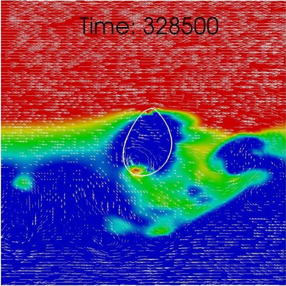
82 Figure 21: Flow around bubble in a high shear of s -1 65

83 Recall from Table 6 that the relative velocity of the s -1 approximately 0.2 m/s, whereas the relative velocity of the 470 s -1 shear case was shear case was approximately 0.34 m/s. For the same surface tension used in each case (0.074 N/m), it is clear that a larger shear rate and higher relative velocity cause the bubble to deform and flatten out. It is thus expected and confirmed for a bubble whose shape is deformed, as seen in Figure 21, the drag coefficient is larger. The drag coefficient correlation (Tomiyama et al., 1998) was developed for a spherical bubble and highly underestimates the extracted values from the high shear simulations, mostly due to bubble deformability, bubble-vortical structure interaction, and velocity flow field around bubble. Another drag coefficient correlation (Ishii & Chawla, 1979) developed for a clean, spherical bubble (function only of bubble Reynolds number) agrees much better with the extracted values seen in Table 21; however, for the shear 470 s -1 case the clean bubble correlation underestimates the extracted value significantly due to a large degree of bubble deformability. A drag coefficient correlation developed for a distorted bubble (function of bubble Reynolds number and surface tension) (Ishii & Chawla, 1979) largely over predicts the extracted value for the shear 470 s -1 case where the bubble became distorted, and under predicts the shear 236 s -1 case extracted value, where the bubble was mainly spherical. For high shear rates, it is difficult to estimate a single parameter, such as Eo or Re bub, to use for comparison with empirical correlations because the high shear rate produces largely varying relative velocities across the bubble which cause largely varying drag forces experienced by the bubble as well as largely varying values of curvature. 66

84 An important concern to address here for the 470 s -1 shear case is the bubble s cross sectional area projected onto the plane normal to the direction of flow. For every drag coefficient calculation, A in Equation ( 41 ) was taken to be the area of a circle with diameter equal to the bubble s initial diameter (1 mm for the 470 s -1 shear case). It is clear from Figure 21 that the bubble s projected area cannot be treated as a perfect circle. However, it is assumed that the true projected area can be approximated by the area of a circle. To obtain the real value of the projected area, an in-simulation advanced analysis of bubble deformation/shape will be required. It is observed that the lift coefficient for the higher shear, higher relative velocity case is also larger than for the lower shear, lower relative velocity case. It has been reported that the lift coefficient has such a strong dependence on the Eötvös number for large bubbles, whom can be easily deformed, that the lift coefficient can become negative (for Eo>6) (Tomiyama et al., 2002). The lift coefficient obtained for the shear 470 s -1 case is observed to be the largest despite the deformed shape of the bubble. It is noted that the semi-empirical lift coefficient correlation (Legendre & Magnaudet, 1998) was developed for spherical bubbles; thus, great agreement was observed between this and the extracted values in Table 22. However, for the higher shear of 470 s -1, where the bubble became deformed, the semiempirical lift coefficient correlation (Legendre & Magnaudet, 1998) under predicted the extracted value. The lift coefficient correlation for high viscosity fluids (Tomiyama et al., 2002) largely under predicts the extracted simulation values where air-water properties were simulated. 67

85 To maintain low relative velocities for high shear rates, the top and bottom moving wall boundary conditions must move in opposite directions. As such, a planar area of zero velocity rests somewhere in the domain depending on desired velocity profile and centerline velocity value. To ensure this area of zero velocity (i.e. point at which drag force flips signs) remained away from the bubble, the prescribed velocity profile on the inflow/outflow boundaries was chosen such that the zero velocity area was below and well away from the bubble. Naturally, the region of zero velocity spawned vortices that were observed to migrate across the domain below the bubble. Some of these vortices interacted with the bubble and could very well account for the high lift coefficient value estimated for the 470 s -1 shear case. Figure 22 shows what the vortical structure development and interaction with the bubble looked like for the 470 s -1 shear case. 68

86 Figure 22: Vortical structure interaction with bubble for shear rate of 470 s -1 69

87 The estimation of the drag and lift coefficients from Table 21 and Table 22 were influenced by several factors: 1) vorticities interacting with bubble, 2) disturbed velocity profile around the bubble, 3) relative velocity definition (liquid velocity value), and 4) bubble deformability. Some of the correlations found in literature have predicted values that are in agreement with the coefficients extracted from the DNS simulations; however, due to the complexity of high shear flows, correlations which accurately predict lift and drag coefficients will need to account for the largely varying velocity profile across the bubble and the implications which it creates (vorticity interactions, disturbed velocity fields, etc.) High shear turbulent cases The high shear turbulent cases proved to be the most difficult control problem reported in this study. Due to the nature of bubble-turbulence interaction, the control forces oscillated much more erratically than for low shear laminar cases; however, the simulations were run long enough to qualitatively observe bubble location and velocity stability such that the temporal averaging of the lift and drag coefficients could be considered statistically steady state. The numerics of high shear turbulent flows also became of concern when the interface became too sharply deformed. The sharp interface deformation experienced in the high shear 236 s -1 turbulent case, caused by bubble-turbulence interactions, resulted in level set divergence and could only be mitigated by temporarily increasing the surface tension. In the high shear 470 s -1 case, another form of numerical divergence was discovered; gas recirculation inside the bubble close to the interface. To mitigate this issue, the gas viscosity was temporarily increased. 70

88 The results, presented in Table 23 and Table 24, were extracted from the high shear turbulent flows of 236 s -1 and 470 s -1. No agreement is found with the predictions by the correlations. Table 23: Estimated drag coefficients for high shear turbulent cases Shear Turbulent 236 Turbulent 470 C d F C d13f C d14f Table 24: Estimated lift coefficients for high shear turbulent cases Shear Turbulent 236 Turbulent 470 C l C l15f As mentioned before, the major concern with the results from the high shear turbulent simulations was due to numerical issues High turbulent shear 236 s -1 discussion The interface, during certain periods of time, became heavily deformed creating a sharp point of curvature. As a result, the level set interface tracking method diverged, rendering the simulation useless. To overcome these periods of sharp interface deformation, the surface tension was temporarily increased allowing for the interface to smooth back out. 13 The value presented here was obtained by ignoring the data at time steps where the relative velocity attained a value of 0 m/s. Refer to Table 25 and Table 26 for discussion about how this value was computed. 14 An empirical drag coefficient correlation for a clean bubble (Ishii & Chawla, 1979) 15 An empirical drag coefficient correlation for a distorted bubble (Ishii & Chawla, 1979) 16 A semi-empirical correlation based on numerical and theoretical solutions (Legendre & Magnaudet, 1998) 71

89 The temporary increase in surface tension led to the bubble attaining a stream-wise velocity equal to the liquid velocity at the location of the bubble resulting in a zero relative velocity. Computation of the instantaneous lift and drag coefficient when the relative velocity takes near zero values results in a non-defined number due to the division by zero. Figure 23 shows the relative velocity of the bubble as a function time. Slightly after 0.2 seconds, around 0.4 seconds, and slightly after 0.5 seconds the relative velocity either attains a zero value or comes very close to doing so. This corresponds to the instances in the simulation when the surface tension was temporarily increased to overcome sharp interface divergence. Velocity (m/s) Time(s) Figure 23: Relative velocity as a function of time for the high shear turbulent 236 s -1 case 72

90 During the lift and drag coefficient computation process, the data corresponding to the times in Figure 23 where the relative velocity approached zero was ignored. There were two ways this was done, automatically and manually. The first way (i.e. automatic way) was a simple average over the whole simulation. At each point in time, when the absolute value of the relative velocity exceeded a minimum limit, this data point was thrown out. This way was run three times with three different minimum relative velocity limits in order to assess sensitivity, see Table 25. The second way (i.e. manual way) was done by manually choosing the time intervals over which to average, see Table 26. Table 25: Lift and drag coefficients for high shear turbulent 236 s -1 case implementing minimum v rel limit Minimum v rel limit (m/s) C d C l Table 26: Lift and drag coefficients for high shear turbulent 236 s -1 case manually choosing temporal averaging interval Time Range (s) C d C l Average of all Time Ranges

91 Agreement can be found between the results presented in Table 25 and Table 26. However, it is clear that the estimation of the lift and drag coefficient is quite sensitive to v rel limit values as well as the temporal average range. Furthermore, the final averages over all the time ranges seen in Table 26 are consistent with the coefficients obtained using the automatic relative velocity limiting average. Figure 24 shows the position and velocity plots for the bubble being simulated in a high turbulent shear of 236 s -1. % Bubble Diameter Velocity (m/s) Bubble X Position Time (s) Bubble X Velocity Time (s) % Bubble Diameter Velocity (m/s) Bubble Y Position Time (s) Bubble Y Velocity Time (s) % Bubble Diameter Velocity (m/s) Bubble Z Position Time (s) Bubble Z Velocity Time (s) Figure 24: Bubble position and velocity plots for high turbulent shear 236 s -1 It is clear from Figure 24 that even though the bubble is well controlled for the majority of the simulation, the times at which the surface tension had to be increased to combat the sharp interface divergence, the bubble became relatively ill controlled. For 74

92 instance, when the surface tension was increased, the bubble s x-velocity (i.e. stream-wise velocity) increased allowing relative velocity to approach small values close to zero. The control force plots, seen in Figure 25, also show the same behavior. x 10-4 X Control Force x 10-4 Y Control Force x 10-5 Z Control Force Force (N) -1 Force (N) 0-2 Force (N) Time (s) Time (s) Time (s) Figure 25: Control force as a function of time for high turbulent shear of 236 s -1 Figure 25 shows the erratic control behavior due to bubble-turbulence interaction. The y-component of the control force clearly shows inconsistency during the times the surface tension had to be increased. Figure 26 shows the time evolution of the bubble being controlled in the high turbulent shear. It is noted that after time step 320,950, up until time step 321,150, the surface tension was increased by a factor of 6.75 to stop the interface from bending sharply. 75

93 Figure 26: Time evolution of a bubble in a high turbulent shear of 236 s -1 76

94 The last three images of Figure 26 show how the bubble shape is quickly altered by the increase in surface tension High turbulent shear 470 s -1 discussion There are several differences between the turbulent shear case of 470 s -1 compared to the turbulent shear case of 236 s -1, namely: relative velocity, bubble Reynolds number, turbulent kinetic energy, and surface tension. As seen in Figure 28, the higher shear, higher relative velocity flow produces many more turbulent structures with larger kinetic energy than that of the lower shear 236 s -1 case. As a result, the chance of sharp interface divergence is much larger in such a turbulent flow, thus throughout the whole 470 s -1 shear simulation, the surface tension value was chosen to be 0.5 N/m (about 6.75 times larger than air-water at standard conditions). It is clear from Figure 28 that the bubble never deforms. Furthermore, because surface tension was always constant in this simulation, the relative velocity remained quasi-constant and never attained zero values, as seen in Figure Velocity (m/s) Time(s) Figure 27: Relative velocity as a function of time for high turbulent shear of 470 s -1 77

95 Figure 28: Time evolution of a bubble in a high turbulent shear of 470 s -1 78

96 Since the relative velocity remained stable during the whole simulation, the lift and drag coefficient computation, as seen in Table 23 and Table 24, was much more straight forward than for the turbulent shear 236 s -1 case. As mentioned before, there was one point during the simulation where the gas velocity inside the bubble diverged. The density of the gas is much less than the liquid density. High turbulence intensity in the liquid can transfer a lot of momentum to the gas inside the bubble. This momentum can result in very high gas recirculation velocities and cause the divergence of the code. To mitigate this recirculation, the gas viscosity was temporarily increased by a factor of 10. The increase in viscosity for this brief amount of time had no visible effect on the bubble controller and the bubble remained well controlled throughout the whole simulation, as seen in Figure 29 and Figure 30. Bubble X Position Time (s) Bubble X Velocity Time (s) % Bubble Diameter Velocity (m/s) % Bubble Diameter Velocity (m/s) Bubble Y Position Time (s) Bubble Y Velocity Time (s) Velocity (m/s) % Bubble Diameter Bubble Z Position Time (s) Bubble Z Velocity Time (s) Figure 29: Bubble position and velocity plots for the high turbulent shear 470 s -1 case 79

97 x 10-4 X Control Force Y Control Force x x 10-4 Z Control Force Force (N) -2-3 Force (N) Force (N) Time (s) Time (s) Time (s) Figure 30: Bubble control force as a function of time for the high turbulent shear 470 s -1 case None of the correlations agree with the coefficients estimated for this high turbulent shear rate and surface tension value. Nevertheless, the result presented here gives insight into high turbulent shear bubble control as well as it provides a numerically estimated value for the lift and drag coefficient of a spherical bubble in a high turbulent shear flow of 470 s Domain Size Study Results A 50% larger domain (in each direction) was run to assess lift and drag coefficient dependence on domain size. However, due to the increase in computational costs, only one large domain case was simulated. A shear rate of 20 s -1 was chosen for a 1 mm bubble. Table 27 shows the estimate drag and lift coefficients for the normal and large sized domain. 80

98 Table 27: Drag and lift coefficients estimated for normal and large size domain with shear rate of 20 s -1 Domain Size Normal Large C d C l Good agreement is observed between lift coefficients of each domain size case as well as between drag coefficients. Both lift and drag coefficient values obtained for the large domain case are within 3% of the normal sized case. Considering the flow for a shear rate of 20 s -1 is relatively calm, the influence on domain size appears to be negligible. However, a domain size study for higher shear rates will be required to determine whether or not this parameter can influence lift and drag coefficient estimation, especially as the flow becomes more erratic and vortical structures begin to interact with the bubble. 81

99 Figure 31: Steady state flow for large domain case, shear 20 s PWR Fluid Properties Cases One of the goals of this study was to provide a path forward to simulating full-fledged reactor conditions. In order to do so, simple cases (low shear rates) must be run first to observe flow and bubble behavior and more importantly assess the bubble control algorithm performance. Table 28 and Table 29 show the estimated drag and lift coefficients for the PWR fluid properties simulations. 82

100 Table 28: Estimated drag coefficients for shear rates 20 s -1 and 100 s -1 with PWR saturated fluid properties Shear Rate (s -1 ) C d C d16f C d17f Table 29: Estimated lift coefficients for shear rates 20 s -1 and 100 s -1 with PWR saturated fluid properties Shear Rate (s -1 ) C l C l18f Good agreement is found between the shear 20 s -1 estimated drag coefficient and the two correlations (one for clean bubble and the other for distorted bubble). Recall that the bubble Reynolds number for this case is about 800. No agreement is found between the estimated lift coefficient and the correlation; however, the estimated lift coefficient does follow a certain, widely recognized trend, that is, as the bubble becomes deformed, the lift coefficient approaches zero and then flips signs (this phenomena is observed in bubbly flow experiments as the wall peaking void fraction profile for small spherical bubbles, and centerpeaking void fraction profile for larger deformable bubbles). Figure 32 displays the steady state flow and bubble behavior for the shear rate of 20 s -1. For the shear 100 s -1 case, no agreement is found between the estimated values and the correlations. 17 An empirical drag coefficient correlation for a clean bubble (Ishii & Chawla, 1979) 18 An empirical drag coefficient correlation for a distorted bubble (Ishii & Chawla, 1979) 19 A semi-empirical correlation based on numerical and theoretical solutions (Legendre & Magnaudet, 1998) 83

101 Figure 32: Steady state flow for the shear rate of 20 s -1 using PWR saturated fluid properties It can be seen from Figure 32 that the wake has a large influence on the estimated lift coefficient. Directly behind the bubble (east side) in its wake, a large recirculation region exists where flow is moving north. The result of the slanted wake in addition to the slight deformation observed causes the lift coefficient to be very small. Essentially, the wake behavior for this case acts against the lift force and causes the estimated lift coefficient to be the smallest. Figure 33 shows how the y-component of the control force is very small, as it fluctuates close to zero, thus proposing a small acting lift force. 84

102 X Control Force x x Y Control Force 1.5 x 10-8 Z Control Force Force (N) Force (N) -1-2 Force (N) Time (s) Time (s) Time (s) Figure 33: Control force as a function of time for the shear 20 s -1 case with PWR saturated fluid properties Figure 34 shows how the control force behaves as a function of time for the higher shear PWR fluid properties case. Currently, the bubble controller is not well converged as it is in Figure 33. A longer simulation run for the shear 100 s -1 case will be required to ensure statistically steady state values. 85

103 x X Control Force Y Control Force x x Z Control Force Force (N) -4-5 Force (N) Force (N) Time (s) Time (s) Time (s) Figure 34: Control force as a function of time for the shear 100 s -1 case with PWR saturated fluid properties Figure 35 shows the flow field around the bubble in a shear rate of 100 s -1. It is obvious that the high shear flow embodies much more energy than the low shear flow, and hence bubble-turbulence interaction plays a large role in the estimation of the lift and drag coefficients. The velocity profile around the bubble is observed to be distorted owing to a larger lift coefficient estimation than in the low shear PWR fluid properties case. 86

104 Figure 35: Flow around bubble for the shear rate of 100 s -1 using PWR saturated fluid properties 3.9 Computational Costs Estimate Computational costs are important to estimate in order to assess simulation throughput efficiency. Ideally, one would desire to obtain statistically steady state results at the quickest rate to maximize work flow. However, computational hardware limits the throughput rate. The following section will briefly estimate the computational costs for a couple of results presented in this work. 87

105 Table 30 shows the CPU-hour estimate for several cases presented in this research. Table 31 shows the total amount of CPU-hours in a single week for the HPC machine, Insight, which was used to complete this research. Insight is a local, high performance computer consisting of 1 head master node and 6 compute nodes, each with four 16-core AMD Operton TM 6000 series processors (64 cores per node). Each compute node contains 128 GB of DDR MHz ECC RDIMM memory. Open source LINUX is the operating system. Table 30: CPU-hour estimate for shear 50 s -1 (laminar), 100 s -1 (laminar), 236 s -1 (laminar and turbulent) Case Shear 50 Shear 100 Shear 236 (L) Shear 236 (T) Total Simulation Time (s) Total Number of Time steps 30, , , ,950 Total Wall Clock Time (hr) Number of Cores Total Number of Mesh Elements 500, , , ,000 CPU-Hours Estimate 3, , , ,899.2 Table 31: Total CPU-hour for a single week on Insight HPC machine Number of Cores 384 Total CPU-hours for a Single Week 64,512 88

106 The total number of CPU-hours for a single week, assuming 100% computing capacity that Insight contains is approximately 64.5 thousand. The turbulent shear cases take the longest to run due to core-domain allocation (time varying boundary condition data is handled by one core). This means that if 100% of Insight s cores could be used at 100% capacity, almost 3 turbulent shear cases, similar to the 236 s -1 case, could be run in a single week. However, to increase this throughput, code modification/optimization will need to be done to allow for more cores to be utilized for a turbulent shear case. Currently, 64 is the recommended number of cores that can be used to successfully run a turbulent shear case due to the serial nature of the time-varying-type boundary condition used to feed the turbulent flow into the two-phase simulation domain. Thus, each case required about 2 weeks of run time, but up to 6 cases could be run with the currently available machine. Migrating to HPC would allow many more cases to be run in parallel. 89

107 4. CONCLUSIONS The results presented in this thesis have built a foundation in which the lift and drag coefficients for high shear laminar and turbulent flows can be estimated. While the estimated values are in relatively good agreement with predictions acquired by empirical and semiempirical correlations, the results presented herein have provided an outlook for developing state-of-the-art lift and drag correlations for high shear flows. Some general conclusions achieved from this research are: 1. The majority of current lift and drag correlations are for low shear, laminar flows. Application of these correlations in CMFD codes, which simulate reactor conditions, may not be the most accurate. 2. A method has been developed for estimating the shear-induced lift force on a single bubble in laminar and turbulent shear flows using direct numerical simulation coupled with interface-tracking methods. State-of-the-art correlations for high shear flows can be developed to complement the existing database. 3. The low shear laminar flow results presented in this paper have shown agreement with current correlations and offer assurance that the bubble control method developed as a part of this thesis is credible. 4. Transition to simulating higher shear rates has been accomplished by simulating a number of medium shear laminar flows. The result has provided a qualitative understanding of how the flow field around the bubble changes with increasing shear rate. Vortical structures have been observed to develop and interact with the bubble when simulating a high shear rate with low relative velocity. Current 90

108 correlations offer a basis for comparison, but none account for flow field disturbance and bubble-turbulence interaction. 5. High shear laminar flows have been simulated to discover that the flow doesn t remain predominantly laminar, and that turbulent vorticities develop around the region of zero liquid velocity due to the high shear. The vorticities then interact with the bubble influencing the estimation of the drag and lift coefficients. No correlations have been found which predict lift and drag coefficients at such high shear rates. 6. High shear turbulent flow simulations have also been conducted to observe bubble-turbulence interaction. The PID-based controller was observed to be much more erratic while trying to reduce bubble motion. Due to unstable numerical issues for increasing shear rates, such as sharp interface deformation/divergence and gas recirculation divergence, the surface tension and gas viscosity had to be increased temporarily. Increasing the surface tension resulted in zero instantaneous relative velocity values. When the relative velocity became zero, the lift and drag data had to be ignored. Increasing the gas viscosity had no visible effect on the bubble controller or lift and drag estimation. Averaging over the fluctuations caused by bubble-turbulence interaction allowed for estimation of the lift and drag coefficients for two high turbulent shear rates of 236 s -1 and 470 s PWR fluid properties were simulated with low to medium shear flows to assess initial bubble controller performance. The difference in flow for the lower and higher shear cases deviated significantly. For the low shear case, the lift 91

109 coefficient was especially small due to bubble-wake interaction and slight deformation. For the higher shear case, the flow field around the bubble was distorted and vortical structures were generated due to high flow energy causing bubble-turbulence interaction. It was found that the bubble controller performed well under the low-density/low-viscosity ratio conditions. The control algorithm is expected to perform better for increasing shear flows and even turbulent flows because the density and viscosity ratios corresponding to PWR fluid properties are much more numerically stable than high density/high viscosity flows. 8. An advance in computing capacity can open up new doors for the simulations reported herein. For instance, larger domains with larger meshes can be developed to ensure boundary conditions do not influence flow physics and bubble movement. 9. The thesis work provides an excellent foundation for which high shear, high Reynolds number, turbulent, complex geometry simulations can build upon. Direct numerical simulations coupled with the level set interface tracking method have proved to be a valuable tool when coupled with high performance computing for estimating the shear induced lift force on a single bubble. To ensure a successful transition to the widespread use of CMFD in the design of future nuclear reactors, where safety is the number one goal, it is crucial to further develop and validate the current thermal-hydraulic models with state-of-the-art techniques. The innovative method and novel results presented in this paper can be used to complement the existing analytical, numerical, and experimental lift correlation database. 92

110 4.1 Future Work In order to increase the fidelity of the method developed as a part of this research and expand upon the data obtained, suggestions for further work will be made in this section. A major concern with estimating the lift and drag coefficient for a single bubble in high shear flows is the definition of the relative velocity, or more specifically, how does one define the value of the liquid velocity which is moving relative to the bubble velocity? At low shears, the liquid velocity value is simply taken to be the value of the liquid velocity at the location of the bubble s center. It is also known for low shears that the velocity field around the bubble is minimally disturbed relative to large shears where the energetic flow begins to produce vorticities. Thus for low shears, the relative velocity definition using the liquid velocity at the bubble s center is a safe assumption. However, for high shears, when the flow field around the bubble becomes distorted and deviates significantly from the initial flow field, it becomes more challenging to describe the relative velocity. A recommendation for future work is to develop a method for determining representative relative velocities for bubbles in energetic and dynamic flow fields. For example, numerically speaking, the liquid velocities around the near region of the interface can be averaged to obtain a representative relative velocity for the given disturbed flow field that the bubble experiences. It can be shown that for lower shear rates, where the flow is relatively more laminar around the bubble, the average of the liquid velocities around the bubble s interface result in the liquid velocity value at the center of the bubble if the bubble wasn t there. The problem that arises is defining the region around the interface to do the averaging. Larger shear rates which provoke larger vortical structures may need to average over a larger volume. To ensure a 93

111 proper averaging region, studies should be conducted to assess the deviation in average liquid velocity when the averaging is done over different sized regions (and maybe even shapes). It was presented (Tomiyama et al., 2002) that the sum of the shear induced lift force and the slanted wake induced lift force equals the net transverse lift force that a bubble experiences in a shear flow. A recommendation for future work is to quantify the slanted wake induced lift force. The current data base describing the complex interaction between the bubble s wake and the surrounding shear velocity field is insufficient and ought to be improved. It was observed for very high shear rates of laminar flows that vortical structures were produced at the inflow/outflow boundary conditions, which could have influenced the estimated lift and drag coefficients. As such, a large domain study, which utilized a computational domain 50% larger in each direction, was run to assess the influence of the bubble being too close to the inflow/outflow boundaries. However, this study was done for a relatively lower shear rate of 20 s -1, where vortical structures were not seen to develop from the inflow/outflow boundaries. A recommendation for future work is to run a very high shear laminar case (236 s -1 or 470 s -1 ) to assess domain size influence on estimating the lift and drag coefficient. The PWR fluid properties case was run for a low shear of 20 s -1 and 100 s -1. The reason for this was simplicity. In order to simulate increasingly complex flows (e.g. high shear rates and/or turbulence) simple cases must be run first to assess control behavior, and in general, flow behavior. Future work should capitalize on the results obtained from the low medium range shear rates presented in this study utilizing PWR fluid properties. Eventually, 94

112 as the database is built up from running the simple cases, full-fledge reactor coolant conditions can be tackled with enough assurance in control dependability and stability. Another recommendation for the PWR fluid properties cases is to simulate a larger domain. It was observed that the domain sized used in these cases allowed for interaction between the bubble s wake and the prescribed velocity boundary condition. Estimation of the lift and drag forces could be influenced by such an interaction. Thus a larger domain could allow one to assess domain size on the estimation of lift and drag coefficients for the PWR fluid properties cases where the bubble Reynolds numbers are much larger causing the bubble s wake to be longer. The mesh study presented in this report allowed for the observation of something interesting. At the finest mesh resolution, 24 elements across the bubble, small fluctuations in the bubble s trailing wake were detected. As a result, two explanations were hypothesized: a) Small turbulent eddies were resolved in the bubble s wake. The resolution of these eddies allowed for the velocity profile near the interface to be influenced ultimately affecting the estimated lift and drag coefficients. b) Small numerical waves synchronizing with the bubble s wake could be affecting the estimation of the lift and drag coefficients. Further, detailed mesh resolution testing should be completed to determine the likelihood of the two hypotheses presented above. As the shear rate was increased, bubble deformation became more apparent. If the bubble deforms to a certain degree, assuming a circular projected area during the computation of the drag coefficient may introduce more error than desired. A representative 95

113 deformability factor (Fang et al., 2013) can be extracted from the simulation to assess a better estimation of the bubble s true projected area. Perhaps an algorithm for projecting the bubble s shape onto a plane normal to the flow can be developed for the most accurate assessment of projected area and thus an estimation of the drag coefficient with the least amount of error introduced by the projected area calculation. More turbulent cases can be run to expand upon the results obtained in this research work. It was noted for the 236 s -1 turbulent shear case that bubble deformation caused the divergence of the simulation and led to the need to temporarily increase surface tension. For the 470 s -1 turbulent shear case, surface tension remained constant at a larger-than-normal value to overcome bubble deformation divergence. Using the surface tension value from the 470 s -1 turbulent shear case, the 236 s -1 turbulent shear case should be re-run to assess differences in the estimated lift and drag coefficients between these two cases. For higher shear rates, where bubble-turbulence interaction became important, it was noted that the functional form of the lift and drag force (Equations ( 13 ) and ( 16 )) may be insufficient in describing the associated phenomena. It is recommended that lift and drag force functions be studied to ensure and perhaps develop the best functional form, especially for bubbles in high turbulent shear flows. The new model would account for non-linear effects observed in the virtual experiments. A practical next step for this research includes the study of the lift force behavior in a multiple bubble flow. Two strategies are recommended for this: 96

114 1. Simulate single bubble in shear flow with periodic boundary conditions to replicate a train of bubbles. The width of the domain can be varied to assess influence of the spacing of bubbles in a train. 2. Control a single bubble in a shear flow where multiple bubbles flow around it. This will enable one to estimate the lift force on a single bubble in a bubble cluster. An implication resulting from computational expense constraints in this research work was the necessity of controlling the stream-wise movement of the bubble. A longer domain (thus a more expensive domain) could allow for the need to only control the lateral movement of the bubble (thus only extracting lift coefficients). This could further allow for the ability to simulate a bubble in liquid velocities more like that seen in a PWR coolant channel. Also, it could allow for the testing of Galilean invariance, which states that the laws of motion are the same in all inertial reference frames. The estimation of the lift and drag coefficients for a bubble with no relative motion may be different when the bubble is allowed to flow through the domain. The method developed in this research for estimating the lift and drag coefficients on a bubble in a shear flow should be extensively verified and validated. For simulations which involved bubble-turbulence interaction, one might claim that the numerical method is not full DNS due to interaction of the level set interface with the turbulence itself. DNS is a numerical method for solving the Navier-Stokes equations without any turbulence model by fully resolving all scales of turbulence. The question then arises: is the turbulence interaction with interface leading to bubble deformation physical and is the turbulent kinetic energy transfer through interface physical for high Reynolds number 97

115 flows? Validation and verification of bubble-turbulence interaction and bubble deformability should be pursued to ensure results are the most accurate. The current results presented herein may also be questioned about whether the mesh resolution around the interface was sufficient for resolving bubble induced turbulence. Appendix E provides a calculation of the y + values adjacent to the inner and outer side of the interface for shear rates of 110 s -1 and 236 s -1. The current mesh resolutions provide confidence in the estimations of lift and drag for shear rates of 110 s -1 and below. For shear rates of 236 s -1 and above, the current mesh resolution may require refinement in order to ensure appropriate bubble induced turbulence resolution. Due to the serial nature of the time-varying-type boundary condition, which was used in the turbulent two-phase cases, only a single processor handled both inflow/outflow planes. For a 535,000 element mesh run on 128 processors, each processor was assigned about 4,180 elements. The two inflow/outflow boundary condition planes, together, consisted of 10,700 elements. Where the majority of processors had to do computation for 4,180 elements, one processor had to do computation for more than twice this amount. In addition, message passing interface (MPI) requires much more communication through these boundary planes and processor load is at a greater unbalance, thus slowing down throughput significantly. It is highly recommended that the serial nature of the time-varying-type boundary condition function in PHASTA be made parallel in order to increase turbulent case throughput. 98

116 REFERENCES Auton, T. R. (1987). The lift force on a spherical body in a rotational flow. Journal of Fluid Mechanics, 183, Bolotnov, I. A. (2013). Influence of bubbles on the turbulence anisotropy. Journal of Fluids Engineering, Bolotnov, I. A., Jansen, K. E., Drew, D. A., Oberai, A. A., & Lahey, R. T. (2011). Detached direct numerical simulation of turbulent two-phase bubbly channel flow. International Journal of Multiphase Flow, 37, Brackbill, J. U., Kothe, D. B., & Zemach, C. (1992). A continuum method for modeling surface tension. Journal of Computational Physics, 100(2), Cherukat, P., & McLaughlin, J. B. (1994). The inertial lift on a rigid sphere in a linear shear flow field near a flat wall. Journal of Fluid Mechanics, 263, De Chant, L. J. (2005). The venerable 1/7th power law turbulent velocity profile: A classical nonlinear boundary value problem solution and its relationship to stochastic processes. Applied Mathematics and Computation, 161, Drew, D. A., & Lahey, R. T. (1987). The virtual mass and lift force on a sphere in rotating and straining inviscid flow. International Journal of Multiphase Flow, 13,

117 Drew, D. A., & Passman, S. L. (1998). Theory of multicomponent fluids. New York: Springer. McGuire nuclear generation station, Updated Final Safety Analysis ReportU.S.C. Chapter 4 (2003). Ervin, E. A., & Tryggvason, G. (1997). The rise of bubbles in a vertical shear flow. Journal of Fluids Engineering, 119, Esmaeeli, A., & Tryggvason, G. (2004). Computations of film boiling. part I: Numerical method. International Journal of Heat and Mass Transfer, 47, Fang, J., Lu, J., Thomas, A. M., Bolotnov, I. A., & Tryggvason, G. (2013). ITM/DNS database of drag, lift and wall effects, including the effects of void fractions. (CASL Milestone Report No. 1.7). Fang, J., Thomas, A. M., & Bolotnov, I. A. (2013). Development of advanced analysis tools for interface tracking simulations. Transactions of the 2013 ANS Winter Meeting, Washington D.C. Giusti, A., Lucci, F., & Soldati, A. (2005). Influence of the lift force in direct numerical simulation of upward/downward turbulent channel flow laden with surfactant contaminated microbubbles. Chemical Engineering Science, 60(22), doi: 100

118 Haberman, W. L., & Morton, R. K. (1953). An experimental investigation of the drag and shape of air bubbles rising in various liquids. (David W Taylor Model Basin No. 802).United States Navy Department. Hibiki, T., Goda, H., Kim, S., Ishii, M., & Uhle, J. (2004). Structure of vertical downward bubbly flow. International Journal of Heat and Mass Transfer, 47, Hibiki, T., & Ishii, M. (1999). Experimental study on interfacial area transport in bubbly twophase flows. International Journal of Heat and Mass Transfer, 42, Hibiki, T., & Ishii, M. (2007). Lift force in bubbly flow systems. Chemical Engineering Science, 62, Hibiki, T., Ishii, M., & Xiao, Z. (2001). Axial interfacial area transport of vertical bubbly flows. International Journal of Heat and Mass Transfer, 44, Hibiki, T., Situ, R., Mi, Y., & Ishii, M. (2003). Local flow measurements of vertical upward bubbly flow in an annulus. International Journal of Heat and Mass Transfer, 46, Ishii, M., & Chawla, T. C. (1979). Local drag laws in dispersed two-phase flow. Argonne National Laboratory Report, ANL (NUREG/CR-1230), 101

119 Jansen, K. E. (1993). Unstructured grid large eddy simulations of wall bounded flows. Annual Research Briefs, Center for Turbulence Research, NASA Ames/Stanford University,, 151. Jansen, K. E. (1999). A stabilized finite element method for computing turbulence. Computer Methods in Applied Mechanics and Engineering, 174, Juric, D., & Tryggvason, G. (1998). Computations of boiling flows. International Journal of Multiphase Flow, 24(3), Kariyasaki, A. (1987). Behavior of a gas bubble in a liquid flow with a linear velocity profile. Transactions of Japan Society of Mechanical Engineers, B(53), Lahey, R. T. (2005). The simulation of multidimensional multiphase flows. Nuclear Engineering and Design, 235, Legendre, D., & Magnaudet, J. (1998). The lift force on a spherical bubble in a viscous linear shear flow. Journal of Fluid Mechanics, 368, Liu, T. J. (1993). Bubble size and entrance length effects on void development in a vertical channel. International Journal of Multiphase Flow, 19(1), Lu, J., & Tryggvason, G. (2006). Numerical study of turbulent bubbly downflows in a vertical channel. Physics of Fluids, 18,

120 Magnaudet, J., & Mougin, G. (2007). Wake instability of a fixed spheroidal bubble. Journal of Fluid Mechanics, 572, Marie, J. L. (1987). Modelling of the skin friction and heat transfer in turbulent twocomponent bubbly flows in pipes. International Journal of Multiphase Flow, 13, Mazzitelli, I. M., & Lohse, D. (2003). The effect of microbubbles on developed turbulence. Physics of Fluids, 15(1), L5-L8. doi:0.1063/ Mazzitelli, I. M., Lohse, D., & Toschi, F. (2003). On the relevance of the lift force in bubbly turbulence. Journal of Fluid Mechanics, 488, doi: /s Nagrath, S. (2004). Adaptive stabilized finite element analysis of multi-phase flows using a level set approach. (Ph.D., Rensselaer Polytechnic Institute). Nagrath, S., Jansen, K. E., Lahey, R. T., & Akhatov, I. (2006). Hydrodynamic simulation of air bubble implosion using a FEM based level set approach. Journal of Computational Physics, 215, NASA. (2010). Drag of a sphere. Retrieved, 2014, Retrieved from 103

121 Pascal, P., & Oesterlé, B. (2000). On the dispersion of discrete particles moving in a turbulent shear flow. International Journal of Multiphase Flow, 26(2), doi: Saffman, P. G. (1965). The lift on a small sphere in a slow shear flow. Journal of Fluid Mechanics, 22(2), Saffman, P. G. (1968). Corrigendum to The lift on a small sphere in a slow shear flow. Journal of Fluid Mechanics, 31, 624. Sahni, O., Mueller, J., Jansen, K. E., Shephard, M. S., & Taylor, C. A. (2006). Efficient anisotropic adaptive discretization of the cardiovascular system. Computer Methods in Applied Mechanics and Engineering, 195(41-43), Segré, G., & Silberberg, A. (1962a). Behaviour of macroscopic rigid spheres in poiseuille flow. part 1. Journal of Fluid Mechanics, 14, Segré, G., & Silberberg, A. (1962b). Behaviour of macroscopic rigid spheres in poiseuille flow. part 2. Journal of Fluid Mechanics, 14, Sene, K. J., Hunt, J. C. R., & Thomas, N. H. (1994). The role of coherent structures in bubble transport by turbulent shear flows. Journal of Fluid Mechanics, 259, Serizawa, A., & Kataoka, I. (1994). Dispersed flow I. Multiphase Science and Technology, 8,

122 Sethian, J. A. (1999). Level set methods and fast marching methods Cambridge University Press. Sridhar, G., & Katz, J. (1995). Drag and forces on microscopic bubbles entrained by a vortex. Physics of Fluids, 7, Sridhar, G., & Katz, J. (1999). Effect of entrained bubbles on the structure of vortex rings. Journal of Fluid Mechanics, 397, 171. Sussman, M., Almgren, A. S., Bell, J. B., Colella, P., Howell, L. H., & Welcome, M. L. (1999). An adaptive level set approach for incompressible two-phase flows. Journal of Computational Physics, 148(1), Sussman, M., & Fatemi, E. (1999). An efficient, interface-preserving level set re-distancing algorithm and its application to interfacial incompressible fluid flow. Siam Journal on Scientific Computing, 20(4), Sussman, M., Fatemi, E., Smereka, P., & Osher, S. (1998). An improved level set method for incompressible two-phase flows. Journal of Computers & Fluids, 27(5-6), Takagi, S., & Matsumoto, Y. (1995). Three dimensional calculation of a rising bubble. Proceedings of the Second International Conference on Multiphase Flow, Kyoto, Japan. 105

123 Tejada-Martinez, A. E., & Jansen, K. E. (2005). A parametric-free dynamic subgrid-scale model for large-eddy simulation. Computer Methods in Applied Mechanics and Engineering, 194(9), Thomas, A. M., Fang, J., & Bolotnov, I. A. (2014). Estimation of shear-induced lift force in laminar and turbulent flows. Embedded Topical Meeting: Advances in Thermal Hydraulics, Reno, NV. Thomas, A. M., & Bolotnov, I. A. (2012). Evaluating shear induced lift force using interface tracking approach. Transactions of the 2012 ANS Winter Meeting, San Diego, CA. Tomiyama, A. (2004). Drag, lift, and virtual mass forces acting on a single bubble. Proceedings of the Third International Symposium on Two-Phase Flow Modeling and Experimentation, Pisa, Italy. Tomiyama, A., Kataoka, I., Zun, I., & Sakaguchi, T. (1998). Drag coefficients of single bubbles under normal and micro gravity conditions. The Japan Society of Mechanical Engineers, 41(B), Tomiyama, A., Sou, A., Zun, I., Kanami, N., & Sakaguchi, T. (1995). Effects of eötvös number and dimensionless liquid volumetric flux on lateral motion of a bubble in a laminar duct flow. Advances in Multiphase Flow,, Tomiyama, A., Tamai, H., Zun, I., & Hosokawa, S. (2002). Transverse migration of single bubbles in simple shear flows. Chemical Engineering Science, 57,

124 Tomiyama, A., Zun, I., Sou, A., & Sakaguchi, T. (1993). Numerical analysis of bubble motion with the VOF method. Nuclear Engineering and Design, 141, Wang, L., & Maxey, M. R. (1993). The motion of microbubbles in a forced isotropic and homogeneous turbulence. Applied Scientific Research, 51, Wang, S. K., Lee, S. J., Jones, O. C., & Lahey, R. T. (1987). 3-D turbulence structure and phase distribution measurements in bubbly two-phase flows. International Journal of Multiphase Flow, 13(3), Whiting, C. H. (1999). Stabilized finite element methods for fluid dynamics using a hierarchical basis. (Ph.D., Rensselaer Polytechnic Institute). Whiting, C. H., & Jansen, K. E. (2001). A stabilized finite element formulation for the incompressible navier-stokes equations using a hierarchical basis. International Journal of Numerical Methods in Fluids, 35, Zhongchun, L., Xiaoming, S., Shengyao, J., & Jiyang, Y. (2014). Numerical investigation on lateral migration and lift force of single bubble in simple shear flow in low viscosity fluid using volume of fluid method. Nuclear Engineering and Design, 274, Zhou, M., Sahni, O., Jin Kim, H., Figueroa, C. A., Taylor, C. A., Shephard, M. S., & Jansen, K. E. (2010). Cardiovascular flow simulation at extreme scale. Computational Mechanics, 46,

125 Zun, I. (1980). Transverse migration of bubbles influenced by walls in vertical bubbly flow. International Journal of Multiphase Flow, 6, Zun, I. (1988). Transition from wall void peaking to core void peaking in turbulent bubbly flow. Transient Phenomena in Multiphase Flow, Washington D.C

126 APPENDICES 109

127 Appendix A Below is a calculation of approximate reactor environment relative velocities and shear rates using data obtained from Chapter 4 of McGuire Nuclear Power Plant (NPP) updated final safety analysis report (UFSAR) (Duke Energy, 2003). Table 32: VANTAGE+ fuel assembly design for McGuire NPP (Duke Energy, 2003) Rod Pitch (in, m) 0.496, Rod OD (in, m) 0.374, Channel Velocity(ft/s, m/s) , Average Mass Velocity (lbm/hr/ft 2, kg/hr/m 2 ) , Hydraulic Diameter (in, m) 0.464, T ave ( F, K) 587.3, Pressure (psia, bar) 2250, 155 Table 33: Typical fluid properties of a coolant channel T sat@2250psia ( F, K) , ρρ l,sat (lbm/ft 3, kg/m 3 ) , ρρ g,sat (lbm/ft 3, kg/m 3 ) 6.372, F (lbm/ft/hr, kg/m/hr) , F (lbm/ft 3, kg/m 3 ) , g (ft/s 2, m/s 2 ) , 9.81 Bubble Diameter (in, m) , The Reynolds number for a channel is given by: Re = F vv channnnel D h F = ( A. 1 ) 110

128 Assuming that the drag coefficient on a spherical bubble at a Bubble Reynolds number on the order of 10 2 is approximately 1.0 (NASA, 2010), we can calculate a bubble relative velocity from a force balance. A force balance on the bubble moving at a constant velocity up the fuel channel is given by: FF D = 1 2 CC Dρρ l,sat vv r 2 A = FF B = ρρ l,sat ρρ g,sat V b g ( A. 2 ) Solving for relative velocity, v r : vv r = 2 ρρ l,sat ρρ g,sat V b g CC D ρρ l,sat A ( A. 3 ) calculated by: Assuming that a spherical bubble moves through the channel, volume and area are V b = π D bubble 2 ( A. 4 ) A b = π D 2 bubble 2 ( A. 5 ) 111

129 The following table calculates relative velocities for spherical bubble sizes that range from 0.1mm to 0.5mm in diameter. Table 34: Approximate relative velocities of small spherical bubbles in sub-channel D bubble (m) A b (m 2 ) V b (m 3 ) v r (m/s) Re b Using the 1/7 th power law (De Chant, 2005) for obtaining a velocity profile near the wall of a reactor coolant channel, we can determine approximate shear rates also. Since we know the geometry as well as the average velocity in the sub-channel, we can obtain a subchannel velocity profile by solving the following equation: D cc xx 1 hydraulic 7 ddxx 0 = vv D avg,sub channnnel ( A. 6 ) hydrauliic where c is just a coefficient that scales the 1/7 th power law to ensure the average velocity in the channel is that taken from Table 32. It is found that c=9.966, allowing for the velocity in the sub-channel to be defined as: vv sub channnnel (xx) = xx 1 7 ( A. 7 ) 112

130 Figure 36: Mean sub-channel velocity profile in typical PWR coolant channel Figure 36 displays the approximate sub-channel velocity profile according to the 1/7 th power law using parameters from Chapter 4 of McGuire NPP UFSAR (Duke Energy, 2003). The derivative of the velocity profile can be taken in order to get the shear rate as a function of distance from the wall, x. Sr(xx) = dd ddxx vv sub channnnel(xx) = y 6 7 ( A. 8 ) 113

131 Figure 37: Mean shear rate in sub-channel of typical PWR According to Figure 37, the shear rate that a bubble experiences close to the wall of a sub-channel is on the order of 10 3 s -1. Table 35: Approximate shear rate values close to the wall of typical PWR fuel rod Distance From Wall, x, (m) Sr(x) (s -1 ) It is determined that the numerical simulations presented in this study meet the goals of this appendix and provide an excellent stepping stone for future simulations that will simulate even higher turbulent shear rates. 114

132 this paper. Appendix B This appendix contains all control force vs. time plots for every result presented in Figure 38: Control force vs. time: 1.0 s -1 shear, m/s relative velocity, 5 mm bubble Figure 39: Control force vs. time: 2.0 s -1 shear, 0.05 m/s relative velocity, 5 mm bubble 115

133 Figure 40: Control force vs. time: 5.0 s -1 shear, 0.05 m/s relative velocity, 5 mm bubble Figure 41: Control force vs. time: 10.0 s -1 shear, 0.05 m/s relative velocity, 5 mm bubble 116

134 Figure 42: Control force vs. time: 10.0 s -1 shear, m/s relative velocity, 1 mm bubble Figure 43: Control force vs. time: 20.0 s -1 shear, m/s relative velocity, 1 mm bubble 117

135 Figure 44: Control force vs. time: 30.0 s -1 shear, m/s relative velocity, 1 mm bubble Figure 45: Control force vs. time: 40.0 s -1 shear, m/s relative velocity, 1 mm bubble 118

136 Figure 46: Control force vs. time: 50.0 s -1 shear, m/s relative velocity, 1 mm bubble Figure 47: Control force vs. time: 75.0 s -1 shear, m/s relative velocity, 1 mm bubble 119

137 Figure 48: Control force vs. time: s -1 shear, m/s relative velocity, 1 mm bubble Figure 49: Control force vs. time: s -1 shear, m/s relative velocity, 1 mm bubble 120

138 Figure 50: Control force vs. time: s -1 laminar shear, m/s relative velocity, 1 mm bubble Figure 51: Control force vs. time: s -1 laminar shear, m/s relative velocity, 1 mm bubble 121