Dedicated to Major Contributors to the Concepts of Flow of Water and Sediment in Alluvial Channels:

Transcription

1 Geomorphic, Hydrologic, Hydraulic and Sediment Concepts Applied To Alluvial Rivers By Daryl B. Simons, Ph.D., P.E., D.B. Simons & Associates, Inc.; Everett V. Richardson, Ph.D., P.E., Ayres Associates, Inc.; Maurice L. Albertson, Ph.D., P.E., Colorado State University; Robert J. Kodoatie, Ph.D., Diponegoro University, Indonesia Daryl B. Simons Published by Colorado State University OPEN FILE INTERNET FREE DOWNLOAD

2 Dedicated to Major Contributors to the Concepts of Flow of Water and Sediment in Alluvial Channels: Paul C. Benedict, U.S. Geological Survey; Donald C. Bondurant, U.S. Corps of Engineers; Whitney M. Borland, U.S. Bureau of Reclamation; Bruce R. Colby, U.S. Geological Survey; Brynon C. Colby, U.S. Geological Survey; Hans A. Einstein, University of California, Berkeley; Dave W. Hubbell, U.S. Geological Survey; E.W. Lane, U.S. Bureau of Reclamation; Emmett M. Laursen, University of Arizona; Luna B. Leopold, U.S. Geological Survey; Carl F. Nordin, U.S. Geological Survey; Hunter Rouse, University of Iowa; Stanley E. Schumm, Colorado State University; Lorenzo G. Straub, University of Minnesota; and Vito A. Vanoni, California Institute of Technology.

3 iii Table of Contents LIST OF SYMBOL... V ABSTRACT... IX 1. INTRODUCTION FUNDAMENTALS THAT MUST BE INTEGRATED INTO THE TRANSPORT ANALYSIS OF AN ALLUVIAL CHANNEL ALLUVIAL GEOMORPHOLOGY REGIMES OF FLOW AND BEDFORMS IN ALLUVIAL CHANNELS Bed Configuration Plane Bed Without Sediment Movement Ripples Dunes Plane Bed With Movement Antidunes Chutes and Pools Regime of Flow, Configuration, and Froude Number Bars GEOMORPHIC RELATIONS THAT ASSIST PRELIMINARY ANALYSIS OF ALLUVIAL CHANNELS APPLICATIONS OF GEOMORPHIC AND HYDROLOGIC ANALYSIS DATABASE THE THREE-LEVEL ANALYSIS OF ALLUVIAL RIVERS RESISTANCE TO FLOW IN ALLUVIAL RIVERS CLASSIFICATION OF OPEN CHANNELS VARIATION OF MANNING S RESISTANCE COEFFICIENT FOR ALLUVIAL CHANNELS FORM ROUGHNESS SELECTING ROUGHNESS COEFFICIENTS FOR A PRACTICAL CASE DATA REQUIRED TO ESTIMATE MANNING'S N, VELOCITY, STAGE, AND SEDIMENT TRANSPORT Data Required for Alluvial Channels Data Required for the Floodplain CONCEPTS TO REMEMBER BEGINNING OF MOTION INTRODUCTION REPRESENTATIVE DIAMETER OF A BED-MATERIAL MIXTURE... 37

4 4.3 THEORETICAL CONSIDERATIONS THEORY OF BEGINNING OF MOTION EXPERIMENTAL APPROACHES SHIELDS DIAGRAM OTHER FORMULAE DEFINING THE BEGINNING OF MOTION APPLICATION OF BEGINNING OF MOTION TO PRACTICAL PROBLEMS SEDIMENT TRANSPORT HISTORIC NOTE FUNDAMENTALS OF SEDIMENT TRANSPORT SUSPENDED BED SEDIMENT DISCHARGE PROCEDURE TO DEVELOP NEW SEDIMENT TRANSPORT RELATIONS Scope of Study Correlation Coefficient Analysis of 10 Selected Equations Total Load Equations Based on Advection-Diffusion, Energy Balance and Stream Power Concepts Einstein s Method Statistical Approach FUTURE MODIFICATIONS OF TRANSPORT RELATIONSHIPS SUMMARY AND CONCLUSIONS BIBLIOGRAPHY

5 v LIST OF SYMBOL b, c coefficients in modified Simons equation C sediment concentration percent by weight Cc correlation coefficient Cui,Cmi,Cli concentration distribution of the upper, middle and lower zones Cw concentration of wash load C S coefficient of shear d or y flow depth d a critical size for armoring d * the dimensionless grain diameter is expressed as d * 1/3 ( s / w 1) g 2 d s v d 50 d 0mean diameter of sediment average diameter of sediment d 50 / ratio of the median grain size to the laminar sublayer and defined as d 50 ud v d 84 particle size of which 85% of the bed is finer d i geometric mean diameter of particle of the i th size d s particle diameter of bed material ' u ' f functional relation of u / i i ' u f functional relation of u / i i F d the form drag component F u the viscous drag component the buoyant force component F B F r Froude number, u gd g gravitational acceleration G the slope of the size distribution for sediment curve i data set or point number I 1 I 2 integrals of Einstein s form of suspended sediment equation k s coefficient of roughness for the bed or roughness coefficient according to Strickler bed load which is defined as the transport of sediment particles that are in L b

6 vi close contact with the bed L bm the capacity limited bed-material load L m measured sediment L s suspended load defined as the suspended sediment passing through a stream cross section above the bed layer L T the total sediment load L u unmeasured sediment that is the sum of bed load and fraction of suspended load below the lowest sampling elevation L w wash load which is the range of fine particle not found in the bed d 5 > d 10. and is determined by available bank and upslope supply n Manning s roughness coefficient n number sediment size fractions N Newtons N total number of data sets P wetted parameter P c is the percent of sediment coarser than the critical size for armoring P i fraction of bed material for diameter particle size d i P si,p bi the fraction of suspended material and fraction of bed material of d i 30.2d P E transport parameter due to Einstein and defined as P E 2.303log q * dimensionless unit discharge q 3 gd 50 q b the unit discharge of bed sediment load q s the unit discharge of suspended sediment load q si the unit suspended load discharge in Einstein s approach q T the total unit discharge expressed in dry weight per unit time and width for any system of unit q t the unit sand discharge (mg/m/day) or (ft 3 /ft of width/s) q ti the total unit bed-material load discharge in Toffaletti s method for the sediment of size d i Q s the total sediment discharge r hydraulic radius of bed grain roughness R D the mean discrepancy ratio R the mean discrepancy ratio ' R b the bed hydraulic radius associated with the grain roughness R g s S S pw the bed hydraulic radius associated with the grain roughness R g scattering of the discrepancy ratio s channel slope specific stream power which is defined as SpQS / w 3 gd 50 v

7 vii u the mean velocity u * shear velocity / o u c the average velocity at incipient motion us the unit stream power us / the dimensionless unit stream power x correction factor in the logarithmic velocity distribution related to the apparent roughness of the bed surface as determined for values ' k s / 11.6v / u X the characteristic grain size of the mixture in Einstein s method computed sedimentation X 1 X average of computed sedimentation Y L equal to Log f ( u / i Y parameter in the relationship s Y Rg Y 1 Y Z i measured sedimentation average of measured sedimentation the exponent defined as GREEK SYMBOLS density of water s density of solid particle specific weight of water s / w specific gravity Z i u i C 2 ds s specific weight of sediment the kinematic viscosity of water correction factor defined by Einstein and given as function of d/x the apparent roughness of the bed surface and equal to Z ks / x withk s d 65 is the depth of degradation to form an armor layer thickness of laminar sublayer dynamic viscosity the total shear stress c the shear stress for incipient motion for a given particle size ' the shear stress associated with grain roughness

8 viii " the shear stress associated with form shear stress ci critical shear stress for sediment size d i o the shear stress ' o bed shear stress due to grain size o u the stream power D standard deviation fall velocity i the fall velocity of the sediment size d i

9 ix ABSTRACT The utilization of rivers to meet the needs of society increases with each decade.each new project encompassing a watercourse must consider the very special issuesrelated to the channel and the floodplain, along with the corresponding watershed, as wellas the impact the project may have upon these components of the riverine environment. During the past several decades, new knowledge and innovations in technology have provided the engineer with a better understanding of the river environment. The use of computers has introduced new approaches to solving many problems related to watershed and river development. Utilization of computers to solve these problems however must be accomplished in concert with knowledge of the physical processes, experience, and the underlying theories. This report has been developed to give an overview of the state of the art of analysis associated with rivers and watersheds, in particular, the analysis of sediment transport. The main purpose of this report is to identify whether the reach of river in question is aggrading, degrading, or relatively stable. It is expedient and necessary to initiate any sediment transport problem with a thorough geomorphic study. Observation and application of geomorphic principles determine this condition. If a channel has alluvial fans (National Research Council (1996)), deltas and estuaries, that reach of channel is most likely aggrading. If there is evidence of headcuts, the channel is most likely degrading. The geomorphic approach considers the total watershed. The hydraulic analysis must quantify flow resistance represented by Manning s nvalue for the full range of flows. This evaluation of flow resistance must consider geomorphic conclusions, and, if possible, verification with field data. The Manning s nvalues for an alluvial river may range from 0.01 to Flow resistance associated with floodplain flows is equally important. It is common to apply flow resistance values that are too high with alluvial channel flow, particularly at high flows, and, similarly, it is common to select flow resistance values that are too low for floodplain flows. In hydraulic and sediment analysis an accurate database must be used to make calculations and/or utilize water and sediment routing models. In alluvial channels, the variables in the database may naturally have a wide range of values. To assume a variable has a constant value can lead to errors or poor decisions. In many sedimentation and hydraulic analyses, calculations using the average and both extreme values of a variable will result in a better design or environmental decision.

10 x The processes of upper and lower regime flow have, in many cases in the past, been assumed incorrectly to be tied closely to supercritical and subcritical flow. The dividing point being with Fr>1 and Fr<1. In sand-bed channels, the shift from lower regime to upper regime may occur at a Fr~0.2 with a subsequent change in n-value from to as the flow changes from lower to upper regime. The change in average velocity may range from on the order of 2 to 4 feet per second at lower regime to 10 to 12 feet per second at upper regime. These values are order of magnitude changes. The regime of flow, the transition between regimes and the change from one regime to another depends on bed material size; viscosity of the flow; velocity, depth and slope; 6 and sometimes rate of change in discharge. Thus, the regime or change in regime can be different at different times in a river and between rivers. The sediment transport in an alluvial channel is closely related to velocity. For sand-bed channels, the transport of bed material varies as approximately the 5th power of velocity; whereas for gravel- and cobble-bed rivers, the transport of these coarser materials varies at about the 3rd power of velocity. Of all the variables related to bedmaterial transport, velocity is the most important and the easiest to measure. To refine existing sediment transport relationships, Kodoatie (1999) assembled a large volume of existing data. These data were divided into silt, fine sand, coarse sand, and gravel-bed material. These data were further subdivided into small rivers, intermediate rivers, and large rivers. Using these divisions, existing transport relationships were refined. The refined relationships were a better fit to the data than the development of a universal transport equation applicable to the broad range of river characteristics. Even these relationships should be modified, if field data so dictate. This would result in a site-specific, superior sediment transport relation.

11 1 1. INTRODUCTION Unlike a rigid boundary system of channels, the discharge of water and sediment in alluvial rivers involves multiple interacting processes. This precludes the possibility of studying the effect of only one variable, such as water discharge, on other single variables such as depth, velocity, resistance to flow, channel stability, sediment transport, etc. The methods of collection of pertinent data must be in conformity with the objectives of the analysis. To properly analyze alluvial rivers, one must implement the following procedures. Determine and understand the pertinent physical processes. Complete a quantitative geomorphic analysis. Analyze the dynamics of the reach in question considering all of the controls including any downstream controls that may affect the reach in question.

12 2 Assemble and evaluate the accuracy of the database. Expand the database utilizing field studies and generate critical missing data utilizing statistical methods. Formulate the procedure to be utilized in the analysis, for example, the three level analyses presented by Simons & Sentürk (1992). Determine the flow characteristics and boundary roughness. Select a suitable transport relation and/or develop an acceptable relation and/or relations accommodating the range of flow conditions expected in alluvial channels. 2. FUNDAMENTALS THAT MUST BE INTEGRATED INTO THE TRANSPORT ANALYSIS OF AN ALLUVIAL CHANNEL 2.1 Alluvial Geomorphology It is essential to understand the dynamics of an alluvial river in order to achieve designated objectives. The river or a subreach must be investigated to determine: the physiographic form the river flows through (mountains, plains, piedmont, coastal, deltaic); the type of river (meandering, transitional, braided, anabranch); whether the channel is stable, aggrading or degrading; the location of natural and man-made structures that dictate the bed profile and the water-surface profile of the channel; the sediment supply and its quality, gradation, and quantity; whether flow is lower regime or upper regime; whether flow is subcritical or supercritical; whether the channel creates an alluvial fan or is an estuarial channel affected by tide; and the existence of alluvial fans, estuaries, etc. 2.2 Regimes of Flow and Bedforms in Alluvial Channels Section 3.2 is primarily extracted from Richardson, et al. (2001), which evolved over five decades of laboratory studies conducted at Colorado State University supported by field studies including geomorphic, hydrologic and hydraulic analysis and designs. The flow in alluvial channels is divided into lower and upper flow regimes separated by a transition zone (Simons and Richardson, 1963, 1966). These two flow regimes are characterized by similarities in the shape of the bed configuration, mode of sediment transport, process of energy dissipation, and

13 3 phase relation between the bed and water surfaces. The two regimes and their associated bed configuration shown in Fig. 1 are: Lower Flow Regime: (1) ripples; (2) dunes with ripples superposed; (3) dunes; and (4) washed-out dunes. Transitional Flow Regime: The bed roughness ranges from dunes to plane bed or antidunes. Upper Flow Regime: (1) plane bed; (2) antidunes with standing waves, (3) antidunes with breaking waves; and (4) chutes and pools. Lower Flow Regime. In the lower flow regime, resistance to flow is large and sediment transport is small. The bed form is either ripples or dunes or some combination of the two. The water-surface undulations are out of phase with the bed surface, and there is a relatively large separation zone downstream from the crest of each ripple or dune. The most common mode of bed-material transport is for the individual grains to move up the back of the ripple or dune and avalanche down its face. After coming to rest on the downstream face of the ripple or dune, the particles remain there and are covered over until exposed by the downstream movement of the dunes; they repeat this cycle of moving up the back of the dune, avalanching, and storage. Thus, most movement of the bedmaterial particles is in steps. The velocity of the downstream movement of the ripples or dunes depends on their height and the velocity of the grains moving up their backs.

14 4 Figure 1. Forms of bed roughness in sand channels (Simons and Richardson, 1963, 1966). Transition. The bed configuration in the transition zone is erratic. It may range from that typical of the lower flow regime to that typical of the upper flow regime, depending mainly on antecedent conditions. If the antecedent bed configuration is dunes, the depth or slope can be increased to values more consistent with those of the upper flow regime without changing the bed form. Conversely, if the antecedent bed is plane, depth and slope can be decreased to values more consistent with those of the lower flow regime without changing the bed form. Often in the transition from the lower to the upper flow regime, the dunes decrease in amplitude and increase in length before the bed becomes plane (washed-out dunes). Resistance to flow and sediment transport also have the same variability as the bed configuration in the transition. This phenomenon can be explained by the changes in resistance to flow and, consequently, the changes in depth and slope as the bed form changes. Resistance to flow is small for flow over a plane bed; so the shear stress decreases and the bed form changes to dunes. Due to the separation zone downstream from a dune, the dunes cause an increase in resistance to flow. An increase in shear stress on the bed makes the

15 5 dunes wash out forming a plane bed. With increasing shear stress, the cycle continues as depicted in Fig. 1. It was the transition zone, which covers a wide range of shear values that Brooks (1958) was investigating when he concluded that a single-valued function does not exist between velocity or sediment transport and the shear stress on the bed. Upper Flow Regime. In the upper flow regime, resistance to flow is small and sediment transport is large. The usual forms are plane bed or antidunes. The water surface is in phase with the bed surface except when an antidune breaks and normally the fluid does not separate from the boundary. A small separation zone may exist downstream from the crest of an antidune prior to breaking. Resistance to flow is the result of grain roughness with the grains moving, of wave formation and subsidence, and of energy dissipation when the antidunes break. The mode of sediment transport is for the individual grains to roll almost continuously downstream in sheets one or two grain diameters thick; however, when antidunes break, much bed material is briefly suspended, then movement stops temporarily and there is some storage of the particles in the bed. The chutes and pools are formed, as more energy is input to the alluvial system. This is not a common occurrence in natural streams because bank erosion occurs and depth is decreased momentarily Bed Configuration The bed configurations that commonly form in sand-bed channels are plane bed without sediment movement, ripples, ripples on dunes, dunes, plane bed with sediment movement, antidunes, and chutes and pools. These bed configurations are listed in the order of occurrence with increasing values of stream power (VyoS) for bed materials having d50 less than 0.6 mm. For bed materials coarser than 0.6 mm, dunes form instead of ripples after beginning of motion at small values of stream power. The relation of bed form to water surface is shown in Fig. 2. The different forms of bed-roughness are not mutually exclusive in time and space in a stream. Different bed-roughness elements may form side-by-side in a cross section or reach of a natural stream, giving a multiple roughness; or they may form in time sequence, producing variable roughness.

16 6 Figure 2. Relation between water surface and bed configuration, Richardson et al. (1975). Multiple roughness is related to variations in shear stress (yos) in a channel cross section. The greater the width-depth ratio of a stream, the greater is the probability of a spatial variation in shear stress, stream power, or bed material. Thus, the occurrence of spatially distributed roughness is closely related to the width-depth ratio of the stream. Variable roughness is related to changes in shear stress, stream power, or reaction of bed material to a given stream power over time. A commonly observed example of the effect of changing shear stress or stream power is the change in bed form that occurs with changes in depth during a flood. Another example is the change in bed form that occurs with change in the viscosity of the fluid as the temperature or concentration of fine sediment varies over time. It should be noted that a transition occurs between the dune bed and the plane bed; either bed configuration may occur for the same value of stream power (Fig.3.) A relation between stream power, velocity, and bed configuration is shown in Fig. 3. The relation pertains to one sand size and was determined in the 2.4 m (8-foot) flume at Colorado State University. In the following paragraphs, bed configurations and their associated flow phenomena are described in the order of their occurrence with increasing stream power.

17 7 Figure 3. Change in velocity with stream power for a sand with d50 = 0.19 mm (Simons and Richardson, 1966) Plane Bed Without Sediment Movement Plane bed without movement has been studied to determine the bed configuration that would form after beginning of motion. After the beginning of motion, for flat slopes and low velocity, the plane bed will change to ripples for sand material smaller than 0.6 mm, and to dunes for coarser material. Resistance

18 8 to flow is small for a plane bed without sediment movement and is due solely to the sand grain roughness. Values of Manning s n range from to depending on the size of the bed material. If the bed material of a stream is not moving, the bed configuration will be remnant of the bed configuration formed when sediment was moving. The bed configurations after the beginning of motion may be those illustrated in Fig. 1, depending on the flow and bed material. Prior to the beginning of motion, the problem of resistance to flow is one of rigid-boundary hydraulics. After the beginning of motion, the problem relates to defining bed configurations and resistance to flow Ripples Ripples are small, triangle-shaped elements having gentle upstream slopes and steep downstream slopes. Length ranges from 0.12 m to 0.6 m (0.4 ft to 2 ft) and height from 0.01 m to 0.06 m (0.03 ft to 0.2 ft) (Fig. 1). Resistance to flow is relatively large (with Manning s n ranging from to 0.030). There is a relative roughness effect associated with a ripple bed and the resistance to flow decreases as flow depth increases. The ripple shape is independent of sand size and at large values of Manning s n the magnitude of grain roughness is small relative to the form roughness. The length of the separation zone downstream of the ripple crest is about ten times the height of the ripple. Ripples cause very little, if any, disturbance on the water surface, and the flow contains very little suspended bed material. The bed-material discharge concentration is small, ranging from 10 to 200 ppm Dunes When the shear stress or the stream power is increased for a bed having ripples (or a plane bed without movement, if the bed material is coarser than 0.6 mm), sand waves called dunes form on the bed. At smaller shear-stress values, the dunes have ripples superposed on their backs. These ripples disappear at larger shear values, particularly if the bed material is coarse sand with d50 < 0.4 mm. Dunes are large, triangle-shaped elements similar to ripples (Fig. 1). Their lengths range from 0.6 m (2 ft) to many tens of meters (hundreds of feet), depending on the scale of the flow system. Dunes that formed in the 2.4 m (8- foot) wide flume used by Simons and Richardson (1963, 1966) ranged from 0.6 to 3 m (2 to 10 ft) in length and from 0.06 to 0.3 m (0.2 to 1 ft) in height. In comparison, those described by Carey and Keller (1957) in the Mississippi

19 9 River was 100 to 200 m (300 to 700 ft) long and as much as 12 m (40 ft) high. The maximum amplitude to which dunes can develop is approximately the average depth. Hence in contrast with ripples, the amplitude of dunes can increase with increasing depth of flow. With dunes, the relative roughness can remain essentially constant or even increase with increasing depth of flow. Field observations indicate that dunes can form in any sand channel, irrespective of the size of bed material or size of channel, if the stream power is sufficiently large to cause general transport of the bed material without exceeding a Froude number of unity. Resistance to flow caused by dunes is large. Manning s n ranges from.020 to The form roughness for flow with dunes is equal to or larger than the sand grain roughness. Dunes cause large separation zones in the flow. These zones, in turn, cause boils to form on the surface of the stream. Measurements of flow velocities within the separation zone show that velocities in the upstream direction exist that are ½ to 1/3 the average stream velocity. Boundary shear stress in the dune trough is sometimes sufficient to form ripples oriented in a direction opposite to that of the primary flow in the channel. With dunes, as with any tranquil flow over an obstruction, the water surface is out of phase with the bed surfaces (Figs. 1 and 2) Plane Bed With Movement As the stream power of the flow increases further, the dunes elongate and decrease in amplitude. This bed configuration is called the transition or washedout dunes. The next bed configuration with increased stream power is plane bed with movement. Dunes of fine sand (low fall velocity) are washed out at lower values of stream power than are dunes of coarser sand. With coarse sands, larger slopes are required to affect the change from transition to plane bed and the result is larger velocities and larger Froude numbers. In flume studies with fine sand, the plane-bed condition commonly exists after the transition and persists over a wide range of Froude numbers (0.3 < Fr < 0.8). If the sand is coarse and the depth is shallow, however, the transition may not terminate until the Froude number is so large that the subsequent bed form may be antidunes rather than plane bed. In natural streams, because of their greater depths, the change from transition to plane bed may occur at a much lower Froude number than in flumes. Manning s n for plane-bed, sand channels ranges from to

20 Antidunes Antidunes form as a series or train of in phase (coupled) symmetrical sand and water waves (Fig. 1). The height and length of these waves depend on the scale of the flow system and the characteristics of the fluid and the bed material. In a flume where the flow depth was about 0.14 m (0.5 ft) deep, the height of the sand waves ranged from 0.01 to 0.15 m (0.03 to 0.5 ft). The height of the water waves was 1.5 to 2 times the height of the sand waves and the length of the waves, from crest to crest, ranged from 1.5 to 3 m (5 to 10 ft). In natural streams, such as the Rio Grande River or the Colorado River, much larger antidunes form. In these streams, surface waves 0.6 to 1.5 m (2 to 5 ft) high and 3 to 12 m (10 to 40 ft) long have been observed, Simons & Richardson (1966). Antidunes form as trains of waves that gradually build up from a plane bed and a plane water surface. The waves may grow in height until they become unstable and break like the sea surf or they may gradually subside. The former have been called breaking antidunes, or antidunes; and the latter, standing waves. As the antidunes form and increase in height, they may move upstream, downstream or remain stationary. Their upstream movement led Gilbert (1914) to name them antidunes. Resistance to flow due to antidunes depends on how often the antidunes form, the area of the stream they occupy, and the violence and frequency of their breaking. If the antidunes do not break, resistance to flow is about the same as that for flow over a plane bed. If many antidunes break, resistance to flow is larger because the breaking waves dissipate a considerable amount of energy. With breaking waves, Manning s n may range from to Chutes and Pools At very steep slopes, alluvial-channel flow changes to chutes and pools (Fig. 1). In the 2.4 m (8-foot) wide flume at Colorado State University, this type of flow and bed configuration was studied using fine sands. The flow consisted of a long chute 3 to 9 m (10 to 30 ft) in which the flow was rapid and accelerating followed by a hydraulic jump and a long pool. The chutes and pools moved upstream at velocities of about 0.3 to 0.6 m (1 to 2 ft) per minute. The elevation of the sand bed varied within wide limits. Resistance to flow was large with Manning s n of to Regime of Flow, Configuration, and Froude Number The change from lower to upper regime flow or the reverse (that is a change from dune bed to a plane bed or plane bed to a dune bed) is not related to

21 11 the Froude number. However, standing wave and antidune bed configuration in the upper flow regime only occurs with a Froude number greater than 1.0 (Fr > 1.0), and ripples and dunes only occur in the lower flow regime at a Froude number less than 1.0 (Fr < 1.0). The misconception that the lower flow regime shifts to the upper flow regime at a Froude number of 1.0 (Fr = 1.0) results from studies made in small flumes where the depth is shallow and large velocities are needed in order to shift from a dune bed to a plane bed. In larger flumes and in rivers, the shift occurs at Froude numbers as low as 0.2 (Simons and Richardson 1966, Richardson and Simons 1967, Nordin 1965, Richardson 1965, Dawdy 1961). Figure 4 illustrates the relation between flow depth, Froude number and regimes of flow and Fig. 5 conceptualizes the crossover from lower to upper flow regime in natural rivers. Figure 4. Relation between regime of flow and depth of flow for bed material with a median size equal to or less than 0.35 mm, based upon laboratory and field data, Simons (2000).

22 12 Figure 5 The crossover from lower to upper regime based on sand size and Froude Number, Simons (2000) Bars In natural channels, additional bed forms also occur and can be a source of significant form drag. These bed configurations are generally alled bars and are related to the plan form geometry and the width of the channel, see Fig. 6.

23 13 Figure 6. Plan view and cross section of a meandering stream (Richardson, et al., 1975, 2001). Bars are bed forms having lengths of the same order as the channel width or greater and heights comparable to the mean depth of the generating flow. Several different types of bars are observed. These are classified as the following. (1) Point Bars, which occur adjacent to the inside banks of channel bends. Their shape may vary with changing flow conditions and motion of bed particles but they do not move relative to the bends. (2) Alternate Bars, which occur in somewhat straighter reaches of channels and tend to be distributed periodically along the reach, with consecutive bars on opposite sides of the channel. Their lateral extent is significantly less than the channel width. Alternate bars move slowly downstream. (3) Transverse bars which also occur in straight channels. They occupy nearly the full channel width. They occur both as isolated and as periodic forms along a channel and move slowly downstream (4) Tributary Bars, which occur immediately downstream from points of lateral inflow into a channel.

24 14 In a longitudinal section, bars are approximately triangular with very long, gentle upstream slopes and short downstream slopes that are approximately the same as the angle of repose. Bars appear as small barren islands during low flows. Portions of the upstream slopes of bars are often covered with ripples or dunes. 2.3 Geomorphic Relations That Assist Preliminary Analysis of Alluvial Channels The most common and most useful geomorphic geometric relations are identified in Table 1. This table also explains the acceptability of the relations. If more information regarding the application of these relations is required, refer to Simons and Sentürk (1992). The sketches illustrated in Table 1 are self-explanatory, but two are worthy of further comment. The first sketch resulted from E.W. Lane (1957), and is a relationship between energy gradient and flow. This sketch is very useful to explain plan form geometry of alluvial rivers. It is possible to study the range of flows for a specific energy gradient S and determine if the observed plan form changes with prolonged flows, i.e., it may have a tendency to braid at high flows and meander at low flows. The sketch that relates / Ds to * R was formulated from the original Shields work (1936) by Rouse (1951). From the Shields analysis, it is possible to identify the sizes of sediment that are in motion for a given set of hydraulic conditions. The usefulness of this relationship will be expanded under the heading Beginning of Motion. 2.4 Applications of Geomorphic and Hydrologic Analysis The exceedence hydrograph may change significantly over time due to changes in the watershed, the climate, etc. Two exceedence hydrographs are presented in Fig. 7 for the Mississippi River at Natchez, one for a period of 43 years and one for a period of 10 years. The curves show that the flow at this site has decreased over time. These changes in flow are accompanied by changes in channel stability and sediment transport.

25 15 The specific gage curves are stage versus a constant discharge over time. This relationship identifies whether or not over recent decades the channel represented by the gage is stable, aggrading, or degrading. Figure 8 illustrates the specific stage curve for the Mississippi River at its confluence with the Arkansas River for a flow in the Mississippi River of 1,000,000 cfs. The Mississippi River is obviously degrading at this gage. This degradation verifies that the transport capacity of the Mississippi River exceeds the supply of sediment observed for this reach. The specific stage relationship over time is illustrated in Fig. 9 for the Mississippi River at Simmesport over a period of 15 years. This specific stage verifies that the Mississippi River is aggrading at this station, but randomly and slowly. The stage discharge curve may be looped due to lag in the change of bed forms in a runoff event, Simons and Richardson (1962a) and Simons, et al., (1961).

26 16

27 Figure 7. Relationship of the 43-year hydrograph as compared to the Natchez gage, Mississippi River, flow-duration relationships for the and periods. 17

28 18 Figure 8. Specific gage record on Mississippi River at Arkansas River, Figure 9Figure 9. Comparison of two methods for developing specific gage record at Simmesport on the Mississippi River. Method one is traditional method; Method two is the alternative method. 2.5 Database For obvious reasons, it is essential to obtain an accurate and timely description including the major processes cited in Table 1. In addition, the

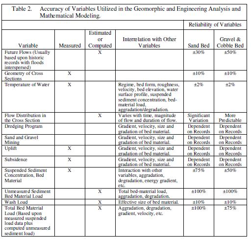
29 accuracy of measured variables that drive the dynamics of the alluvial channel and sediment transport should be understood. For example, it is illustrated in Table 2 that the accuracy of measured variables utilized in the analysis of alluvial rivers may not be as accurate as commonly assumed. For example, measurements of suspended sediment concentrations are collected by depthintegrating techniques over a few seconds. It is not uncommon to encounter variations in collected sediment concentrations on the order of several hundred percent. Likewise, resistance coefficients vary throughout time between wide limits. At lower-regime flow, the Manning s resistance coefficient in a sand-bed channel may be on the order of Conversely, at upper-regime flow conditions, the resistance coefficient may be as low as This means that in an alluvial channel the magnitude of average velocity may vary from 2 to 3 feet per second (fps) to 12 to 15 fps. Also, it will be subsequently proven that in a sand-bed channel, bed-material transport varies on the order of the fifth power of average velocity. Utilizing the velocity extremes above, transport may increase hundreds to even thousands of times. A fundamental concept is that one should not expect the results of an analysis to be acceptable unless the analysis is driven by a database that considers the magnitude and range of variables. It is not acceptable to assign fixed values to these variables in an alluvial channel. 19

30 20

31 21 Figure 10 illustrates the variability in measured concentration of suspended sediment within the sample zone versus flow. This figure is based upon data collected at the Talbert Landing gage on the Mississippi River. Note that the scatter for a specific flow at this station varies on the order of from Cppm = 10 to 200. These easurements of suspended sediment are for the sand fraction size only, i.e., the sampling does not report the concentrations of silt and clay, which are considered wash load, nor do the measurements reflect the bed material moving in the unsampled zone. Figure 10. Ninety-five percent prediction interval for regression of the measured concentration and discharge. 2.6 The Three-Level Analysis of Alluvial Rivers Simons and Li (1982) first proposed the three-level analysis of alluvial rivers. The analysis is composed of three parts: Geomorphic and Environmental Analysis Engineering Analysis Geomorphic, Engineering and Modeling Analysis

32 22 The analysis may be terminated at any level if sufficient conclusions have been reached to make a decision regarding the objectives. The components of the three-level analysis are clearly demonstrated in Table 3. Sediment transport, except in a qualitative way, is not employed in the geomorphic analysis. Lane (1957) proposed one important component of the geomorphic analysis. His concept is expressed as QS Q d50s where Q is the flow of water in cfs, S is the slope of the energy gradient, Qs is bedmaterial transport and d50 is the median diameter of the bed material. It is now known as the stream power equation. Lane s stream power relationship for bed-material transport even preceded the stream power theory presented by Bagnold (1966). The Lane Relationship was modified by Simons in 1975 (Richardson, et al, 1975) to include wash load (C), which may affect the fall diameter of the bed sediment, bed roughness, and bed-material transport to yield d50 QS Qs ( 1) C QSC d Q s ( 2)

33 23

34 24

35 25 3. RESISTANCE TO FLOW IN ALLUVIAL RIVERS One of the major problems of great importance and concern to the analysis of hydraulic conditions in alluvial rivers is the estimate of varying resistance coefficients and velocities, Simons and Richardson, (1963, 1966), Richardson, et al. (1975, 2001), Vanoni (1975), Simons, et al (1999). When considering natural channels and floodplains, including where flow is impeded and ponded by water resources development projects such as dams, reservoirs, bridges, diversions, contractions, and pipeline crossings; utilization of reliable resistance coefficients

36 26 is essential. When analyzing alluvial rivers that are affected by observed and computed geomorphic and hydraulic processes, in the design and/or the evaluation of variables that may affect the design, it is necessary to evaluate these processes both as affected naturally and affected by man s developments. The variables that must be evaluated include the backwater profiles; aggradation; degradation; flood control; groundwater levels; bank stability; bank stabilization; and the design and analysis of bridges, diversion structures, and pipeline crossings. If errors are to be minimized, properly selecting roughness coefficients for alluvial channels and floodplains is a fundamental concern that must be approached by utilizing existing knowledge, field studies, relevant research, and experience with similar systems. In the era of mathematical modeling of river systems, the most important part of modeling is being knowledgeable of the physical characteristics and the properties of the system, including the supply of sediment, as well as the historic dynamics of the reach being investigated, Simons (2000). Hydraulic engineers investigate the sites being modeled to become knowledgeable about the specific physical conditions of the watershed and channel system, both past and present. From this investigation, every practical attempt should be made to estimate accurately the resistance to flow in the specific reach of channel being analyzed. The following is a discussion of an overview of channel classification and selection of roughness coefficients for both channels and floodplains. 3.1 Classification of Open Channels There are numerous different types of open channels. Broadly, they may be classified as: Alluvial channels with mobile boundaries, at least during periods of floods. Rigid channels with significant alluvial deposits on the bed of the channel that may affect resistance coefficients. Rigid-boundary channels that never develop an alluvial bed. Overbank flows that can be characterized by major variations in resistance, over time and distance, depending upon geometry, vegetative state, flow history, and depth of flow. This discussion is limited to meandering, straight, and braided alluvial channels with mobile beds and floodplain inundation. The classification of fluvial rivers can be initially subdivided based upon the physical characteristics of the bed material as follows in Table 4.

37 27 1 Alluvial bars are illustrated in Highways in the River Environment, Richardson, et al. (1975, 1990) and River Engineering for Highway Encroachments, Richardson et al. (2001), Simons and Richardson (1963, 1966), Vanoni (1975), and Simons and Sentürk (1992). 2 Bed forms in sand-bed channels are illustrated in Simons and Sentürk (1977, 1992). 3 Alluvial channels may exhibit strong tendencies to meander at low and modest flows. Conversely, at flood stage they may tend to straighten, even become braided, depending upon energy of the flow, sediment supply, and sediment transport within a specific reach of channel. 4 Resistance to flow may be significantly less than suggested for gravel-cobble and cobble-bed alluvial channels if at flood flow there is a large sand and fine gravel load that can smooth the bed. 3.2 Variation of Manning s Resistance Coefficient for Alluvial Channels Alluvial channels may exhibit significantly differing resistance to flow considering the range of flow conditions and the variety of rivers operating under varying geomorphic conditions and subjected to changes due to developing water resources programs. In order to ascertain responses of alluvial systems, the most important variable is velocity and the Manning s Equation is utilized to determine velocity, if it is not measured. The Manning's Equation in English Units is the following: n 2 / 3 1/ 2 U R S (3)

38 28 where u is the average velocity feet per second in the natural channel; R is the hydraulic radius in feet; S is the slope of the energy gradient, and n is a measure of resistance to flow for open channels. The general approach proposed by Arcement and Schneider (1989) for estimating resistance to flow in a river is defined in the following equation: n nb n n n n ) m ( 4) ( where nb is the base value for a straight, uniform channel; n1 is the value for surface irregularities in the cross section; n2 is the value for variations in shape and size of the channel; n3 is the value for obstructions; n4 is the value for vegetation and flow conditions; and m is the correction factor for sinuosity of the channel. Arcement and Schneider also suggest that the n-value describing resistance to flow on floodplains be as follows: n nb n1 n3 n4 (5) (5) where nb is the base value of n for a bare-soil surface; n1 is the value to correct for surface irregularities; n3 is the value for obstructions; and n4 is the value for vegetation. Table 5 indicates the adjustment factors for the determination of n values.

39 29 The hydraulic radius and slope of energy gradient are precisely defined but may not always be precisely determined. However, error in determining R and S can be minimized by careful field measurements and adequate knowledge of river response to varying flows. What about resistance to flow? Resistance to flow can vary significantly with type of alluvial channel, regime of flow, gradient, geometry of channel, flow, form of bed roughness, grain roughness, width/depth ratios, bank alignment, vegetation, and operation of the system which may impose rule curves where hydropower and flood control requirements are imposed. The bed configuration in alluvial channels is a function of the interaction of the flow and the bed material. As Simons and Richardson (1963, 1966) point out

40 30 in sand channels, the bed form may be bed ripples, dunes, plane bed, standing waves or antidunes depending on the bed-material size, shear stress or velocity, water temperature (viscosity) and concentration of silts and clay. Based on resistance to flow and sediment transport, Simons and Richardson separated the bed forms into a lower-flow regime and upper-flow regime with a transition between the two. The lower-flow regime has ripple or dune bed configuration with large resistance to flow and low bed-material transport. The upperflow regime has plane bed, standing waves or antidunes with low resistance to flow and large bed-material transport. The transition has bed configurations of washed-out dunes. The bed forms and flow regimes are illustrated in Fig. 1. For coarser bed material alluvial channels (gravel, cobbles or boulders) the bed configuration may be dunes, bars, plane bed or antidunes. One of the conditions in the definition of an alluvial channel is that at some discharge the bed material is moved by the flow. With sand-bed material, the bed material moves at all discharges. With the coarser-bed materials, the bed material will move only at larger discharges. The general range of Manning's resistance coefficient for lower and upper regime is presented in Table 6 for each type of bed material identified in Table 4. Note that (1) Within lower regime with silt and sand beds, with sand beds, and with sand and gravel bed, bed forms such as dunes are important variables affecting Manning s n, and n is relatively large. (2) With an overload of sand and silt, coarse bed-material channels may exhibit values similar to sand-bed channels and may experience upper regime conditions. (3) Within upper regime conditions with silt and sand beds, with sand beds, and with sand and gravel beds; the above bed forms give way through a transition zone to plain or flat bed, standing waves, and antidunes with increasing velocity and shear

41 31 stress. With upper regime flow conditions, Manning's n is relatively small resulting in higher velocities, smaller hydraulic radius, increased bed-material transport, and significantly increased channel dynamics. (4) Considering stage discharge relations for alluvial channels, there is often considerable scatter around the mean. This scatter should not always be interpreted as measurement error. Most observed deviations from the mean are not errors in observations and measurements, but due to varying roughness coefficients. In fact, two enveloping curves should be fit to the stage discharge data defining the stage discharge relationship, see river stage vs. discharge in Table 1. The upper curve should be utilized for design of levee height and for evaluation of backwater. The lower curve should be used to compute average velocity through the continuity equation to evaluate channel stability, bedmaterial transport, and stable channel design. This procedure will insure conservative design for both purposes. Also, analysis of change in stage-discharge relations and the use of specific stage relations may indicate stability, aggradation, or degradation. 3.3 Form Roughness The bed forms in an alluvial channel are as varied as the total spectrum of bed forms experienced within both lower-regime and upper-regime flow conditions as one considers the width of the alluvial channel in flood stage. That is, it is not uncommon to find a flat bed with a smooth water surface or standing waves in the thalweg of the alluvial channel and an array of ripples and dunes in regions of the streambed where the energy supports only lower-regime flow conditions. Other pertinent observations, based upon research and experience, verify that: (1) Ripples do not form if the median diameter of the bed material is coarser than about 0.65 mm. (2) Bed material coarser than 0.65 mm but mobilized by the velocity required to initiate general movement of bed material, has the capability to form dunes and bars. (3) With very coarse bed material, the flow may not be capable of mobilizing general transport of bed material except for large floods. Additionally, there may be tributary bars, and, in particular in alluvial channels that experience a significant reduction in slope, the formation of alluvial fans, National Academy Press (1996). Also, when flow encounters major obstructions, both natural and man-made deltas are formed. For example, the Mississippi River delta is created as flows in the Mississippi River encounter the Gulf of Mexico, and deltaic deposits form when flowing water and sediment encounter ponded water formed by a dam or other obstruction. Man's efforts to develop property on riparian land adjacent to alluvial fans and those lands

42 32 upstream of deltas, commonly referred to as estuaries, are particularly challenging if developments such as bridges, diversion structures, navigation channels, etc. are constructed. 3.4 Selecting Roughness Coefficients for a Practical Case To demonstrate the importance of properly selecting roughness coefficients, consider the construction of a major dam on an alluvial river. The problem of interest is the determination of the amount of backwater that causes deposits of sediment in the backwater-affected reach. The dam forms a reservoir that provides limited flood control and is operated to generate hydropower. The release of stored floodwater may be ordered to optimize hydropower and navigation both upstream and downstream of the dam, and to limit flooding of riparian lands upstream of the dam. The recognized impact of the dam, its reservoir, and its rule curves (governing the release of water) is generation of backwater. Backwater is the difference between the elevation of the water surface profiles before building the dam and after building the dam. Historically and presently, backwater effects are calculated utilizing widely accepted one-dimensional mathematical models such as HEC-2, HEC-RAS, GSTARS 2.0, HEC-2QS, and UNET. The UNET models are more acceptable than HEC-2 and HEC-RAS where rivers are relatively flat and they encounter relatively large impoundments where the peak flow and peak stage may become uncoupled. The data required for determination of backwater include: cross sections of the channel extended over adjacent floodplains; hydrologic conditions to be evaluated; and the selection of Manning's Roughness Coefficient if Manning's Equation is utilized in the analysis, see Eqs. (4) and (5). The accuracy with which pertinent variables can be calculated or estimated is of paramount importance to the accuracy of backwater calculations. Manning's n is a measure of resistance to flow in unimpeded natural channels. Manning's n for this condition varies with regime of flow, the geometry of the system, bank stability, and the presence of bank line vegetation. In addition, n values must be determined or estimated for the floodplains adjacent to the channel if an accurate determination of backwater effects is to be achieved. Because of the large number of factors affecting roughness in a natural channel, it is essential in the estimate of n to be knowledgeable regarding open channel flow as observed in alluvial systems. To determine the Manning s n, it is necessary to review recent relevant research regarding resistance to flow in alluvial channels. One should compare field observations with similar river systems that have been accurately analyzed and field studies within the reach in

43 33 question that permit back calculation of the Manning's n value from the Manning Equation. 3.5 Data Required to Estimate Manning's n, Velocity, Stage, and Sediment Transport In the river environment, it is generally accepted that resistance to flow in the alluvial channel is much less than the resistance encountered by the flow on the floodplain. This is generally correct Data Required for Alluvial Channels A. Maps 1. USGS quad sheets. 2. Other pertinent topographic maps that may exist. B. Aerial photographs taken over time. C. Flows 1. At gaging stations, if available. 2. If flows are not available, collect precipitation records and simulate floods. Also compare with similar systems where data are available. D. Sediment discharge data, if available. Aggradation and/or degradation in the backwater environment can significantly increase backwater caused by impoundments with time. E. Conduct a flow frequency study to establish Q5, Q10, Q25, Q50, Q100, Q200, and Q500 F. Estimate channel stability: i.e., note sloughing banks, bank's alignment, presence of snags, presence of bank vegetation, and presence of bars. G. Collect and analyze samples of bed material to determine which type of bed material of the alluvial channel is relevant, i.e., sand, gravel, etc. H. Access FEMA studies and/or comparable (FEMA flood studies are to establish flood insurance rates only) for: channel cross sections, floodplain cross sections, Manning's n values adopted by FEMA, flow frequencies, geometry and location of bridges, contractions, etc. I. Make field estimates of Manning's n for existing flow conditions. J. Note the turbulence of the water surface and obvious hydraulic conditions, in particular: boils on the surface that may verify the existence, spacing and height of dunes; test to evaluate whether subcritical or supercritical flow conditions exist; quantify floating debris; note how hydraulic conditions may change with stage and discharge; and determine the location of a thalweg.

44 34 An appraisal of collected data will assist in the selection of an acceptable Manning's n value. More specifically at this point in the analysis, the following knowledge should be available. A. Type of river: meandering or braided. B. Range of flows: small, medium, large. C. Type of bed material: sand, gravel, etc. D. Conditions related to bank roughness. E. An estimate of Manning's n values for existing field conditions - this is very important. This can be accomplished by collecting field data for the river in question for a range of flows. Such an approach requires collection of field data so that the Manning's resistance coefficient can be calculated and evaluated based upon conditions at which pertinent field data were collected. Cross-sectional data to be evaluated including: Wetted perimeter (p), Cross-sectional area (A), Hydraulic radius (R = A/p), Discharge flow (Q), Mean flow velocity (u = Q/A), Longitudinal profile for channel slope (S) Data Required for the Floodplain A. Gradient of the floodplain. B. Topography of the floodplain. C. Width of the floodplain - wide floodplains signal flat channel slopes. D. Land uses on the floodplain. E. Types of obstructions on the floodplain - farming, pastures, trees, fences (orientation - density and trapping of debris), cross roads, fences and vegetative hedges and cross drainage, buildings, dikes, etc. F. Photographs of the river and floodplains during flooding. G. Note the velocities on the floodplain and observe flow at obstacles like approaches to bridges; also look for overtopping of bridges oriented transverse to the flow. On most floodplains, the resistance to flow, the number of obstructions and the minimal slope of wide floodplains dictates that ponding on the floodplain, not flow on the floodplain, is common. However, in considering alluvial rivers with wide floodplains, subchannels may develop from the outside of one bend to the inside of the next bend downstream because this is the path of maximum energy gradient. 3.6 Concepts to Remember The common tendency is to overestimate the resistance to flow in alluvial channels and underestimate the resistance to flow on the floodplain. These

45 35 erroneous assumptions have significant effects on velocity, river stage, regime of flow, and bedmaterial transport. 1. Resistance coefficients - generally the Manning n values - are highly variable over time and distance, and generally are much more difficult to estimate accurately than most engineers realize, especially in openchannel, alluvial flow cases, and in floodplain flow situations. Inaccuracies of up to one order of magnitude are not uncommon when estimating n on the basis of inadequate experience and no field data. No other variable in hydraulic equations and mathematical models is more elusive or more important. Rate of discharge, stage of flow, and average velocity the common unknowns are more sensitive to selected n values than to other variables. 2. Assignment of incorrect n values for channel and overbank areas as inputs to mathematical models is common. Typical values are selected using textbook tables, photographs, and possibly a brief site visit. Selection of n values when done lightly, hurriedly, or without due regard for the intricacies and factors involved, can have enormous adverse consequences. 3. There is no single, specific n value for a given reach of an alluvial stream that experiences different flows. There are numerous n values, each dependent upon a number of imposed, interdependent variables. A list of only a few obvious ones would include: grain sizes of bed material, bed forms, discharge, velocity, depth of flow, suspended and bed sediment loads, plan form of the river, state of vegetation, cutoffs, bank stabilization, dredging, ice jams, log jams, etc. To this list we should add: historical and recent discharge that affects bed profile and bed forms; major obstacles and conditions in channel and, especially, in overbanks, which may cause general loss of conveyance and create specific sites of nonconveyance or redirection of flow; backwater conditions which take flow out of uniform, normal flow regimes; duration of flood; and others. 4. Resistance coefficients are usually considered to be a representation of friction, but many flows of interest, including 100-year floods, may be influenced more by form loss than by grain resistance. When moving from the laboratory, through the moderately large, natural river flow, up to flood flows, including overbank flows, the concept of n as a resistance coefficient alone must be replaced by a combination of resistance and form losses, see Eq. 4 and Table 5. In many instances, it is incorrect to assume the same Manning s n for the 100-year flood

46 36 and average flow conditions because of changes in bedforms and gradient. 5. One should be aware of the "overbank paradox: When floods cause streams to rise and flow above the channel out into overbank areas, direction of flow can abandon the channel's thalweg and bankconstrained pattern, which is often a meandering one, in favor of a more straight, down-valley orientation. This will change the gradient drastically. On the other hand, when very wide floodplains are flooded, there is often a very high resistive condition on the overbanks, caused by forests, downed timber, fences, road and railroad embankments, and structures. Such conditions can convert the overbank "flow" area to a series of ponds, or ineffective flow areas. Failure to distinguish between these two counterinfluencing conditions, and to properly simulate them through proper n values or other modeling adjustments, can result in erroneous and misleading results. 6. The thalweg straightens as flow increases in meandering channels causing as much as 10 to 20 percent increase in slope. 4. BEGINNING OF MOTION 4.1 Introduction The shear stress at which a given size of sediment particle begins to move is important. When the drag force is less than some critical value, the bed material of a channel remains motionless. Then the alluvial bed can be considered as immobile. But when the shear stress over the bed attains or exceeds its critical value, particle motion begins. In general, the observation of particle movement is difficult in nature. The most dependable data available have resulted from laboratory experiments. The beginning of motion is difficult to define. This difficulty is a consequence of a phenomenon that is random in time and space. When the shear stress is near its critical value, it is possible to observe a few particles moving on the channel bottom. The time history of the movement of a particle involves long rest periods. In fact, it is difficult to conclude that particle motion has begun. Kramer (1935) and Buffington (1999) proposed four levels of motion of bed material. 1. None.

47 37 2. Weak movement: Only a few particles are in motion on the bed. The grains "moving on one square centimeter of the bed can be counted." 3. Medium movement: The grains of mean diameter begin to move. The motion is not local in character but the bed continues to be plane. 4. General movement: All the mixture is in motion; "the movement is occurring in all parts of the bed at all times." Whether or not a plane bed can exist with weak to medium sediment motion is debated; though positive evidence of its existence has been presented by Liu (1957) and others (Sentürk, 1969). However, Liu s observations may have involved shallow flow where the Froude number was equal to or greater than 1, F u / gd 1 r. This hydraulic condition would dictate that the plane bed occurred in upper regime. But the complexity of the phenomenon is generally accepted. In fact, many researchers such as Schoklitch (1914), Kramer (1935), Shields (1936), White (1940), Tison (1953), Simons and Richardson (1966), Vanoni (1964) have attempted to solve the problem of initiation of motion. Still the exact solution continues to defy precise analysis. The complexity of the problem explains the diversity of experimental results. In reality, there is no truly critical condition for initiation of motion for which motion begins suddenly as the condition is reached, or if it exists, it is undefinable. Data available on critical shear stress are based on more or less arbitrary definitions of critical conditions. Most definitions used have relied on direct visual observations, which turn out to be subjective. There is no evidence that the mean diameter represents most correctly the composition of a mixture. The engineer facing this dilemma of dealing with a mixture of sediment sizes should analyze his problem very carefully, and then select a formula that best suits the physical conditions. 4.2 Representative Diameter of a Bed-Material Mixture The determination of the size of a particle that represents a sediment mixture is difficult. There are no fixed criteria to apply. For this reason, different particle sizes have been proposed as representative including the d35, d50, dm, -- d100 sizes. Figure 11 can be used to determine the representative grain size of a sand or gravel mixture (Simons and Sentürk, 1992). Collecting and analyzing representative samples of bed material permits the evaluation of the mixtures. 1. The mixture is separated into size fractions by mechanical analysis. 2. A diagram similar to Fig. 11 is prepared. 3. The size distribution of the mixture is determined experimentally and utilized, as illustrated on Fig. 11.

48 38 In studies of scour below culvert outlets in alluvial channels, Stevens (1968) was able to consolidate a wide range of scour data by employing the expression /3 i1 k ( 6) for the effective or representative grain size of well-graded materials. Here d 1) 0 d i (7) 2 10 d i ( d 2) 10 d i 2 20 d i ( d 10) 90 d i d i (

49 39 Figure 11. Size frequency distribution curve showing dm, d35, d50, d65, d85 and d90 (Simons & Sentürk, 1992). The terms d0, d10,, d100, are the sieve diameters of the bed material for which 0 percent, 10 percent,, 100 percent of the material (by weight) is finer. Stevens equation is the equivalent to utilizing the arithmetic average of the sum of the weights of the individual particles.

50 Theoretical Considerations Water flowing over a bed of sediment exerts forces on the grains. These forces tend to move or entrain the particles. The forces that resist the entraining action of the flowing water differ depending upon the properties of bed material. For coarse sediments such as sand and gravel, the resisting forces mainly relate to the weight of the particles but also are a function of size and shape of particle, its position relative to other particles, and form of bed roughness. When the hydrodynamic forces acting on a grain of sediment have reached a value that, if increased even slightly the grain will move, critical or threshold conditions are said to have been reached. Under critical conditions, the hydrodynamic forces acting upon a grain are just balanced by the resisting force of the particle. 4.4 Theory of Beginning of Motion are: The forces acting on an individual particle on the bed of an alluvial channel 1. The body force Fg due to the gravitational field. 2. The external forces Fn acting at the points of contact between the grain and its neighboring grains, and 3. The fluid force Ff (lift and drag) acting on the surface of the grain. The fluid force varies with the velocity field and with the properties of the fluid. As both the form drag and viscous shear are proportional to the shear velocity, the ratio of the forces tending to move the grain to the forces resisting movement is F F D v 2 ds u (8) ( ) ) d s gds ( s s Recall that 2 /* o u. The relation between o S s / d and /* d u s for the condition of incipient motion has been determined experimentally by Shields and others. The relation is given in Fig. 12. At conditions of incipient motion, the shear stress o is designated the critical shear stress c.

51 41 Criteria based on velocity rather than shear stress have also been proposed. The values of maximum permissible velocity recommended by Fortier and Scobey (1926) are given in Table 7 for clear flows in channels and water transporting colloidal silts. The Shields parameter has been studied more or less continuously since Rouse (1939a and b) added a defining curve that establishes the constant value of Shields parameter beyond approximately R* = 100. This value of R* is usually exceeded in alluvial rivers. There is generally agreement that the Shields parameter is equal to except for Gessler (1971) whose studies established a value of Shields parameter of Gary Parker (1982) states It thus becomes apparent that neither the value * c of the Meyer-Peter and Müller relation, nor the value * 0.06 c of the Shields diagram provides a very good estimate of critical conditions for the breaking of gravel pavement, regardless of whether pavement of subpavement D50 is used. The Neill (1968) criterion based on pavement is preferred. Note that pavement means armor. Gary Parker utilizes a Shields coefficient based upon Neill s work of Hence we conclude that most studies of Shields parameter have been based on a uniform, nonvarying size and gradation of bed material. In fact we conclude that the value of Shields parameter varies with the physical conditions in the river. That is, whether it is aggrading, degrading, an alluvial fan environment, or it is armored to some degree. Under these conditions it is very difficult to establish a size of bed material and variation of that size with time in the natural environment.

52 42 Figure 12. Shields Diagram: dimensionless critical shear stress. 4.5 Experimental Approaches Beginning of motion of bed material is a function of the dimensionless number o s s / d. A fully developed, turbulent-flow condition was assumed in the derivation of this expression. When viscous effects are not negligible, viscous forces should be considered. The equation for equilibrium of a particle in simplified form is u d s. 2 c. s u cds f v This equation considers viscous effects. Next, consider the evaluation of factors affecting the equilibrium condition of particles when c, the critical shear stress, is defined as 2 c u. c (9) (10)

53 43 and c u* is the critical shear velocity. The turbulent shear velocity ' ' u. u v (11) is derived from turbulence theory. When the flow is laminar u* = 0 (neglecting purely viscous shear). When the flow is turbulent, the Prandtl-von Kármán semilogarithmic velocity equation can be used to obtain o. The resulting relation shows that u1 u2 u. (12) 5.75log( y / y ) 1 2 where u. = /. 0

54 44 When computing u* from Eq. 12, the velocities should be measured near the bed because these values are directly involved in the initiation of motion. Note that u* is assumed to be constant in the derivation of Eq. 12. It is this assumption that allows engineers to compute u* from the relation If velocity profiles are not known, the relation u. grs (13) RS 0 (14) may be used to estimate an average value of o for the channel cross section if the channel is uniform. Research conducted on the initiation of particle motion has almost exclusively utilized nearly uniform material. For application of these results to the motion of nonuniform granular material, the median grain size is suggested. Various efforts have been directed towards the analysis of the behavior of granular mixtures. Egiazarof (1965) proposed the following equation for incipient motion for a mixture of nonuniform particles c ( ) d s d log19 d 50 s 2 (15) where 50 d and s d are the median and the average diameter of grains, respectively. With a fine-graded mixture s d d 50, the resistance to incipient motion is increased, while according to Eq. 15 the opposite is true for a coarsegraded mixture where s d d Shields Diagram Many experiments have been conducted to develop an explicit solution of Eq. 9. The earliest one is the graphical presentation given by Shields1 (1936). The Shields Diagram (Fig. 12) is widely accepted and c s s /()d is often referred to as Shields parameter. Shields determined this relationship by measuring bed-load transport for various values of s s /()d at least twice as large as the critical value and then extrapolated to the point of vanishing bed load. This indirect procedure was used to avoid the implications of the random orientation of grains and variations

55 45 in local flow conditions that may result in grain movement even when s s /()d is considerably below the critical value. The Shields Diagram can be divided into three regions as illustrated in the following. Region 1:2 / 3.63 ~ 5.0 In this region 3s d, where * 11.6/ u, and the boundary is considered hydraulically smooth (is the thickness of the laminar boundary layer). Shields estimated the portion of the diagram for / 2 * s u d. He did not perform any experiments in that region.3 According to Shields, when the value of c 0.1 ( d then (approximately) s s u. d v Region 2: 3.63 ~ 5.0 / 68.0 ~ 70.0 s 100 (16) In this region, the boundary is in a transitional state and / 3 6s d. For this region, k 1 ksu 11.6 v s. (17) The Shields Diagram has a form similar to Darcy-Weisbach's resistance coefficient f versus Reynolds number Re. Also, it is similar in form to the relation between the drag coefficient Cd and the Reynolds number Re for cylindrical bodies and to the relation between v / * s uk and ( /v* s B f u k ) proposed by Nikuradse (1933). The minimum value of c S s F /( )d * is ~ and the corresponding value of v/ * * s R u d is about 10.4 If s d is computed from these values of * R and * F, it can be seen that d m mm ft s For larger diameter particles, ripples do not form; dunes form on the bed. 5 Region 3: / 70 ~ 500

56 46 In this region, the boundary is completely rough and * F is independent of Reynolds number * R and is equal to u ( ) d s s (18) The upper limit of * R in Region 3 is subject to discussion. Some researchers have given values as high as 1,000 for * R. Considering * F, Meyer- Peter and Müller (1948) suggest a value of instead of 0.06, but 0.06 is most generally accepted. However, it is suggested by Simons (Simons and Sentürk (1992)) that by collecting data on initiation of particle motion under field conditions permits selection of a more precise value for the particular channel. However, observing or identifying initiation of particle sizes by utilizing observed values or by trapping particles in motion over a range of discharges is extremely difficult. It must be done with considerable care and with knowledge of channel geometry and hydraulic conditions at the cross section and upstream of the selected cross section. This is particularly true for gravel- and cobble-bed streams. 4.7 Other Formulae Defining the Beginning of Motion Over the past 50 years, numerous papers have been published defining the beginning of motion, most of them more or less intensive variations of the original Shields' work (for example, Ippen and Verma, 1953; and Bogárdi, 1965). These papers seemed to originate from the fact that the Shields Diagram is somewhat unhandy to apply because the dependent variables (critical shear stress or grain size, depending on the problem) appear in both ordinate and abscissa parameters. A solution of the Shields Diagram, Fig. 12, presented by the "Task Committee on Preparation of Sedimentation Manual" (1966) utilizes a third parameter ds v s 0.1 1gd s (19) Entering the diagram and following the correct parallel line, one can determine its intersection with the main Shields curve and the corresponding value of * F. Sentürk (1969), using a diagram given by Simons and Richardson (1961), has prepared a diagram for solving engineering problems that avoids trial and error. When the fall velocity and the size of grains are given, it is possible to obtain

57 47 directly the corresponding value of / *u d. The fall velocity can be determined from Fig. 13 (from Fig. 2 in U.S. Inter- Agency Report No. 12, 1957). Natural sediment has a shape factor of about The shape factor is c / ab where a, b and c are mutually perpendicular axes of the particle of sediment and c is the shortest dimension, b is the intermediate dimension, and a is the longest dimension of the particle, Albertson (1952) and Shultz, et al. (1954). Figure 13. Relation of nominal diameter and fall velocity for naturally worn quartz particles with shape factors (s.f.) of 0.5, 0.7, and 0.9 (from Inter-Agency Report No. 12, 1957). 4.8 Application of Beginning of Motion to Practical Problems Many sediment transport equations can be expressed in the form Q ) n s K( o i (20) where: is the bed-shear stress; K o o is the shear stress for incipient motion for a given particle size; is a coefficient that ranges with sediment size, channel dimensions and

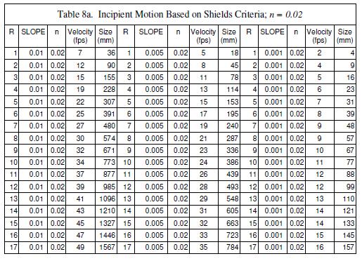
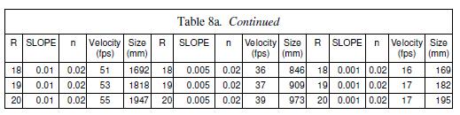
58 48 n gradient, etc.; and n is an exponent that varies with sediment size, channel dimensions, flow, channel gradient, etc. Similarly, an expression for critical velocity, critical slope, etc. can be derived for a given set of conditions. An example of application of Shields Criteria for beginning of motion is illustrated in Fig. 14. Such relationships for any alluvial channel can be formulated from Tables 8a and 8b. This table was developed for n values of 0.02, 0.03 and 0.04 for channel slopes of 0.01, 0.001, and for a range of depths of 1.0 to 20.0 feet. Figure 14. Incipient motion based on Shields Criteria n = 0.04.

59 49

60 50 Example Problem Regarding Application of Shields Relationship to Armoring Problem The Gila River flows southwest, south of Phoenix, Arizona. The plan form of the Gila River is braided during flood flows. During minor flows contributed by sewage treatment plants upstream, the low-flow channel tends to meander on the bed occupied by larger floods, Lane (1957). Consider the potential degradation for the 100-year flood near the bridge crossing the Gila River on State Highway 85. For determination of this flood, it is required to analyze existing hydrologic data or synthesize the 100-year flood event. The calculation of potential degradation may be accomplished in two ways: (1) application of Shields Criteria or (2) routing of water and sediment by size fractions utilizing some proven mathematical model. Considering the Shields approach, certain field data and hydrologic data must be determined. An analysis of sediment sizes comprising the bed of the Gila River and its floodplains must be conducted in depth to determine the gradation of the natural material and the potential for development of an armor layer. The characteristics of the floodplain and bed sediment are illustrated in Fig. A.

61 51 Figure A. Bed material and armor layer, Gila River. Figure B. Gila River 100-year hydrograph at State Highway 85. Solution Proceeding with the Shields analysis using F*=0.047, the basic Shields equation is

62 ( ) d (21) c s s The critical velocity equation using the Weisbach f for fully developed turbulent flow is 1/ 2 8 c uc (22) f Solving these two equations for uc with f=0.0495yields 1/ 2 uc 20.1d s The plot of this equation is illustrated on Fig. C. Figure C. Critical size of bed material related to velocity in the Gila River channel. Then complete a hydraulic analysis for the peak flow. This may be completed for the sections involved or it would be preferable to run a mathematical program, HEC-2 or HEC-RAS, to determine the average velocity. Utilizing the selected method, the average velocity was determined to be 8.2 fps. And referring to Fig. C, it is determined that the maximum size of sediment transported by the flow da is 50 mm. The equation for maximum degradation to form an armor layer is

63 53 and ZP 2 c d a 2d Z P In this equation, Pc is the percent of sediment coarser than 50 mm. Referring to Fig. A, it is observed that 3 to 5 percent of the sediment is coarser than 50 mm. Hence, A varies from 7 to 11 feet. An investigation was conducted for evidence of past armoring and evidence was found that armoring of the bed had occurred in past floods. A typical patch of exposed armored bed is shown in Photo 1. A pebble count of the exposed armor was conducted, and it yielded a percent finer curve as shown on Fig. A. The armor layer was observed at an elevation about 12 feet below the floodplain. From the size of the particles forming the armor layer and from the elevation of the armor layer, it was determined that this armor coat was formed by a flood exceeding the peak discharge illustrated in the 100 year flood hydrograph. c a Photo 1. Typical patch of exposed armored bed in Gila River, Arizona, near State Highway 85 Bridge, May, 2001.

64 54 5. SEDIMENT TRANSPORT 5.1 Historic Note The quest for a universal bed-material transport equation has been a goal of the engineering profession for several centuries, probably starting in China with similar quests for a suitable equation applicable to sediment transport in alluvial rivers throughout Europe and Asia. The search has continued and universities and governmental agencies throughout the world have made continuous attempts in recent decades. Some of the most notable equations for bed-material transport in alluvial channels are listed in Table 11 on Page 61 of this paper. These equations, when used under the conditions that were adopted in their development, give acceptable results. This is surprising considering the natural variability in bed-material transport and the broad range in the quantity of sediment transported at any discharge. Transport, as computed by these equations, in general displays an error on the order of 100 percent for field conditions, for example, see Fig. 21. The most reliable method is the modified Einstein method (Colby and Hembree, 1955; Colby and Hubbell, 1962). With extensive sampling results, most equations can be made to work very well. The reason is that most of the suspended bed-material discharge is measured within the sampled zone and the measurements are used to compute the bedmaterial discharge in the unsampled zone. The modified Einstein method can be used to calibrate the other equations or validate their results. Also, the method can be used along with measured suspended sediment records at a given site to determine the coefficients in the following equation: where b Qs aq (23) Q s = sediment discharge (bed material or total )Tons/day; Metric tons/day Q = water discharge, cfs, cms a &b = coefficients determined from measured data The field measurements required to utilize the modified Einstein includes the wash load. That is an additional advantage of using this method. In using these equations and in making sediment discharge measurements, the following enumerated concepts must be observed.

65 55 Suspended sediment samples using depth-integrating sampling techniques are only a snap shot of the suspended sediment concentration of the sediment discharge passing a cross section at a given time. Considering the variation in concentration and sediment discharge at a cross section with time (Figs. 17 and 18), t requires many samples and a long-time sediment discharge record to obtain an accurate sediment discharge. This record could be the average sediment discharge in tons per year or a sediment discharge-rating curve of sediment discharge as a function of the water discharge, etc. Most sediment transport relationships are heavily dependent upon flume data and limited stream data. This causes some distortion in dimensionless parameters because: Varying the slope has increased the range of dimensionless parameters from flumes. The range of dimensionless parameters experienced in rivers is primarily from variation in discharge. Most river data include suspended bed-material discharge (load) only and must be corrected for the unmeasured bed-material discharge. Most relationships were developed for a limited range of grain sizes comprising the bed material. Transport equations tend to over-predict sediment transport because lack of recognition of the influence of gradation of bed material on bed-material transport. Hydraulic and transport conditions vary widely from channel system to channel system; too wide a range of conditions to be covered by one transport equation. For example, variations result from size of rivers, range in sizes and gradation of bed material, subcritical and supercritical flow, lower-regime and upper-regime flow, bed forms including bars, sediment supply, aggradation and degradation, armoring, expansion and contraction of the bed material related to regime of flow, etc. It is difficult, if not impossible, to measure total sediment transport for the total range of flows in alluvial channels. The modified Einstein method can, however, overcome this difficulty. Suspended samples of transported sediment are collected within the sampled zone only. Calculations may be made of the bed-

66 56 material transport in the unsampled zone but they are costly and many calculations are required. More recently, there has been an attempt to utilize bed-load samplers to quantify this missing data, see Sec Simons and Richardson collected samples of total bed-material transport using the 8-foot, 200-foot long recirculating flume at Colorado State University. They collected 80-pound samples of water and sediment discharged from the flume every five minutes. The maximum difference between sample concentrations was 1200 percent with an average of 80-pound samples collected over two hours; the average concentration was judged to be within 5 percent of the true average concentration of bed-material transport. Similar conditions, but much more adverse to an accurate collection procedure, occurs in the field. For example, refer to Fig. 10 that illustrates average concentrations resulting from the sampling procedure at a cross section in the Mississippi River. Normally two samples are taken in each vertical in shallow streams. With the ETR method, sampling takes from 10 minutes to an hour or more depending on stream size. Samples are only a snapshot of the suspended sediment considering long-time average suspended sediment concentrations and bed form. The sediment transported in contact with the bed (bed load) is very difficult to measure. In most sampling environments, it is missing. This means that in shallow, high-velocity alluvial channels, the measured suspended load may only range from 50 to 80 percent of the total sediment discharge. The unmeasured bed load is on the order of 50 percent of the total load and it, for the most part, has not been sampled. It can be concluded that measured sediment concentrations may not measure the average concentration at any given time. At present, when bed load is measured, the adopted procedure is to utilize the Helley-Smith Sampler. However, this sampler is not utilized in standard sampling procedures. It may be impossible, or at least foolhardy, to sample alluvial channels when they are at flood stage, except from a bridge if it is still standing. Very sparse data are available during floods in alluvial channels. To emphasize the problem, it is during floods when the bulk of the bed material is transported and major

67 57 channel changes are occurring. It has been concluded theoretically and by limited sampling that in sand-bed channels the transport of bed material varies as the 5th power of average velocity. In graveland cobble-bed channels, the transport of bed material varies as the 3rd or 4th power of average velocity. The role of fine sediments, generally classified as wash load, is poorly appreciated. Haushild, et al (1961) verified that the presence of a significant concentration of clay and silt in the flow reduces the fall velocity of bed material, particularly with bentonitic clays and sand-bed channels, see Figure 15a that resulted from Haushild, Simons, and Richardson s research at Colorado State University. Also, the effect of temperature of water on fall velocity of bed material is illustrated in Figure 15b. Figure 15. Variation of fall velocity with temperature and concentration of fine sediment. Most research applied to bed-material transport in alluvial channels has ignored the size of channels and the range of bedmaterial sizes in their research. Only a few equations have resulted from research that recognizes gravel and cobble gradations of bed material, notably equations introduced by Meyer-Peter, Müller, Yang, Shen, Simons, etc. (Simons & Sentürk, 1992). It is extremely difficult to determine the size and gradation of bed material, particularly in channels that involve sand, gravel,

68 58 cobbles, etc. The probable error in such sampling may be on the order of 50 to 100 percent. The problem is further complicated in perennial channels where some sampling must be conducted under water and in the flow. Episodic events have a significant effect on channel geometry and bed-material transport. These events include catastrophic floods, fires denuding watersheds, earthquakes, floods caused by glacial lake outburst floods, failure of dams large and small, etc. In many cases, new channel geometry results from an episodic event. These events are difficult to predict and quantify. The role of man s development of water resources and particularly those affecting hydrology, hydraulics, and sediment supply also has a significant effect on channel geometry and sediment transport. Often man s role has been ignored or inadequately assessed. The routing of water and sediment by one-, two- or threedimensional models is plagued by inadequate appreciation of the limitations of sediment transport relations, inaccurately assessing sediment supply, and often inaccuracy of plan form and profile of the channel and direction of flow. A further problem is orienting cross sections of channels and of floodplains to properly reflect the direction of flow during major floods. In general, major floods occur down valley ignoring bends and meanders in channels filling the existing channel with sediment where the flood channel cuts across existing meanders. In water modeling, as accepted by FEMA, the results are not suitable for engineering analysis and design for the following reasons: 1) The description of the channel and the floodplain may not be current. Those measurements describing the geometry of the system may well be inaccurate, particularly in terms of flow alignment. 2) The cross sections used in the modeling effort are not selected normal to the path of flow of major flood events. 3) The flood profiles and extent of floodplain flooding are principally dictated by analyzing the 100-year event. This flood has a 1 percent chance of occurring in any year. There is a much higher probability that a 5-, 10-, 25-, or 50-year flood will occur prior to the 100-year event. Geomorphically and hydraulically it is common knowledge that any flood, no

69 59 4) matter how small, alters the channel plan form, profile, and cross sections invalidating the computations for the 100-year flood unless the 100-year flood is the first to occur after the modeling analysis is completed. The current methods of prediction of flood stages and average velocities are further limited in such models as the HEC-2 and HEC-RAS for the principal reason that they only route water and assume rigid-boundary conditions. 5.2 Fundamentals of Sediment Transport The transport of sediment in rivers depends upon many interrelated variables. There is no single equation that can be applied for all conditions. Simons and Sentürk (1992), Julien and Simons (1986) based on extensive experience in the laboratory and field, presented recommendations to be followed in sediment transport analysis. Major recommendations include: 1. Examine the available transport equations and determine by testing which one is best for a specific river system. 2. Calculate the rates of transport equations using selected relationships and compare the results with field data. 3. Select the relationships that best agree with field observations and if data are available, refine this relationship so that it is site specific. Additionally, development of rivers for very important purposes, such as dams, navigation, etc., field sediment measurements should be conducted so that the chosen sediment transport relation is validated and extended to a wider range of river conditions. Einstein (1964) stated: Every sediment particle which passes a particular cross-section of the stream must satisfy the following two conditions: (1) it must have been eroded somewhere in the watershed above the cross-section; (2) it must be transported by the flow from the place of erosion to the cross-section. Each of these two conditions may limit the sediment rate at the crosssection, depending on the relative magnitude of two controls: th availability of the material in the watershed and the transporting ability of the stream. In most streams the finer part of the load, i.e., the part which the flow can easily carry in large quantities, is limited by its availability in the watershed. This part of the load is designated as washload. The coarser part of the load, i.e., the part that is more difficult to move by flowing water, is limited in its rate by the transporting ability of the flow

70 60 between the source and the section. This part of the load is designated as bed sediment load. This distinction is important because the bed material is transported at the capacity of the stream and as a function of measurable hydraulic variables and channel geometry. If the sediment supply exceeds the transport capacity, aggradation will occur. Conversely, if the supply is less than the capacity to transport, degradation will occur unless inhibited by the development of an armor layer, controls, etc. Sediment particles are transported by rolling or sliding on the bed (bed load or contact load) or by suspension by the turbulence of the stream. Even as there is no sharp demarcation between bed-sediment discharge and wash load there is no sharp line between contact load and suspended sediment load. A particle may move part of the time in contact with the bed and at other times be suspended by the flow. The distinction is important because the two modes of transport follow different laws. The equations for estimating the total bed-material discharge of a stream are based on these laws. A further subdivision of mode of transport of sediment, including a pictorial representation in Fig. 16, of measured load and unmeasured load follows. When a river reaches equilibrium, its transport capacities for water and sediment are in balance with the rates supplied. In fact, most rivers are subject to some kind of control or disturbance, natural or man made that give rise to nonequilibrium conditions. Total sediment load can be divided into three components (Richardson, et al., 1975, 1990, 2001; Julien, 1995): 1. by type of movement 2. by method of measurement ( L L Ls) (24) T b ( L L Lu) (25) T m 3. by source of sediment ( L L L ) bm T w (26) where LT = the total load, Lb = bed load which is defined as the transport of sediment particles that are close to or maintain contact with the bed,

71 61 Ls = suspended load defined as the suspended sediment passing through a stream cross section above the bed layer, Lm = measured sediment, Lu = unmeasured sediment that is the sum of bed load and fraction of suspended load below the lowest sampling elevation, Lw = wash load which is the fine particles not found in the bed material (ds <d10), and originates from available bank and upslope supply, and Lbm = the capacity limited bed-material load. Figure 16. Classification of sediment transport in rivers. 5.3 Suspended Bed Sediment Discharge The suspended bed sediment discharge in lbs per second per unit width of channel, qs, for steady, uniform two-dimensional flow is q e y ucdy (27) s a where u and vary with y and are the time-averaged flow velocity and volumetric concentrations, respectively. The integration is taken over the depth y between the distance "a" above the bed and the surface of the flow "yo. The level "a" is assumed to be 2-grain diameters above the bed layer. Sediment movement below this level is considered as bed load rather than suspended load. The discharge of suspended sediment for the entire stream cross section, QS, is obtained by integrating Eq. 25 over the cross section to give where Q QC s (28) s is the average suspended-sediment concentration by volume. The vertical distribution of both the velocity and the concentration vary with the mean velocity of the flow, bed roughness, and size of bed material. The

72 62 distributions are illustrated in Fig.17. Also v and c are interrelated. That is, the velocity and turbulence at a point is affected by the sediment at the point, and the sediment concentration at the point is affected by the point velocity. Normally this interrelation is neglected or a coefficient applied to compensate for it. Figure 17. Schematic sediment and velocity profiles. To integrate Eq. 25, v and c must be expressed as functions of y. The onedimensional gradient-type diffusion equation is employed to obtain the vertical distribution for c and the logarithm velocity distribution is assumed for v in turbulent flows, Rouse (1937). The resulting equation is where c ca c c a y y y Z a ya a a (29) = the concentration at a distance y from the bed; = the concentration at a point a above the bed; and Z = /u*, the Rouse number, named after the engineer who developed the equation in Note that when depth y becomes zero, the concentration of suspended sediment is undefined. Figure 18 shows a family of curves obtained by plotting Eq. 26 for different values of the Rouse number Z. It is seen that for small values of Z, the sediment distribution is nearly uniform. For large Z values, little sediment is found near the water surface. The value of Z is small for large shear velocities u* or small fall velocities. Thus, for small particles or for extremely turbulent flows, the concentration profiles are uniform.

73 63 The values of and have been investigated. For fine particles ~ 1. Also, it is well known that in clear water = 0.4 but apparently decreases with increasing sediment concentration. Using the logarithmic velocity distribution for steady uniform flow and Eq. 26 the equation for suspended sediment transport becomes Z y a ya y Xy a qs u. ca a 2.5In dy ya a y k (30) s Many investigators have integrated this equation. Figure 18. Graph of suspended sediment distribution. As shown in Fig. 19, the supply limit range is accompanied by degradation and the capacity limit is accompanied by aggradation. Einstein (1950) defined the wash load as the grain diameter 10 d for which 10 percent of the total bed sediment is finer. Fine sediment load by definition is the load of silts and clays,

74 64 which have diameters smaller than mm. Many engineers assume that the smallest size of bed-material load is equal to or greater than mm (Simons and Sentürk, 1992). However, in large concentrations of fine sediments in suspension, fine sediments can be found in large proportion of the bed with 10 d much smaller than mm. Traditionally, the carrying capacity of wash load should be subtracted from the total carrying capacity of bedmaterial load. However, Qiwei, et al. (1989) suggested, besides the carrying capacity of wash load, the flow discharge percent of wash load should also be subtracted. It is virtually impossible for a single universal transport relation to determine the total sediment load for alluvial channels. That is, an equation that adequately determines total bed-material discharge for a sand-bed river will not be adequate for a gravel-cobblebed river. Figure 19. Sediment transport capacity and supply curves (Simons and Sentürk, 1992; Julien, 1995). The total load sediment transport equations can be classified into three parts (Julien, 1995). 1. Equations that are based on advection-diffusion such as Einstein (1950), Toffaletti (1969), Colby (1964), and Simons-Li-Fullerton (1981). These last two methods are simplifications of Einstein s methods. 2. Equations that are based on energy and stream power concepts. Examples of these are Laursen (1958), Bagnold (1966), Engelund and Hansen (1972), Ackers and White (1973), and Yang (1973) 3. Equations that are based on regression analysis of comprehensive data sets including Shen and Hung (1972), Brownlie (1981), Karim and Kennedy (1981), and Karim (1998). Wu and Molinas (1996) classified sediment transport equations into four categories:

75 65 1. Direct computation of bed-material transport by size fractions of sediment transport. Einstein (1950), Laursen (1958) and Toffaletti (1969) used this approach Excess shear stress related to sediment transport. Examples of this approach include transport relations developed by Ashida and Michiue (1973), Parker, et al. (1982), Diplas (1987) and Wilcock (1997). 3. Bed material fractional approach including Molinas and Yang (1986) and Karim (1998). 4. Transport capacity approach including Karim and Kennedy (1981) and Dou, et al. (1987). 5.4 Procedure to Develop New Sediment Transport Relations Kodoatie (1999) and the authors applied the following procedure to develop new transport relationships. A comprehensive review was conducted of the literature related to the theories of transport. The sources of field data were identified and compiled to form a comprehensive database that was used in the analysis. Evaluation and comparison of the selected equations, tested by field data, were documented. The utility of selected transport relationships was ascertained through verification and validation and reported. In summary, the database was utilized to test the applicability of the selected sediment transport equations for alluvial rivers. Thereafter, equations were selected for modification because of proven utility. These selected equations were modified, as reported in subsequent paragraphs Scope of Study The sediment transport equations evaluated by Kodoatie (1999) and the authors are: Einstein (1950), Laursen (1958), Bagnold (1966), Toffaletti (1969), Shen and Hung (1972), Ackers and White (1973), Yang (1973) and (1984) for gravel-bed rivers, Brownlie (1981a), Karim and Kennedy (1981), Simons, et al. (1981), and Karim (1998). Field data encompassing a total of 2,946 sets from 33 alluvial systems were utilized. Additionally, 919 sets of laboratory data from 19 sources were selected to verify the proposed methods. Table 9a and 9b identify the field data and laboratory data used in this study.

76 66 Because no single equation can encompass all alluvial channel conditions, four subdivisions of river data were analyzed based upon bed-material size. These included: gravel-bed (2mm<ds<64mm), medium to very coarse sand-bed ( mm), very fine to fine sand-bed ( mm), and silt-bed rivers (0.004mm<ds<0.0625mm). Also, the data were subdivided based upon size of river as follows: small rivers with a width of equal to or less than 10 m and a depth of equal to or less than 1 m; intermediate rivers with 10 m < width equal to or less than 50 m and 1 m < depth equal to or less than 3 m, and large rivers with a width greater than 50 m and a depth of greater than 3 m. The range of field and laboratory data is identified in Table 10. Each of the sediment transport relations is presented in Table 11.

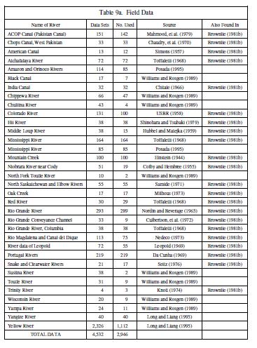
77 67

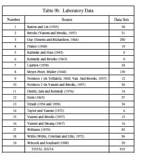
78 68

79 69 Table 1. Summary of 12 Sediment Transport Relations Correlation Coefficient Analysis of 10 Selected Equations The correlation coefficient Cc was calculated comparing Cppm computed to Cppm measured for the 10 selected equations. The equation for the correlation coefficient is C c If Cc is used for measured and computed Xi = computed sedimentation Yi = measured sedimentation ( X i X )( Yi Y) (31) 2 2 ( X X ) ( Y Y) X = average of computed sedimentation Y = average of measured sedimentation In the computation of Cc for Laursen and Bagnold: Xi = computed sedimentation, Laursen Yi = measured sedimentation, Bagnold i i

80 70 In addition, the correlation coefficient for hydraulic data, channel geometry parameters and sediment characteristics was conducted to determine the relative importance of variables affecting the accuracy of the 10 selected equations on calculated versus measured Cppm. The results of this analysis are given in Table 12. Many of the selected 10 equations were derived principally from laboratory data and the following comparison relies principally on field and laboratory data. There exists close correlation between selected relations. The correlations of Brownlie and Shen & Hung for three subdivisions of bed material are illustrated in Fig. 20. Figure 20. Correlation between Brownlie and Shen and Hung Equations.

81 71 The best variables to compute Cppm are velocity u, slope Sw, shear stress, and shear velocity u*. These variables are all closely related but depending on magnitude of flow the value of Sw is most difficult to measure accurately Total Load Equations Based on Advection-Diffusion, Energy Balance and Stream Power Concepts The equations based on energy and power concepts (six equations) and based on regression analysis (four equations) were tested and applied to alluvial rivers with a wide variety of sediment characteristics and hydraulic geometry data. The results from these equations were compared to field data, Kodoatie (1999) Einstein s Method Einstein (1950) initiated the indirect approach of determining the bedmaterial load by summing up the bed load and the suspended load. He was also among the first to introduce the idea of effective shear stress and computation by size fraction. The total shear stress is considered to consist of two parts: the shear stress associated with grain roughness ' and the shear stress associated with form shear stress ''. ' " (32) The grain shear stress is most effective relative to the transport of sediment and it is the shear stress that would yield the mean velocity if all the resistances

82 72 were due to grain roughness. For the known values of velocity and hydraulic radius (or depth in the case of large width-depth ratios), the effective shear stress can be computed directly from any assumed velocity equation and grain roughness parameter Statistical Approach A comparison between computed results and field data was conducted and examined. From this comparison, ranking for the best fit from the sediment relations was tabulated. There are many different statistical parameters that can be used to test the goodness of fit of equations and different results can be obtained by selecting different statistical parameters (Yang, et al., 1996) Analysis of Sediment Transport Relations The field data were divided into two categories: Group 1 for analysis of the selected sediment transport relations and proposed equations, and Group 2 for verification and validation of the proposed methods (Kodoatie, 1999). The river data sets were divided into two parts in random order. A comparison between computed results and field data was conducted and examined. Statistical approaches were used including the mean discrepancy ratio D R (Bechteller & Vetter, 1989; Wu, 1999; Nakato, 1990; Yang & Wan, 1991; and Hydrau- Tech, Inc., 1998), standard deviation D (Yang and Wan, 1991 and Hydrau-Tech, Inc., 1998), scattering of the discrepancy ratio s (Bechteller & Vetter, 1989), and the correlation coefficient CC, see Eq. 47, (Hydrau-Tech, Inc., 1998). The equations for each parameter follow: R D R X i i Ri (33) ' N Yi D log s ( R i R) N 1 1 X log N Y i i 2 (34) (35) For perfect fit, those values in Eqs. 30 through 32 are 1 D R, D = 0, s =0, and Cc = 1, refer to Eq. 28 for the value of Cc.

83 Applicability of Selected Sediment Transport Relations Fifteen other researchers evaluated the sediment transport relations, including: Alonso et al. (1982), Bechteler and Vetter (1989) Brownlie (1981a), Lau and Krishnappan (1985), Mau and Brooks (1991), Nakato (1990), Stevens and Yang (1989), Raphelt (1996), Rijn (1984), Vanoni (1975), White et al. (1975), Williams (1995), Wu (1999), Yang and Molinas (1982), and Yang and Wan (1991). Based on the results of these comparisons and the results of the present study by the authors, an attempt to identify the applicability of the 10 selected sediment transport relations was conducted Summary of Applicability of 10 Sediment Relations Analyzed As stated previously, the 10 sediment transport relationships were investigated (Kodoatie, 1999) to determine their applicability to four sizes of bed material and three sizes of rivers. The applicability of the 10 selected sediment transport relations, based upon comparison between measured and computed sediment transport rates, is summarized in Table 12 regarding the coefficient of correlation and Table 13 regarding the mean discrepancy ratio. The values of D R were computed considering the seven classifications of alluvial rivers, and the table gives the D R values for the 10 equations analyzed. The best equations for size of riverbed material are highlighted with one asterisk and the best equations for size of river are highlighted with two asterisks. Referring to the table, it is observed that the Laursen Equation is best for medium-tocoarse sand-bed rivers. The following conclusions can be drawn from the results of the statistical analysis (Kodoatie, 1999). 1. Gravel-bed rivers (2 mm < d50 < 64 mm) Compared to measured values, none of the selected sediment relations can accurately predict sediment discharge. The closest values based upon the discrepancy ratio were Ackers and White with D R = 0.33 and Brownlie with D R = However, based upon the Pearson correlation coefficient for comparison of computed to measured Cppm, the best equations were Bagnold and Shen and Hung, both with Cc of 0.71, Table 12. Considering gravel-bed rivers, Brownlie s equations although developed for sandbed rivers, were the most acceptable of the 10 equations, Table 13.

84 74 2. Medium to very coarse sand-bed rivers (0.250 mm < d50 < 2.00 mm) For this type of bed material, Toffaletti with D R = 0.93, Laursen with D R = 0.60, and Bagnold with D R = 1.68 compute Cppm closest to measured values. On the other hand, based upon the Pearson correlation coefficient, Karim with Cc = 0.66 followed by Brownlie with Cc = 0.60 best correlated with measured concentrations of bed-material discharge, Table Very fine to fine sand-bed rivers (0.062 mm < d50 < mm) The most suitable equations for bed material in this range were Karim and Kennedy with D R = 0.90, Karim with D R = 1.28, Table 12; Brownlie with Cc = 0.58, and Toffaletti with Cc = 0.52, Table Silt-bed rivers (0.004 mm < d50 < mm) For silt-bed rivers, Einstein with D R = 1.06, Bagnold with D R = 0.56, Toffaletti with Cc = 0.48, and Brownlie with Cc = 0.38 were the most acceptable relationships. 5. Small rivers (width 10 m and depth 1 m) The closest results obtained in small rivers is Brownlie with D R = 1.18, Karim with D R = 1.19, Yang with Cc = 0.85 and Toffaletti with Cc = Intermediate rivers (10 m < width 50 m and 1 m < depth 3 m)

85 75 For intermediate rivers, Toffaletti with D R = 0.94, Brownlie with D R = 0.94, Karim with Cc = 0.76, and Yang with Cc = 0.70 were the most acceptable relationships. 7. Large rivers (width > 50 m and depth > 3 m) For large rivers, Bagnold with D R = 1.04, Laursen with D R = 1.13, Brownlie with Cc = 0.80, and Shen and Hung with Cc = 0.76 were the most acceptable relationships. It should be noted that for silt-bed rivers and for very fine to fine sand-bed rivers, the Yellow River contributes about 77 percent and 63 percent of the data, respectively. As reported by many investigators, this river is an extremely heavily sediment-laden river and floods experience hyperconcentrations of sediment. Out of all rivers, this river system is unique and therefore should not be categorized as a common alluvial river. 8. Summary In summary, from the analysis it is evident that both Ackers and White and Toffaletti have a tendency to increase the computed concentration of suspended sediment, as the median diameter of bed material becomes finer. This tendency also occurs with these relationships when the river size increases. Additionally, the results of applying the 10 widely utilized relationships are presented in Figures 21 and 22. Note that the computed data, as compared with measured data, scatter widely, in fact, over several log cycles. Several of the primary difficulties limiting the use of these relationships is determining size and gradation of bed material, channel stability, sediment supply, aggradation, degradation, and the potential for armoring. As stated previously, Kodoatie (1999) and the authors conducted a thorough study of the identified transport relationships based upon the total database available, past studies, and observations from field studies. The three relationships that presented the best merits for improvement were selected and modified. The three relationships are: the Simons, Li & Associates Methodology, the Posada and Nordin Methodology, and the Laursen Equation and modified versions of the Laursen Equation. The results of this further analysis have been selected for presentation in this paper.

86 Figure 21. Computed versus measured total bed-material transport considering four classifications of size of bed materials, Kodoatie, (1999). 76

87 77 Figure 22 Computed versus measured total bed-material transport considering four classifications of size of bed materials, Kodoatie, (1999) Simons, Li & Associates Methodology The Simons, Li & Associates (1982) relationship is c s 2 c 3 q s 1 cs 1d u (36) where cs1, cs2, cs3, are coefficients based upon mean particle diameter (d50) ranging from sand to fine gravel (0.1 mm 5.0 mm). These equations have the advantage of being independent of energy gradient that is difficult to measure on intermediate and large, flat rivers. Table 14 provides the coefficient and

88 78 exponents for Eq. 33 for different gradation coefficients and sizes of bed material. The term G in Table 14 is defined as the gradation coefficient of the bed material and is 1 d 50 ds 4 G (37) 2 d16 d50 where d16 is equal to the size of the bed material for which 84 percent is coarser, etc. This is supported by Table 15 that identifies the coefficients utilized in the equation based upon size of sediment, gradation of sediment, and hydraulic conditions. Also, the range of data utilized to develop this relationship is presented in Table 15. Equation 33 was developed for steep, sand- and gravel-bed channels experiencing only critical and supercritical flows (Simons, et al. (1981), Julien (1995)). Arizona Department of Transportation funded the Simons, et al. analysis. This equation was analyzed and modified by the authors to obtain a sediment transport relation for various ranges of hydraulic geometry and sediment sizes.

89 Modified Simons, Li & Associates Methodology Considering the correlation coefficient for each variable of hydraulic geometry and the sediment characteristics, the Simons, et al. relationship was modified by the authors using nonlinear optimization and the field data for different sizes of riverbeds to become b c d q1 au h S (38) where a, b, c, and d are coefficients from Table 16, u is the average velocity, h is the depth and S is the slope of the hydraulic gradient. The coefficient and exponents in Table 16 are utilized in Eq. 35, depending on size and gradation of bed material based upon data from Group 1. The data were randomly divided into two groups: one group of data was used to develop the modified equation and the second group of data was used to validate the equations. It can be concluded from Fig. 23 that the Modified Simons, et al. equation shows an improved applicability to the four classes of channels. In general, the Posada Method is not applicable to gravel-bed rivers.

90 80 Figure 23. Comparison of qs measured and qs computed using Posada/Nordin and Modified Simons, et al. equations for four sizes of riverbed materials, data from Group 1, Kodoatie (1999) Posada and Nordin Methodology Posada (1995) and Nordin proposed a sediment discharge relation for large sand-bed rivers as a function of velocity 5 q1 30u (39)

91 81 where t q = the unit sand discharge (mg/m/day) u = the mean velocity (m/s) This simple equation verifies the strong correlation between velocity and bed-material transport, particularly if executed two-dimensionally. Discrepancy ratios and correlation coefficients for the Posada/Nordin and Modified Simons, et al. equation, based upon data from Group 1, are shown in Table 17. The comparison between the Modified Simons, et al. relation and the Posada/Nordin relation using the data from Group 1 for four categories of riverbed material are shown in Fig. 23a through 23d. Equations 35 and 36 were verified using data from Group 2. The discrepancy ratios and correlation coefficients are shown in Table 18. The comparison between the Posada/Nordin and the Modified Simons, et al. equations using the data from Group 2 for four categories of riverbeds is presented in Fig. 24a through 24d.

92 82 Figure 24. Verification of Modified Simons, et al., and Posada/Nordin for four sizes of riverbed material data from Group 2, Kodoatie (1999). Figure 25. Verification of Modified Simons, et al., and Posada/Nordin for four sizes of riverbed material data from Group 2, Kodoatie (1999) Laursen Equation (1958) Laursen (1958) working with Hunter Rouse developed the following equation. 7/6 ' d i o u. c pi 1 f (40) i d ci i

93 83 This relationship was adopted and revised by several scientists in an attempt to improve its applicability. The original Laursen Equation was modified by Madden (1985) as follows c di pb i d 7/6 ' o ci u f 0. i Fr (41) The Laursen Equation was further modified by Copeland and Thomas (1989). Their relationship is 7/6 ' d i o u. c pi 1 f (42) i d ci i Modified Laursen Equation 1 In the study conducted by Kodoatie and the authors, a statistical analysis of the importance of variables related to transport of sediment was conducted, as illustrated in Table 11. The improvement to the Laursen Equation yielded Eq. 39 as follows: 7/6 u. log ' d 50 o 50 c (43) d c50 The method of determining log ( / ) * f u can utilize the modified Laursen graph, Figure 25, or the equations for each size of bed material. These equations for rivers with silt beds, very fine to fine sand beds, medium to coarse sand beds and gravel beds are: Y L Ln( x) y Ln( x) (44) Y L Ln( x) (45) Y L Ln( x) (46) Y L Ln( x) (47)

94 84 in which Y L log f ( u./ ) x u./ Considering the various categories of investigation, the results of applying the above equation verifies the following. Figure 26. Relationship of u*/ i and log f(u*/ i) for four sizes of river-bed material diameter data from Group 1 and proposed modified Laursen graph. 1. Silt-bed rivers Most of the Cppm computed is greater than C ppm measured. The discrepancy ratio R D ranges from 0.5 to 2 for 48 percent of the data

95 85 sets, less than 0.5 for 19 percent, greater than 2 for 33 percent, and the R D ranges from 0.75 to 1.25 for 22 percent of the data. 2. Very fine to fine-bed rivers Most of the Cppm computed is smaller than Cppm measured. The C ranges from 0.5 to 2 for 19 percent of the data sets, less than 0.5 for 80 percent, greater than 2 for 2 percent, and the 1.25 for 7 percent of the data. R D ranges from 0.75 to 3. Medium to coarse-bed rivers Most of the Cppm computed is smaller than Cppm measured. The D R ranges from 0.5 to 2 for 20 percent of the data sets, less than 0.5 for 75 percent, greater than 2 is 5 percent, and the R D ranges from 0.75 to 1.25 for 6 percent of the data. 4. Gravel-bed rivers Most of the C ppm computed is larger than C ppm measured. The R D ranges from 0.5 to 2 for 15 percent of the data sets, less than 0.5 for 3 percent, greater than 2 for 81 percent, and the to 1.25 for 3 percent of the data. 5. Small rivers R D ranges from 0.75 Most of the C ppm computed is greater than C ppm measured. The R D ranges from 0.5 to 2 for 60 percent of the data sets, less than 0.5 for 20 percent, greater than 2 for 21 percent, and the D R ranges from 0.75 to 1.25 for about 23 percent of the data. 6. Intermediate rivers Most of the Cppm computed is smaller than Cppm measured. The R D ranges from 0.5 to 2 for 15 percent of the data sets, less than 0.5 for 85 percent, greater than 2 for 2 percent, and the D R ranges from 0.75 to 1.25 for about 5 percent of the data. 7. Large rivers Most of the C ppm computed is much smaller than C ppm measured. The R D ranges from 0.5 to 2 for 9 percent of the data sets, less than 0.5

96 86 for 83 percent, greater than 2 for 8 percent, and the D R ranges from 0.75 to 1.25 for 5 percent of the data. In summary, Table 19 documents the D R values for each of the four subdivisions of bed material. To illustrate the application of the Modified Laursen 1 Equation, the following problem is presented and solved. Application of Modified Laursen 1 Example Problem Problem Solution For a river at low flow, the following data were collected: w S = 3.04 E-0.5, u = 2.79 ft/sec, 50 d = d = ft, ' o c 2 V 58 d 50 d 1/ lbs / ft 4d lbs / sf The Modified Laursen 1 Equation is: 2 7/6 log u. d ' 50 o c (48) d c50

97 87 and 7/ C (62.4) , C 1 The concentration in ppm by weight is ppm ppm 3.07 which is a very small concentration Modified Laursen Equation 2 In a further attempt to improve the Modified Laursen Equation 1, Kodoatie (1999) and the authors investigated which of the three stream power functions best correlated with the transport of sediment. The analysis is presented in Fig. 26a through 26c.

98 88 Figure 27. Relations of Cppm (measured) with stream power, unit stream power, and dimensionless unit stream power, Kodoatie (1999). The investigation of stream power verified that the form of stream power us/was most strongly correlated with transport. The Modified Laursen Equation 2 incorporates the dimensionless unit stream power us/utilizing regression analysis and nonlinear optimization techniques. The Modified Laursen Equation 2 is C d 50 d 7/6 u. ' log o c50 a us (49) where the coefficient a is a variable related to mean bed-material diameter as shown in Table 20.

99 89 Note in the Modified Laursen Equation 2 that an exponent equal to f(u*/ 50) is a significant variable. This parameter can be determined referring to Fig. 25 or computed by the selected Eqs. 40 through 43. The modifications to the Laursen equation by Madden, Copeland and the authors are presented in Table 21. The results from applying the Laursen and the Modified Laursen Equation 2 follow. Medium to Very Coarse Sand-Bed Rivers Comparison between Cppm measured and Cppm computed by the Modified Laursen Equation 2 by the authors are shown in Figure 27 and Table 21.

100 90 Figure 28. Comparison Cppm measured and Cppm computed using Laursen and Modified Laursen Equation 2 for medium to very coarse, sand-bed rivers, Group 2. Data. Very Fine to Fine Sand-Bed Rivers Comparison between Cppm measured and Cppm computed by the Modified Laursen Equation 2 are shown in Figure 28 and Table 22. Figure 29. Comparison Cppm measured and Cppm computed using Laursen and Modified Laursen Equation 2 for very fine, sand-bed rivers, data from Group 2.

101 91 Silt-Bed Rivers Comparison between Cppm measured and Cppm computed by the Modified Laursen Equation 2 are shown in Figure 29 and Table 21. Figure 30. Comparison Cppm measured and Cppm computed using Laursen and Modified Laursen Equation 2 for silt-bed rivers, data from Group 2. The application of the Modified Laursen Equation 2 involves an additional term as compared to the Modified Laursen Equation 1. The Modified Laursen Equation 2 incorporates the concept of stream power and gives an additional refinement to the Modified Laursen Equation 1. In choosing between the application of the Modified Laursen Equation 1 and the Modified Laursen Equation 2, refer to the values of D R as documented in Table 21. The Modified Laursen Equation 2 is superior in most cases to the Modified Laursen Equation Verification of Modified Laursen 1 and 2 Equations Utilizing Data from Group 2 The data from Group 2 were utilized to test the validity of Laursen s Method, Modified Laursen 1 and Modified Laursen 2 Equations. For coarse, sand-bed rivers, the computed discrepancy ratio was 0.60 for the Laursen

102 92 Method, 0.98 for the Modified Laursen 1 method, and 2.35 for the Modified Laursen 2 method. For very fine to fine, sand-bed rivers, the computed discrepancy ratio was 0.36 for the Laursen Method, 1.32 for the Modified Laursen 1 method, and 1.01 for the Modified Laursen 2 method. For silt-bed rivers, the computed discrepancy ratio was 1.47 for the Laursen Method, 1.19 for the Modified Laursen 1 method, and 1.00 for the Modified Laursen 2 method. The only time that it is necessary to utilize the concept of routing by size fraction is when the gradation coefficient G is relatively large and transport of sediment from the bed can result in armoring of the bed. Refer to the subject of armoring presented after Beginning of Motion using the Shields Criteria. To illustrate the application of the Modified Laursen Equation 2, the following problem is presented and solved. Application of Modified Laursen Equation 2 Example Problem Problem Utilizing the Modified Laursen Equation 2 as follows, compute the concentration of sediment ppm by weight. Data: Q C = m2/sec, d = 2.31 m, V w = m/sec, = m Co = 14.44, d50 = 0.32 mm, Sw = , 1.16E-06 d 50 d 7/6 ' o c50 log u a us

103 93 Solution Estimated parameters: and and = m/sec 50 d = U U. log / C 1 (0.01)(62.4) 110 (0.0045) ppm ppm Site-Specific Equations The preceding analysis verifies the importance of subdividing all channels by size and gradation of bed material. Reviewing the coefficients D R and Cc, the most acceptable equations are the Modified Simons and the Modified Laursen Equations 1 and 2. For further improvement, it becomes necessary to develop site-specific equations based upon the geomorphology of the reach and/or collected data. To develop these relationships, the following paragraphs detail the procedure. Site-specific equations are equations generated by the user. In mathematical models, such equations are referred to as User-Supplied Equations. The motivation for developing site-specific relations for bed-material transport is: The characteristics of the reach of river are qualitative, particularly with respect to bed-material transport.

104 94 Very limited or no transport data are available for an important range of discharge for the reach. The engineering problem is sufficiently important, cost-wise and environmentally, that special attention should be given to the problem. With these conditions, the following procedures are recommended. Make a detailed geomorphically-oriented site visit. Classify the reach as to its size and type of bed material. Assess the stability of the reach both geomorphically and hydraulically. Select the transport equation that is applicable to the physical conditions and the data that are available. Determine the flow frequency using existing data. In some cases, there may be a short supply of flow data. In this case, synthesizing the necessary data is required. If the project is important, complex, and requires time to formulate an acceptable design or analysis, immediately organize a data collection program. This program would include collecting the following data: flow, supply of sediment, bed-material transport, gradient of the river, and size and gradation of bed material. Even a few months of data extending over one maximum runoff period is worthwhile. Document the hydrologic data pertinent to the design. Utilize the suspended and bed-load data that are available supplemented by newly collected data. Fit the selected bed load and suspended load equations to the transport data. For example, in a reach of river where the bed material ranges from sand to cobbles: Plot the flow versus existing suspended and bed load values as illustrated in Fig. 30. Modify these selected equations to best fit the data for both forms of transport. With the best fit equations for both suspended bed load and bed load, extend the selected transport relations to estimate the values of bedmaterial transport for the range of flows that must be accommodated in the design or analysis, i.e., Q100, Q200, etc. Next, add the ordinates of suspended bed-material transport and bedload transport to establish the curve representing total bed-material transport, as illustrated in Fig. 30. Fit a power relation to the total bed-material transport curve S 3 Q. This relationship should be introduced into the analysis as the user supplied equation.

105 95 Figure 31. Development of a user-supplied equation. To further illustrate this method, the following information is presented from an analysis conducted on the Skokomish River in the State of Washington, Simons & Associates (unpublished report). Transport data were collected and measured including both suspended load and bed load. The Skokomish River is predominantly a gravel- and cobble-bed river with silt and sand transported as wash load. In this case, a Helley-Smith Sampler was utilized to collect the bed load. The Skokomish River has experienced significant channel bed aggradation, frequent flooding, and potential avulsions. These changes are primarily the result of significant increases in coarse sediment produced by portions of the upstream watershed. Hydraulic and sediment transport data were collected in the field to better understand the dynamics of the river. A sediment transport model was then calibrated and applied to evaluate various factors and potential solutions to the issues faced by those who live along the river and who attempt to manage and regulate the river. The above procedure was followed. The user-supplied equation was utilized to calculate the bed-material load over the range of expected flow up to and including the 100-year event. The period of time over which flow, suspended load and bed load was collected was approximately three years. This period was relatively wet and several sets of data were collected at relatively high flow. Since silt and sand was largely wash load, only the gravel and cobble component of total sediment transport was of major concern. The equation of choice for the Skokomish River was the Meyer-Peter, Müller (1958) transport equation. This equation, Eq. 64, was selected because it was developed for coarse bed-material transport. Additionally, this equation is widely accepted in the United States and in Europe. It was necessary to select an equation that was accepted because this analysis involved litigation between the Skokomish Indian tribe and Tacoma Public Utilities. This equation was subjected to major

106 96 modifications to achieve acceptable calibration and verification of the output. Similarly, an accepted model for routing water and sediment was dictated to meet the objectives of the analysis from the engineering and litigation perspective. The model that was selected was HEC-2QS, Cunge, et al. (1980). The adapted Meyer-Peter, Müller (1948) equation was developed based on experiments with sand particles of uniform sizes, sand particles of mixed sizes and density, natural gravel, lignite, and barite. This equation is: Qb K Q K s r 3/ 2 1/3 2/3 ' s 2/3 ( s ) dm qb g s yos B (50) where B q = bed-load rate in weight per unit time and per unit width, Q b Q y o S f = water discharge quantity determining bed-load transport, = total water discharge, = depth of flow, = energy slope, and B, B = dimensionless constants. B has the value for sediment transport and for the case of no sediment transport. B has a value of 0.25 for sediment transport and is meaningless for no transport since B q is zero and the last term drops out. The quantities B K and r K are defined by the expressions and 2/3 1/2 u K B R S (51) 2/3 1/2 u Kr R S (52) where S f = total energy slope, S f = part of the total slope required to overcome grain resistance, and S f f S = part of the total slope required to overcome form resistance.

107 97 Therefore K K B r f 8 u grs b (53) f ' Where f b is the Darcy-Weisbach bed friction factor for the grain roughness. The coefficient ' b f is determined from the Nikuradse pipe friction data with pipe diameter equal to four times the hydraulic radius and 90 K d s. If the boundary is hydraulically rough, r (u d / v 100),K * 90 is given by 26 K r (54) 1/ 6 d 90 in which d 90 is in meters. Equation 45 is dimensionally homogeneous so that any consistent set of units may be used. Equation 45 has been converted to units generally used in the United States in the field of sedimentation for water and quartz particles by the U.S. Bureau of Reclamation (1960). This equation is 3/ 2 1/ 6 Q b d q B yos f dm (55) Q nb 3/ 2 where q B = tons per day per foot width, Q b Q = water discharge quantity determining the bed- in cfs, = total water discharge quantity in cfs, and d m, d 90 = in millimeters. The quantity dm is the effective diameter of the sediment given by

108 si i i m d d (56) where = percentage by weight of that fraction of the bed material with geometric mean size si d, The term nb is the Manning roughness coefficient for the bed of rectangular channels 2/3 2 3/ n n W y n n w o b (57) and for trapezoidal channels 3 2 / 2 3/ 2 1/ 2 1/ 1 ) (1 2 1 n n H y n n w s o b (58) where n, n, n = roughness coefficients of the total stream of the bed and of the banks, respectively, H s = horizontal side slope related to one unit vertically, and W = bottom width. The ratio Qb/Q for rectangular channels is given by 2 3/ b w o b n n W y Q Q (59) and for trapezoidal channels is 2 3/ 2 1/ b w s o b n n W H y Q Q (60) The Meyer-Peter, Müller formula (Eq. 45) is often written in the form 2 3/ c b K q (61)

109 99 where: and K B g 1 s s 3 / 2 1/ 3 2 / s (62) where: Q K 3/ 2 b B yos f Q K (63) r c s d m B ' (64) Since the ability to measure shear stress has a high degree of uncertainty, it was determined to utilize velocity, as related to shear stress, to calculate the average shear stress on the bed. This equation is: 2 fu o (65) 8 where f = the Darcy-Weisbach resistance coefficient = the mass density of water, and U = the average velocity in the channel. The Manning s equation was utilized to define the average velocity in the channel. The Manning s n-values were varied at each cross section in order to obtain an optimum fit between measured and computed velocities. The computed and measured velocities are presented in Fig. 31 at the Highway 101 Bridge and Fig. 32 at the Highway 106 Bridge.

110 100 Figure 32. Skokomish River computed and measured velocities at Highway 101 Bridge, Simons & Associates (2001). The critical shear stress is based upon a Shields parameter c 0.01 d s s (66)

111 101 Figure 33. Skokomish River computed and measured velocities at Highway 106 Bridge, Simons & Associates (2001). The Skokomish River is historically, dating from 1946, a slowly aggrading river due to deforestation in the upper watershed. This value of Shields parameter was necessary to create sufficient differential shear between actual shear and critical shear to calibrate Meyer-Peter, Müller with measured bed load. In order to obtain a best fit of the Meyer- Peter, Müller equation to the measured data, it was necessary to adopt a variable exponent to the simplified equation, which is where the value of x is q c o x c K (67) ( ( u3)) x (68) The resulting modified Meyer-Peter, Müller equation applied to size fractions of the bed sediment is q ) x c ( o c (69) This modified equation was utilized in the HEC-2QS model to route the water and sediment in the Skokomish River. The routing period was 50 years. The

112 102 comparison of measured with computed bed load is shown in Fig. 33 for the Highway 101 Bridge. Similarly, the comparison of measured with computed bed load is shown in Fig. 34 for the Highway 106 Bridge. In addition to computing transport rates, comparison of measured and computed sizes of bed material were made to further calibrate and verify the model. Figure 34. Skokomish River comparison of measured with computed bed load at Highway 101 Bridge, Simons & Associates (2001).

113 103 Figure 35. Skokomish River comparison of measured with computed Qs bed load at Highway 106 Bridge, Simons & Associates (2001). In addition to the sediment and water discharge data collected on the Skokomish River, samples of water and sediment were calculated on the South Fork of the Skokomish River. Upstream at Section 1, shown in Fig. 35, the South Fork of the Skokomish River is the principle source of sediment for the Skokomish River. Adjustments to these measured values were added to observed water and sediment discharge measured at Section 1 to account for the ungaged portion of the watershed and the ungaged portion of the bed-material load. Figure 35 illustrates that the Skokomish River is significantly aggradational as we observe computed bed-material transport from Section 1 to Section 36.

114 104 Figure 36. Skokomish River total bed load at Sections 1 through 36, Simons & Associates (2001). The quantity of bed load transported, used as upstream supply, and totaled approximately 2.2 million tons over 50 years. The quantities of bed load transported past the 101 and 106 bridges were significantly less (approximately 800,000 and 450,000 tons, respectively). These decreasing quantities of sediment transported (shown on Fig. 35) are an indication of channel bed aggradation, due primarily to the decreasing riverbed slope as the river approaches its delta and the Hood Canal estuary. These tonnages of sediment deposition closely correlate with the depth of channel bed elevation change based on the shift in rating curve at an available stream gage and with cited comparisons of channel bed elevation based on topographic maps over time Limitations of Modified Equations These modified equations, as presented in this paper, estimate total bedmaterial transport. The majority of the field data on transport of bed material consists of measured suspended sediment load, Benedict, et al. (1955). To correct this deficiency, the following procedure is recommended when using modified equations for sand sizes of bed material. For small, sand-bed rivers with average velocities in excess of 3.5 fps (upperregime flow conditions), add 50 percent of the computed transport rate to estimate total bed-material transport.