Slip in the Canterbury earthquakes, New Zealand

Transcription

1 JOURNAL OF GEOPHYSICAL RESEARCH, VOL. 117,, doi: /2011jb008868, 2012 Slip in the Canterbury earthquakes, New Zealand J. R. Elliott, 1 E. K. Nissen, 2 P. C. England, 1 J. A. Jackson, 2 S. Lamb, 3 Z. Li, 4 M. Oehlers, 5 and B. Parsons 1 Received 13 September 2011; revised 23 December 2011; accepted 27 December 2011; published 3 March [1] The 3rd September 2010 Mw 7.1 Darfield and 21st February 2011 Mw 6.3 Christchurch (New Zealand) earthquakes occurred on previously unknown faults. We use InSAR ground displacements, SAR amplitude offsets, field mapping, aerial photographs, satellite optical imagery, a LiDAR DEM and teleseismic body-wave modeling to constrain the pattern of faulting in these earthquakes. The InSAR measurements reveal slip on multiple strike-slip segments and secondary reverse faults associated with the Darfield main shock. Fault orientations are consistent with those expected from the GPS-derived strain field. The InSAR line-of-sight displacement field indicates the main fault rupture is about 45 km long, and is confined largely to the upper 10 km of the crust. Slip on the individual fault segments of up to 8 m at 4 km depth indicate stress drops of 6 10 MPa. In each event, rupture initiated on a reverse fault segment, before continuing onto a strike-slip segment. The non-double couple seismological moment tensors for each event are matched well by the sum of double couple equivalent moment tensors for fault slip determined by InSAR. The slip distributions derived from InSAR observations of both the Darfield and Christchurch events show a 15-km-long gap in fault slip south-west of Christchurch, which may present a continuing seismic hazard if a further unknown fault structure of significant size should exist there. Citation: Elliott, J. R., E. K. Nissen, P. C. England, J. A. Jackson, S. Lamb, Z. Li, M. Oehlers, and B. Parsons (2012), Slip in the Canterbury earthquakes, New Zealand, J. Geophys. Res., 117,, doi: /2011jb Introduction [2] The 3rd September 2010 (UTC 16:35, local time 04:35 on 4th September), Mw 7.1, Darfield earthquake occurred in the northern Canterbury Plains between 40 and 80 km west of the city of Christchurch (Figure 1). That earthquake caused no loss of life, but less than 6 months later (on the 21st February 2011 UTC 23:51, local time 12:51 on 22nd February) a smaller earthquake (Mw 6.3) occurred immediately beneath the city. Despite New Zealand s high standard of building codes, the extreme ground shaking caused building collapse that resulted in 182 deaths. Prior to the earthquakes, the principal seismic hazard for the region was presumed to arise from the major, mapped faults to the north and north-west in the Southern Alps and the Marlborough Fault Zone. The faults that ruptured in the 2010 and 2011 earthquakes were previously unknown. Preliminary studies have already either mapped the surface ruptures [Quigley 1 COMET+, Department of Earth Sciences, University of Oxford, Oxford, UK. 2 COMET+, Department of Earth Sciences, Bullard Laboratories, Cambridge, UK. 3 Institute of Geophysics, Victoria University of Wellington, Wellington, New Zealand. 4 COMET+, School of Geographical and Earth Sciences, University of Glasgow, Glasgow, UK. 5 Fugro NPA, Edenbridge, UK. Copyright 2012 by the American Geophysical Union /12/2011JB et al., 2010], geodetically constrained the main fault segments [Beavan et al., 2010] or determined the distribution of aftershocks [Gledhill et al., 2011]. We combine Interferometric Synthetic Aperture Radar (InSAR) observations (Figure 2), with field mapping, aerial and satellite imagery, a post-earthquake LiDAR Digital Elevation Model (DEM) and seismological body-wave solutions to examine the distribution of rupture, and to model the locations and orientations of these previously unknown faults. We show that the ruptures which occurred in these earthquakes form a complex array of faulting, but are consistent with the distributed interseismic strain of the region that had already been determined by GPS measurements [Wallace et al., 2007]. [3] The city of Christchurch and the Canterbury Plains lie to the east of the Southern Alps (Figure 1). The basement geology of the northern half of the plain consists of Triassic sandstones overlain by 1 km of nearly flat-lying Palaeocene and Eocene sandstones/mudstones, which are in turn overlain by up to 1 km of Pliocene-Pleistocene sediments [Forsyth et al., 2008]. The hilly topography of the Banks Peninsula to the south-east of Christchurch consists of Miocene basaltic lava flows. The Canterbury Plains has had no significant seismicity (Mw 5.5+) in the last five decades as recorded by the Engdahl catalogue [Engdahl and Villaseñor, 2002] (Figure 1), nor in the period (Mw 5.7+) examined by Doser et al. [1999] and was generally [Stirling et al., 2002] considered to be at a lower risk of earthquakes than other parts of New Zealand. The Late 1of36

2 Quaternary alluvial fan deposits that cover the region create a remarkably flat landscape (Figure 2a) and obscure any surface geomorphic evidence of faulting [Forsyth et al., 2008]. [4] In contrast, the Porter s Pass Fault system at the northwestern edge of the Canterbury Plains is clearly expressed in the topography, and the distribution of faulting is known in some detail (GNS Active Fault Database) [Forsyth et al., 2008]. Recent Global CMT solutions [Ekström et al., 2005] in the Porter s Pass Fault System indicate a pair of Mw 5.5 earthquakes in 1994 and 1995 at the edge of the Canterbury Plains, between the Waimakariri and Rakaia Figure 1 2of36

3 Rivers (Figure 1). The Porter s Pass Fault itself is thought to have a Holocene right-lateral slip rate of mm/yr and mm/yr on its eastern and western sections respectively [Howard et al., 2005]. [5] Faulting has recently (prior to the earthquakes) been revealed beneath the Quaternary cover in the north-western portion of the plains by seismic reflection profiling, which shows Cretaceous to Quaternary supracrustal rocks being faulted and folded [Dorn et al., 2010b]. Seismic profile lines running parallel to the Waimakariri River east of the Malvern Hills show numerous faults that probably represent northeastward extensions of mapped faults in the exposed Malvern foothills. Dorn et al. [2010a] had already suggested prior to the 2010 Darfield earthquake that faulting was likely to be distributed right across the Canterbury Plains, and that structures beneath the Canterbury Plains and neighboring regions have the potential to generate hazardous earthquakes. 2. Surface Rupturing in the Darfield Earthquake [6] In this section we describe the surface rupturing produced by the Darfield earthquake and determine variations in the sense and magnitude of surface slip along the length of the fault. We visited the area twice one of us (SL) shortly after the earthquake in September 2010, and two of us (SL and EKN) a second time in May We augment these field observations with an analysis of post-seismic remote sensing data, comprising Worldview satellite imagery (0.5 m resolution), orthorectified aerial photographs (0.25 m resolution) and a DEM with 2 m-resolution that was derived from airborne LiDAR after the Darfield earthquake. [7] The surface faulting disrupts a wide alluvial plain which slopes gently toward the SE, with an average gradient of Hillshaded LiDAR topography reveals an abundance of subdued fluvial landforms, with individual channels and bars typically showing relief of up to 0.5 m. These landforms were probably abandoned at the end of the last glaciation in the late Pleistocene [Forsyth et al., 2008]. Nowadays the landscape is intensely farmed, and contains an array of linear features roads, fences, hedges, ditches, plough lines and crop rows which allow the trace of the rupture to be easily identified and a dense set of offsets to be measured. [8] An initial summary of the ruptures was provided by Quigley et al. [2010], who observed 30 km of surface faulting along an E W trace, from 4 km west of Greendale (in the west) to 2 km north of Rolleston (in the east). The authors called this newly recognized fault the Greendale Fault. The westernmost 5 km of the rupture trends WNW ESE, approximately following the course of the Hororata river and in one place partially blocking its channel, leading to minor flooding of adjacent fields [Quigley et al., 2010, Figure 5]. However, this westernmost part lacks coverage of Worldview imagery, aerial photography or LiDAR topography. In the remainder of this section, we restrict our analysis to the area between Greendale and Rolleston, for which all of the high-resolution data-sets are available. [9] Surface rupturing in this area can be traced from 1 km south of Greendale (in the west) to 2 km north of Rolleston (in the east), a total distance of 22.5 km (Figures 2a and 3a). The overall trend of the rupture is 084, but in detail the surface faulting deviates from this azimuth, striking E in the western and eastern sections but ENE in the central part. We also inspected farmland and roads north of the Greendale Fault for signs of rupture on antithetic or splay faults, but found no evidence for surface slip in this area Horizontal Displacements [10] Along the Greendale Fault, rupturing has produced clear, right-lateral displacements to roads, fences, and other linear features (Figure 4). As pointed out by Quigley et al. [2010], the total strike-slip displacement is usually accommodated over a broad, m wide zone, rather than on a discrete fault trace, although the authors did not quantify the azimuth of the slip vector. This displacement zone is characterized by dense Riedel shear (R and R ) structures, although offsets on these discrete fractures can typically account for only a small percentage of the total strike-slip displacement [Quigley et al., 2010]. [11] We measured the right-lateral displacements of more than 70 individual linear features along the Greendale Fault (Table 1). These sites are plotted in Figure 3b, colored according to whether offsets were measured in the field (yellow), from aerial photographs (blue), from WorldView imagery (red), or from more than one of these methods. To ensure that we determined the full slip magnitude, we only used features that crossed the entire displacement zone and measured the cumulative offset across that full width. [12] In the field, it was easiest to measure offsets in the direction perpendicular to the azimuth of a particular feature. We repeated these measurements in map view using the remote sensing imagery, tracing parallel lines along linear features either side of the displacement zone. This use of the remote sensing imagery was in places limited by forest cover or shadow or by glitches in the aerial photography; in addition, the 50/25 cm pixel sizes made it difficult to resolve small displacements at the ends of the fault. Where we were able to use more than one method to measure the same Figure 1. Active fault map, earthquakes, topography and place names of the northern half of the South Island of New Zealand, covering the recent earthquake epicentral regions of Darfield and Christchurch at the north end of the Canterbury Plains. Focal mechanisms are from the GCMT catalogue for the 2010 and 2011 events studied here (black) and earthquakes Mw 5.5+ (grey) covering the period [Ekström et al., 2005]. Earthquake epicenters from the Engdahl catalogue [Engdahl and Villaseñor, 2002] are shown by grey circles. The active faults (black lines) are from the Institute of Geological and Nuclear Science (GNS) Active Faults Database. The main Alpine Fault and faults of the Marlborough Fault Zone (Hope, Clarence, Awatere and Wairau Faults) are marked to the north of Christchurch. Grey dashed outlines indicate the footprints of InSAR coverage for the three ascending and one descending ALOS tracks. The white arrow indicates the 40 mm/yr of relative motion of the Australian Plate relative to the Pacific Plate based upon the MORVEL motion [DeMets et al., 2010]. The inset map indicates the region of study (blue rectangle), plate boundaries (red) from Bird [2003], relative plate velocities (mm/yr) at the tips of New Zealand and the MUVEL pole of rotation [DeMets et al., 2010]. 3of36

4 Figure 2 4of36

5 displacements, we find good agreement between the different methods, with differences in offset normally <50 cm and always <1 m. [13] Strike-slip offsets were then estimated by converting perpendicular offset of the measured feature onto an E-W fault trace. The resulting strike-slip offsets are plotted as triangles in Figure 3d, colored according to the data used. However, this method of determining the right-lateral offset relies on an assumption that motion on the fault is purely strike-slip. In reality, any component of shortening or extension on the fault will also contribute toward the apparent offset. To investigate this, we focused on 23 locations where we could measure the apparent offsets of at least two displaced features lying in close proximity but with different orientations. By combining each pair of observations, we were able to calculate both the orientation and magnitude of the horizontal slip vector (details of this method will be provided by S. Lamb et al. (manuscript in preparation, 2012)). These horizontal slip magnitude measurements are plotted as circles in Figure 3d, and the slip vectors are plotted in Figure 3c. [14] The slip vectors determined in this study are consistent with predominantly strike-slip motion, and appear to track the local strike of the fault, with E-directed slip vectors in the west and east, but ENE-directed slip vectors along the central section. Horizontal slip magnitudes are 2 3 m in the west (with an average slip vector azimuth of 100 ), 4 5 m along the 6 km central section (078 ), 2 3 m further east and 1 m in the far east (103 ). In a few places, we observe a rapid change in horizontal slip magnitude over a short distance (e.g. 3 m over a distance of 400 m between sites 10 and 11), suggesting that in places some of the slip at depth fails to reach the surface, or that there are slip patches separated by areas on which creep had occurred Vertical Displacements [15] The displacement zone also corresponds to a topographic high, with relief of a few centimeters, up to a maximum of 0.5 m. Although this height difference is almost imperceptible on the ground, artificially illuminated LiDAR topography reveals a ridge that is divided into distinct, leftstepping mound structures (Figure 3). These vary in size, from a few meters in the smallest cases up to 50 m wide and 100 m long in the largest. These elongated mounds are aligned into discrete fault segments, usually m in length, separated by broad, left-stepping relay zones, typically m wide. Individual fault segments trend between 080 and 113, with an average of 093, and lie at a slight angle to the overall trend of the Greendale Fault (which is 084 ). The distinct length-scale of these segments may be controlled by the thickness of Quaternary alluvium underlying the rupture, which is also likely to be a few hundred meters. [16] Cross-fault elevation profiles measured from the LiDAR topography show that the fault zone accommodates a clear step in the surface elevation (Figure 5), providing further evidence for a small dip-slip component to the faulting. This step is always up to the south reversing the prevailing regional slope, which is to the SE and is observed across both the en echelon fault segments and the left-stepping relay zones. The steps are preserved across road surfaces and fields that are likely to have been flat prior to the earthquake, and it is likely that they formed during the Darfield event alone, rather than cumulatively through multiple past earthquakes. For forty profiles in which the surface gradients either side of the fault can be matched (usually those confined to a single field or road surface), the height of the step can be estimated. The distribution of vertical offsets is shown in Figure 5 and Table 2, and we estimate typical uncertainties of 10 cm in these measurements. In the main part, vertical offsets are <0.5 m. The largest vertical displacement, of 1.4 m, occurs next to an abruptly change in strike from E to ENE, and is probably related to transpression within this restraining bend. [17] It should be noted that there are also variations from this general description of the Greendale Fault ruptures. In the west, a 1.5 km section of ruptures comprise a clear scarp (up to the south) but show no discrete mound structures. The easternmost 5 km of the ruptures, which are separated from the rest by a larger left-step of 1 km, show neither a scarp nor ridges, indicating that faulting here is probably purely strike-slip. 3. Teleseismic Body-Wave Modeling [18] We used teleseismic body-waveform modeling to obtain independent estimates of the source parameters of the Mw 7.1 Darfield and Mw 6.3 Christchurch earthquakes, as well as for the most recent June 2011 Mw 6.0 aftershock. The methods used are described in Appendix A. As they generated small signals compared with the noise, we could not obtain solutions for the two Mw aftershocks listed in the GCMT catalogue three days after the Darfield event (Figure 6), nor for the pair of Mw aftershocks Figure 2. (a) SRTM derived hillshade DEM map (artificially illuminated from the SE) centered over the Darfield earthquake epicenter, with main population centers marked. The spatial extent of the surface rupture mapped in the field is denoted by the east-west red line. No obvious surface expression of the fault is visible in the surface geomorphology. (b) Interferometric fringes rewrapped to 12 cm from the descending ALOS interferogram on track 631. A color cycle from blue through yellow to red indicates motion of 24 cm away from the satellite in the line-of-sight (los). Black arrows indicate the satellite azimuth direction (Az) and the line-of-sight (los) look direction with the angle of incidence (i) also given. (c) As in Figure 2b for ascending ALOS interferogram on track 336. (d) As in Figure 2b for ascending ALOS interferogram on track 337. (e) ALOS azimuth offsets for track 337A. Positive values are in the direction of satellite motion (NNW). The main east-west fault trace is clearly visible as the change in offset (delineated by black arrows). Additionally a change in azimuth offset is seen running NNW from the main fault (denoted LL). (f) ALOS range offsets (track 337A) (motion away from the satellite reckoned positive). The east-west fault trace is clearly visible as a change in offset of almost 4 m, with a change in strike seen for the western-most portion. Additionally, a sharp discontinuity in the offsets is seen striking NNE from the main fault trace (denoted TH). 5of36

6 Figure 3. (a) Shaded 2 m-resolution LiDAR topography along the main Darfield earthquake rupture (LiDAR data does not cover the westernmost part of the rupture, W of Greendale). Red arrows pick out the ends of the main rupture sections. (b) Locations where we were able to measure horizontal (numbered every ten to match those in Table 1) and vertical offsets (indicated by a P and numbered to match those shown in Figure 5 and Table 2). (c) Variations in the horizontal slip vector along the rupture. (d) Longitudinal profile showing variations in horizontal (circles) and vertical (squares) slip magnitude. 6of36

7 Figure 4 7of36

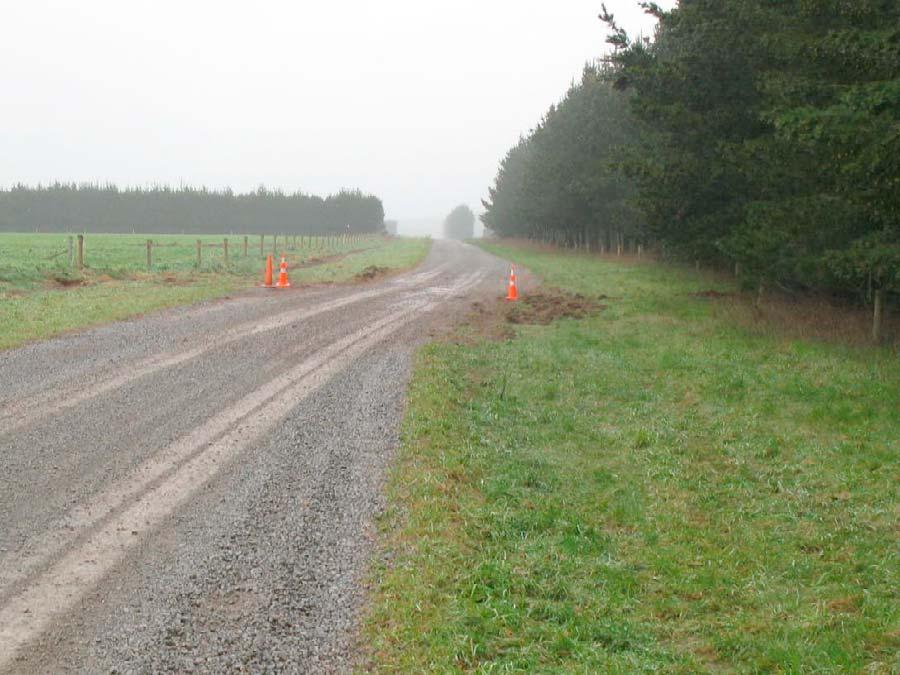
8 as they closely followed in the minutes/hours after the Christchurch earthquake. [19] The body-wave solution for the Darfield earthquake (Figure 7) is consistent with an east-west striking, steeply south-dipping, right-lateral rupture, and has a similar mechanism to the best-fitting double couple GCMT solution (Table 3), but with a shallower centroid depth of 7 km. The body wave solution is expected to have better centroid depth resolution than the GCMT, but has a typical uncertainty of 3 km due to trade-offs with the source time function, which also affects the moment. The calculated moment is Nm, equivalent to a moment magnitude of Mw 6.9, 70% of that of the GCMT solution and 40% of the regional moment tensor solution from GeoNet [Gledhill et al., 2011], which has a centroid depth of 8 km. The source time function is about 15 s, consistent with km of faulting, assuming bilateral rupture and a rupture speed of about 2.5 km/s. [20] The Christchurch earthquake has a body-wave solution (Figure 8) that indicates highly oblique reverse/dextral faulting on a NE-SW striking plane (assuming a SE rather than west-dipping fault plane solution based upon the distribution of aftershocks; Figure 6). The centroid depth is shallow at 4 km and has a moment of Nm (Mw 6.2), one tenth of the Darfield moment. The source time function is about 6 s, indicating almost 15 km of rupture. The body-wave solution is most consistent with the GeoNet solution in terms of fault parameters, centroid depth and moment release (Table 4), whereas the GCMT and USGS solutions indicate greater strike-slip motion and an ENE- WSW strike. 4. Fault Geometry of the September 2010 Darfield Earthquake [21] We use phase measurements from ALOS interferograms (Figures 2b 2d and Table 5) to constrain the geometry of faulting and the distribution of slip, and compare them to the previously published model by Beavan et al. [2010]. The methods to generate the interferograms, down-sample the data and model the fault slip [e.g., Wright et al., 1999] are given in Appendix B. [22] The combination of phase measurements, range and azimuth offsets (Figure 2), field data (Figure 3a) and aftershock distributions (Figure 6), all point to a minimum of 8 segments to satisfactorily fit the observations (Table 3). We attempted solutions with fewer segments, but all such models left systematic misfits in the InSAR data. With this degree of complexity, it is computationally prohibitive to explore the full space of 9 fault parameters for each segment simultaneously. However, field and InSAR measurements place tight constraints on the fault segmentation and positioning. We use those observations to fix the locations, lengths and strikes of the individual segments, reducing the number of unknowns. [23] Field observations of surface rupture required two main east-west, predominately strike-slip fault segments (numbered 2 and 4 in Table 3 and Figure 9), which step leftward and are connected by a NNE-SSW striking segment (3). This configuration is supported by the linear patches of incoherence in the InSAR data (in particular for track 337A; Figure 2d) and by the range and azimuth offsets (Figures 2e and 2f). The SAR offsets and interferogram incoherence patterns also require a continuation of the fault striking WNW from the western edge of the main mapped east-west rupture (segment 1), beyond where any evidence of surface offsets was found in the field. [24] Segment 5 is required to the east of Rolleston to fit the eastern-most fringes in the descending ALOS data (Figure 2b), and which are also evident as a single lobe in the phase data for the ascending tracks (Figures 2c and 2d). However, east of Rolleston, there is no evidence of a surface trace in the field observations, indicating this segment comprises buried slip. We also note a NW trending signal in the ALOS azimuth offsets (marked LL in Figure 2e), which is consistent with left-lateral motion and for which we define the location and strike of segment 6. [25] Secondary fault segments (7 and 8) are required at high angles to the main strike-slip segments (2 and 1 respectively) to explain the bull s eye pattern of phase in the west of the track 631 and track 337 interferograms, as well as the high phase gradients in the center of the interferograms, immediately north of the main east-west rupture. The predominantly east-west segments, separated by crosscutting faults, are also evident in the aftershock locations from GeoNet (Figure 6) Uniform Slip Modeling [26] We fix the strikes and locations of the centers of the segments, as given in Table 3, using the above set of observations. In addition, we fix segment lengths to that of the rupture and fixed the top depth to zero on the central segments (2, 3, 4) where the surface trace of the fault rupture has been mapped. We then iteratively vary the dip, rake, slip and bottom depth (as well as the top depth of those segments where there is no field evidence of surface rupture), segment by segment and generate forward models of the interferograms to determine the goodness of fit. We then fix the rake and slip for each segment to the values given in Table 3, and perform an inversion as described in Appendix B to find the best fit dips and bottom depths for each segment. [27] A model with uniform slip on each separate segment (Table 3) fits the three interferogram tracks of data (Figure 10) with an overall RMS for the down-sampled data points of 9.0 cm (individual track RMS values are given in Table 5). The residuals indicate that the long wavelength deformation has been accurately modeled, although a couple Figure 4. (a) Field photograph looking SSW of observed ground rupture and right-lateral offset of 4.1 m (Site 13B, Table 1). (b) Worldview-2 satellite image (0.5 cm resolution, false color bands RGB) of field location shown in Figure 4a. The road offset is clearly visible running north-south with a remotely measured dextral offset of 5.1 m. The pair of black arrows show the rupture running eastward through the field. (c) Field photograph looking NE of observed ground rupture and right-lateral offset of 2.3 m (Site 41A). (d) Aerial image (0.25 m resolution) of the location shown in Figure 4c, with a remotely measured road offset of 2.4 m. (e and f) Field photographs of right-lateral offset fences and hedges along the Darfield rupture, two days after the earthquake. 8of36

9 Table 1. Estimates of Surface Slip Magnitude and Slip Vector Along the Greendale Fault a Site Longitude Latitude Feature Azimuth? Offset (m) Horiz. Slip (m) Slip Vector fld aer sat fld aer sat fld aer sat fence fence A road B road hedge A hedge B hedge road A track B fence A road B track A fence B hedge A fence B fence A hedge B fence A fence B track A fence B road track fence A fence B fence ditch track fence fence A road B trees A trees B road fence fence fence crops A road B trees fence A fence B hedge hedge hedge A hedge B hedge A hedge B fence crops plough A fence B hedge A hedge B ditch hedge plough A hedge B road A road B path A path B hedge fence fence fence fence fence fence fence of36

10 Table 1. (continued) Site Longitude Latitude Feature Azimuth? Offset (m) Horiz. Slip (m) Slip Vector fld aer sat fld aer sat fld aer sat ditch hedge road A road B fence A road B railway a? offset is the offset of a linear feature perpendicular to its azimuth, measured from field observations (fld), aerial photographs (aer) or WorldView satellite imagery (sat). Horiz. slip is the horizontal slip magnitude. This can be calculated directly in locations where two offset features lie in close proximity (e.g., combining 3A and 3B). Where only a single offset feature is available, we project the perpendicular offset onto an E-W fault and assume that slip is purely strike-slip; in these cases, the horizontal slip is shown in italics. Slip vector is the horizontal slip vector, calculated from pairs of perpendicular offsets. of fringes (equivalent to 24 cm of mis-modeled deformation) remain in the very near field (Figure 10). The residuals in the far-field on track 337A clearly indicate atmospheric noise trending NE-SW (Figure 10h). [28] The fault segment map and equivalent moment tensor solutions for the uniform slip modeling are shown in Figure 9, overlain on the aftershock distributions. Our fault segmentation model agrees well with the spatial distribution Figure 5. Example cross sections showing the determination of vertical offsets on profiles across the fault zone assuming a constant topographic gradient prior to the earthquake. Profiles are numbered to match those indicated in Figure 3. A full list of offsets measured is given in Table of 36

11 Table 2. Locations and Estimates of LiDAR Derived Vertical Offsets a Profile Longitude Latitude Offset (m) a Profiles are numbered west to east to match those given in Figures 3 and 5. of aftershocks. The central main three segments (segments 2 4 in Table 3), on which the greatest slip occurs, are nearvertical, dextral, strike-slip mechanisms. These segments comprise two-thirds ( Nm) of the total moment modeled, and are each equivalent to Mw events. The western most segment (1) is 15 km long and strikes WNW, dipping slightly to the north with a small normal component. The easternmost segment (5) dips steeply to the south and requires slip only over a narrow range, with a small normal component. The westernmost circular pattern of phase decrease is best modeled as a north-westward dipping reverse fault (segment 8). This configuration is consistent with the mechanism and location of a Mw 4.9 aftershock recorded by the GCMT catalogue 3 days later, but the InSAR moment for this segment is Nm, equivalent to an Mw 6.2 earthquake, which suggests that the slip on this segment took place principally during the main event. [29] The deformation to the north of the central part of the rupture is considerably more complex than in the equivalent region to the south. Whereas the range changes from track 337A show a smooth gradient in the south, there are clear east-west gradients in range change to the north of the rupture (Figures 2b and 2d). This deformation is best modeled as an eastward, steeply dipping reverse fault superimposed on the otherwise mainly dextral motion. The segment is only 4.3 km long, but its slip of 4.5 m (high for such a short fault length) is required by the large phase differences in the InSAR data. The fault geometry is in good agreement with the first motion solution for the main earthquake from GeoNet (Figure 9) which recorded a NE-SW striking pure reverse mechanism [Gledhill et al., 2011], and indicated that the earthquake rupture initiated on this reverse segment, triggering the bi-lateral major slip on the adjacent dextral faults. This also explains why the GeoNet epicenter location lies 7 km north of the main east-west rupture. [30] The fault parameters found here are in general agreement with the preliminary 6-segment model of Beavan et al. [2010], which was based upon InSAR and GPS observations. The principal differences between our solution and that of Beavan et al. [2010] lie in the fault segmentation in the east, where the ALOS azimuth offsets (which are sensitive to north-south lateral motion) indicate the presence of a buried NNW-striking left-lateral strike-slip fault (segment 6) (Figure 2e), not included in their model. The ground displacement due to this segment is not obvious in the InSAR phase measurements, because the ENE- and WNWlooking geometries of the ascending and descending paths of the ALOS satellite are relatively insensitive to north-south motion. Close inspection shows, however, that this fault can be followed as a discontinuity in the phase on tracks 631D and 337A (Figures 2b and 2d). This segment also follows the NNW trend of the aftershocks north of the main east-west rupture (Figure 6). The largest mismatches between the observed and modeled GPS data given by Beavan et al. [2010, Figure 2a] are either side of this segment, and the direction of mismatch in the horizontal direction indicates unmodeled left-lateral motion. [31] The fault areas and slips of the eight fault segments determined by InSAR can be converted into equivalent moments (Table 3), whose sum is Nm, approximately 50% greater than that of the Global CMT full moment tensor solution ( Nm). However, the GCMT seismic and total geodetic moment tensors show the same non double-couple source mechanism, suggesting that the seismic rupture involved all of the complex system of faults that we have mapped (Figure 9). We calculate the percentage double-couple component as 79% and 85% for the InSAR and GCMT solutions respectively (Table 6), using a definition from Jackson et al. [2002]. [32] The magnitudes of slip on some of the shorter fault segments in the Darfield earthquake are large (Table 3), resulting in slip-to-length (u/l) ratios of up to , in contrast with the range shown by most earthquakes [Scholz, 2002]. The slip-to-length ratio for the main portion of the fault (segments 1 5, 46 km long), which has an average slip of 3 m, is We calculate the stress drop (Ds) on the main contiguous segments (1 5) and the remaining individual segments using the relation Ds =2M 0 /(pw 2 L) for large strike-slip earthquakes [Scholz, 2002]. Taking the five main east-west dextral strike-slip segments together, the cumulative moment is Nm, total length is 46 km, and average width is about 10 km, yielding an average stress drop of 6 MPa. The stress drops range from 6 10 MPa (Table 3), and these large values are 11 of 36

12 Figure 6. (a) Topography of the Christchurch region with main population centers marked. The mapped surface fault trace (red line) runs west-to-east between Greendale and Rolleston. (b) Distribution of aftershocks ML 3+ post Darfield main shock (red circles) and post Christchurch up to 31st July 2011 (blue circles), scaled by magnitude, from GeoNet (GNS Science Focal mechanisms are for the pair of main shocks (black) from the GCMT catalogues with epicenters positioned from the GeoNet data. The aftershocks recorded by the GCMT catalogue are denoted by grey focal mechanisms. The western pair of Mw aftershocks occurred on the 6th September, 3 days after the main shock. The eastern pair of Mw aftershocks are from the 22nd February, 13 and 120 min after the first event. On the 13th June 2011, a Mw 6.0 earthquake occurred SE of Christchurch. (c) Interferometric range changes re-wrapped to 12 cm on track 337 for the Darfield earthquake and tracks 335/336 for the Christchurch earthquake. There is a km gap between the two areas of high deformation where little strain has been released. 12 of 36

13 Figure 7 13 of 36

14 Table 3. Fault Parameters for Segments as Derived From the SAR Interferometry and SAR Offsets, Teleseismic Body Wave Modeling and the Seismic Catalogues Best-Double-Couple Solution (GCMT, USGS, GeoNet) a Fault Segment Strike Dip Rake Slip (m) Lon Lat Length (km) Width (km) Top Depth (km) Bottom Depth (km) Centroid Depth (km) Stress Drop (MPa) Moment (10 18 Nm) Magnitude M w Slip Vector Darfield 3rd September 2010, InSAR Strike-Slip Faulting Segments Darfield 3rd September 2010, InSAR Reverse Faulting Segments Total Fix l Vary l Darfield 3rd September 2010, Seismological Solutions BW USGS GCMT GeoNet P Axis Azimuth a In the case of the Darfield event, only the fault dip and bottom depth were free to vary in the inversion. The stress drop (Ds) for the contiguous segments 1 5 (using an average width of 10 km) and the other individual segments is calculated from the segment moment M 0, width W and length L using the relation Ds =2M 0 /(pw 2 L)[Scholz, 2002]. The latitude/longitude locations for the faults are the centroid for GCMT, the Preliminary Determined Epicenter (PDE) for the USGS Body Wave solution (USGS) and the updip projections of the fault segment center to the surface for the InSAR solutions. likely to be indicative of long recurrence intervals [Kanamori and Allen, 1986; Kanamori and Anderson, 1975], or the development of a new fault Distributed Slip Modeling [33] We next fix the fault geometry on the eight segments as that derived from the uniform slip solutions described above, and allow the slip to vary on each segment. This additional complexity is warranted, as it is clear from the surface ruptures that the magnitude of slip changes along strike within each segment (Figure 3). The use of a finite fault model also allows us to lengthen the ends of the fault along strike as well as vary the rakes on each. [34] We extend all but the centrally bounded fault segments (2 4) along strike and all segments down dip to a depth of 15 km for the strike-slip portions and 10 km for the reverse, subdividing each segment up into 1 km by 1 km slip patches. We then solve for the two components (variable rake) of slip on each patch [Funning et al., 2005], as described in Appendix B. Values of slip on each patch can be found in the auxiliary material. 1 A significant reduction in the near-field residuals is clear (Figure 10) for the variable rake model, with an overall reduction in the RMS from 9 cm 1 Auxiliary materials are available at ftp://ftp.agu.org/apend/jb/ 2011jb to 5 cm. The largest residuals remain around the epicentral location of the earthquake where there are high phase gradients associated with the interaction of the eastward dipping reverse and east-west dextral fault. The down-sampled interferogram data, and the correspondingly sampled distributed slip model and residuals are given in Appendix B. [35] The fault slip distribution is shown in Figure 11. The peak dextral slip of 8 m occurs at a depth of 4 km on the central segment (2) with significant slip down to 10 km. Buried sinistral slip of over 1 m occurs over a large area of the left-lateral fault segment (6) that trends from the main rupture (segment 3) NNW toward Darfield. In between these two faults lies the reverse segment (7) that has a updip projection at Charing Cross (Figure 9). This region of slip (up to 4.5 m) accommodates motion of crustal material as it is squeezed between the two strike-slip faults. East of Rolleston, the slip extends only 5 km toward Christchurch and only to a depth 8 km (segment 5). In order to test if significant slip occurred toward Christchurch, we extended this fault segment further eastward. However, if a fault exists to connect the eastern end of the Greendale Fault and the fault that slipped near Christchurch in February 2011, the geodetic data indicate little or no slip on such a structure has occurred. [36] An assessment of the error in the distributed slip due to atmospheric noise in the interferograms is made by Figure 7. Darfield body-wave minimum misfit solutions from the inversion of P and SH body-waves for a point source in a half-space. Focal mechanisms show (top) P and (bottom) SH nodal planes in a lower hemisphere projection. Closed and open circles represent the P- and T-axes respectively. Waveforms for each station are plotted around the focal mechanisms in approximate azimuthal locations. Observed waveforms are solid and synthetic waveforms are dashed, while the vertical ticks mark the inversion window. The station code is to the left of each waveform, in vertical capital letters. The vertical bar and number beside each focal sphere is the amplitude scale for the plotted seismograms (in mm). The STF is the source time function, and the scale bar below it is the horizontal scale for the seismograms. The numbers in the header are strike, dip, rake, centroid depth (km), and moment (Nm) for the best-fit solution. 14 of 36

15 Figure 8. Christchurch body-wave minimum misfit solutions from the inversion of P and SH bodywaves for a single point source in a half-space. Rest of caption as for Figure of 36

16 Table 4. Fault Parameters for Segments as Derived From the InSAR Phase, Teleseismic Body Wave Modeling and the Seismic Catalogues (GCMT, USGS, GeoNet) a Fault Segment Strike Dip Rake Slip (m) Lon Lat Length (km) Width (km) Top Depth (km) Bottom Depth (km) Centroid Depth (km) Stress Drop (MPa) Moment (10 18 Nm) Magnitude M w Slip Vector Christchurch 21st February 2011, InSAR Solutions fixed 1 5 fixed fixed fixed fixed fixed fixed fixed fixed Total Vary l Christchurch 21st February 2011, Seismological Solutions BW-one BW-two BW-two USGS GCMT GeoNet Christchurch 13th June 2011, Seismological Solutions BW USGS GCMT GeoNet P Axis Azimuth a Errors stated for the geodetic uniform slip model are 1 sigma values from the result of Monte Carlo error analysis (Figures B3 and B4). Rest of caption as for Table 3. perturbing the interferogram data-sets with spatially correlated atmospheric noise and determining the standard deviation in the models (Figure 11). The large magnitude of the surface deformation makes the impact of atmospheric noise small on the confidence in the slip value, except for deeper parts of the fault where the error increases to 50 cm. [37] As we have allowed slip to vary spatially within each fault segment, we can calculate the expected strike-slip motion in the top most 1 km cells, and compare this with surface measurements (Figure 12a). In general, the significant near-surface modeled slip (greater than the 2s predicted error) matches well the 26 km of mapped rupture in the field. The distributed slip shows predominantly dextral strike-slip motion, although with some reverse component on the central segments (2 4) and a normal component on the western (1) and eastern (5) most fault segments (Figure 12b), where the slip does not reach the surface. The western-most extent of slip appears to be limited by the intersection of the reverse fault segment near Hororata (8) with the strike-slip segment (1). The central three segments (2 4) release almost twothirds of the moment of the entire earthquake. The eastern fault segment running east from Rolleston has a gap of km between the end of the rupture and the city of Christchurch (Figure 12c), although a fault structure does not necessarily continue here in this assumed orientation. [38] Integrating the moment release with depth across all the main strike-slip segments (Figures 12d and 12e) reveals that 90% of the moment is released in the top 10 km (50% in the upper 5 km), with slip tapering quickly down to zero within the errors by 15 km. The peak slip on the main segment drops from 8 m to 4 m in the upper 2 km, which is the approximate thickness of sediments above the Triassic basement [Forsyth et al., 2008]. This distribution of moment release with depth is qualitatively similar to a number of recent large strike-slip earthquakes [Fialko et al., 2005; Li et al., 2011; Sudhaus and Jónsson, 2011], in which the maximum seismic moment release is in the upper-middle of the brittle crustal layer, with a deficit of moment release in Table 5. Details of ALOS SAR Scenes and Interferograms Used in Modeling the Surface Deformation a Track Number Direction (asc/dsc) Incidence Master (yymmdd) Slave (yymmdd) DT (days) DPT (days) B? (m) s 2 (cm 2 ) Distance (km) Data Points Weight RMS (cm) Uniform Darfield 2010 September 3rd 336 asc asc dsc Christchurch 2011 February 22nd 335 asc asc a Columns show track numbers, satellite directions (ascending or descending), incidence angle in the center of the scene, dates of SAR frames, time interval DT, post-seismic interval DPT, and perpendicular baseline B?. The perpendicular baseline is the average of the top and bottom perpendicular baseline in the interferogram. The variance (s 2 ) and e-folding length scale (Distance) are those calculated for a 1-D covariance function estimated from the interferogram noise and is used in the Monte-Carlo estimation of fault parameter errors. The number of data points used in the inversion, the relative weighting for each of the data sets and the weighted RMS for the uniform slip and distributed slip (variable rake l) inversions are also given. 16 of 36 Vary l

17 Figure 9. Location of the 8 Darfield and 2 Christchurch fault segments (black lines) used in the InSAR based uniform slip models. The equivalent moment tensors for each segment are overlaid on the aftershock distributions from GeoNet. The first motion solution for the Darfield event from GeoNet [Gledhill et al., 2011] shows good agreement with the reverse segment (7) just south of the epicentral location as required in the InSAR model. The moment tensor summation for the combined eight Darfield segments and the pair of Christchurch segments (labeled InSAR) show very good agreement with the Global GCMT and USGS solution full moment tensor. The locations of profiles A H in Figure 13 are indicated by grey lines. the top few kilometers. It has been suggested that this possibly represents the uppermost crust undergoes distributed failure in the interseismic period around young and developing faults, thus accumulating less strain [Fialko et al., 2005] Deformation and Topographic Profiles [39] The observed and modeled line-of-sight displacements for track 337A are shown in Figure 13, taken perpendicular to strike for the eight fault segments in the Darfield event. Line-of-sight displacements of up to 2 m are observed, and for the right-lateral fault segments (2 5) these measurements are converted into equivalent offset, assuming fault parallel motion only. There is very good agreement between the vast majority of interferogram line-of-sight displacements on track 337A and the modeled data. [40] There are no clear topographic scarps at the fault locations across each of the profiles of deformation. Only smoothly varying slopes are observed, indicating a lack of long term offset recorded in the geomorphology. Clear topography associated with theporter s Pass Fault system is only visible to the NW of the profile H-H (Figure 13), which covers the reverse segment near Hororata (segment 8). [41] The lack of surface rupture (but close approach of slip to the surface) is seen in profile A A which covers the western most dextral strike-slip segment (1). The profiles B, C and D covering the main segments of the rupture (2 4) show ground offsets of 4.5 m, 4.5 m and 1.5 m respectively (resolving the line-of-sight displacement into fault parallel motion). Profile E E shows the buried slip profile of the easternmost strike-slip segment (5). Profile F-F shows the complex profile across the sinistral fault (6), central reverse fault (7) and the dextral segment (1 2) (Figure 2). There is some significant mismatch between the measured and modeled deformation centered around the reverse segment, as seen in the large residuals (Figure 10). The WNW-ESE profile G-G stretching from the Malvern Hills to Lincoln shows a much better match to the complex pattern of displacement data. Profile H H runs perpendicular to the westernmost reverse segment near Hororata (8) Offset Comparisons Horizontal Offsets [42] The predicted surface strike-slip motion based upon the top 1 km cell in the distributed slip model is shown in Figure 12a, with the field and remotely derived offsets from aerial and satellite imagery overlayed. The spread of offsets between the field and imagery measurements at any given location is up to one meter and variations in offset along strike can be up to 2 m over relatively short wavelengths (1 2 km), that can not be reproduced in the 1 km scale InSAR model. [43] The overall pattern of surface displacements from the InSAR-based model matches the 54 observations of offsets from the field and remote imagery. However, in the region of peak slip for the western-central segment (2), the InSAR 17 of 36

18 Figure of 36

19 Table 6. Full Moment Tensors From Seismology and InSAR a Source M rr (10 18 Nm) M tt (10 18 Nm) M pp (10 18 Nm) M rt (10 18 Nm) M rp (10 18 Nm) M tp (10 18 Nm) M 0 (10 18 Nm) DC (%) Darfield 3rd September 2010 InSAR GCMT USGS GeoNet Christchurch 22nd February 2011 InSAR GCMT USGS GeoNet a The six components of the moment tensor (M rr, M tt, M pp, M rt, M rp, M tp ) and the total moment M 0 are given. The InSAR moment tensor is calculated from summing the uniform slip segments in Tables 3 and 4. We calculate the percentage double-couple component DC of the InSAR and seismological solutions following a definition given by Jackson et al. [2002], where a pure double couple source (with eigenvalues l of 1, 0, 1) is 100% and a compensated linear vector dipole (e.g., l 1/2, 1/2, 1) is 0%. DC = 100 {1 [(2jl 2 j1.5)/(jl 1 j + jl 3 j)]}. model is at the lower end of the range for the offsets. The model matches best the field observations, and the remotely derived estimates are 0 1 m greater. The surface rupture in the field was mapped for 26 km along the east-west segments, but the model suggests a further 8 km of significant slip to the west along the NE-SW striking fault. [44] The model overestimates the surface rupture for the eastern half of the central segment (3), perhaps due to the simplification in the fault model, which shows greater complexity in the field (Figure 3). While in the InSAR model the central segment (3) strikes 75 to match that of the rupture, and simply joins the western-central (2) with the eastern-central (4) segments, the field observations of rupture suggest a left step-over of almost 1 km onto the easterncentral segment (Figure 3). However, we do not attempt to replicate these sub-kilometer scale features of rupture stepovers, which would require many short individual fault segments. [45] The choice of smoothing parameter in the InSAR modeling of slip has an impact on the magnitude of offset predicted at the surface. Increasing the degree of smoothing results in a poorer fit to the InSAR data and a lower surface slip. However, while decreasing the amount of smoothing beyond that used for the slip distribution in Figure 12b results in an increase in the predicted surface slip, unrealistic deep dip-slip motion is created in the model Vertical Offsets [46] The predicted surface dip-slip motion based upon the top 1 km cell in the distributed slip model is shown in Figure 12a, with the LiDAR derived offsets overlayed. The offsets match the overall small component of dip-slip motion (<1 m). However, the model indicates significantly greater dip-slip motion in the fault center (2). This portion of dipslip over-prediction coincides with the portion of the fault where the model under-predicts the strike-slip component when compared to the imagery-derived offsets. This region overlaps with the reverse fault (7) on which the earthquake initiated, and there is likely a trade-off between the slip components on these two segments. [47] If these vertical motions are typical of faulting in this area, then their long-term expression is absent in the geomorphology of the plains. The fault perpendicular topographic profiles reveal no obvious scarps at the locations of the updip projections of each of these segments (Figure 13). This highlights the primary reason for these faults being previously unrecognized: that the rate of faulting and surface displacement is too slow relative to rates of depositional and erosional processes in the plains. This makes a geomorphological assessment of the distribution of faulting in this region difficult, and future identification of potential structures is likely to rely on seismic reflection profiles [Dorn et al., 2010a, 2010b]. 5. The February 2011 Christchurch Earthquake [48] The Mw 6.3 Christchurch earthquake occurred five and a half months after the Darfield event. The magnitude of this earthquake was significantly greater than the previously two largest aftershocks (Mw ), which had occurred just three days after the Darfield rupture (Figure 6), but it had only one tenth of the moment of the Darfield event itself. Best fitting double-couple solutions for the moment tensors from the USGS and GCMT indicated high-angle, oblique faulting (Table 4) for the Christchurch event. Two significant aftershocks (Mw ) occurred 13 and 120 min later, to the SSW of the main event, and with focal mechanisms indicating strike-slip faulting. The pattern of aftershocks from GeoNet is elongated in the east-west direction and is consistent with a ENE-WSW trending rupture rather than the alternative north-south focal plane (Figure 6). [49] The ALOS InSAR data used to model this event are on partially overlapping ascending tracks 335 and 336 Figure 10. Interferograms, models and residuals based upon uniform and distributed slip modeling for the Darfield earthquake. Far-field residuals remaining in track 337 are typical of atmospheric noise, suggesting that the vast majority of the earthquake signal has been recovered. The near-field misfits fringes are model misfits. Colors show range changes as fringes re-wrapped to 24 cm, with color cycles blue to red indicating motion away from the satellite for the three satellite tracks. The fault segments are marked by a solid black line and are numbered to match those given in Table 3. Satellite track azimuth (Az) and line-of-sight (LOS) with angle of incidence (i) are indicated by black arrows. The center of Christchurch is denoted CH. 19 of 36

20 Figure of 36

21 (Table 5), covering most of the peak deformation area centered on Christchurch. As the earthquake occurred at the coast, measurements are absent for the eastern-most part of the surface deformation. Large areas of the eastern portion of the city of Christchurch were incoherent in both interferograms, possibly due to liquefaction, as was observed to have occurred as a consequence of the Darfield earthquake in this part of the city [Palermo et al., 2010], and also building damage. The peak line-of-sight displacement was over 50 cm toward the satellite in the south-east corner of the city (Figure 14a). Beneath the center of the city, the greatest motion measured away from the satellite was 24 cm. The close spacing of InSAR fringes indicates the fault rupture approached, but did not break the surface. [50] We model the event as described in Appendix B. We first attempt a uniform slip model on a single fault segment. The initial solution with all fault parameters free indicated slip on a steeply SE-dipping reverse fault (striking NE-SW at 40 ), but there were systematic misfits in the residuals for the SW corner of Christchurch, where the interferogram phase gradient indicated a more ENE-WSW striking fault. We then fixed the strike to that determined by the body wave analysis at 49. However, this resulted in the InSAR solution mismatching the high phase gradient regions in the center of Christchurch. Furthermore these InSAR solutions involved predominantly dip-slip motion, whereas the seismological solutions indicated oblique faulting (Table 4). [51] We therefore increased the complexity of the model to involve two fault segments. We fixed the location, strike and length of the first segment (numbered 9 in Table 4) to match that of the high phase gradient on track 335a striking NNE-SSW in the center of Christchurch. We also fixed the location, strike and length of the second segment (10) to that of the fringe strike (70 ) in the south-west of Christchurch. The uniform slip model converged on a steep reverse solution for the northern segment (9) and a smaller dextral rupture for the southern segment (10), both with centroid depths around 5 km (Table 4 and Figure 14). This latter segment matches the focal mechanism orientations for the two largest aftershocks (Mw ), but with a much greater moment release (Mw 6.0) than can be attributed solely to them. Also, the two segment faulting matches the distribution of aftershocks, which although predominantly forming a ENE- WSW trace (Figure 9) to the south of Christchurch, spreads around further to the North to the east of Christchurch and offshore. The errors estimated from the Monte Carlo analysis (Table 4 and Appendix B) are greatest for the strike-slip segment (e.g. 1s = 5 for dip), most likely due to the lack of InSAR coverage resulting from high incoherence on track 336a and the single look direction available in the data. The fault widths of both segments trade-off with most of the other free fault parameters (Appendix B), with a wider fault pushing the centroid and bottom depth down and moment up, resulting in smaller calculated stress drops. [52] RMS misfit plots for the InSAR data calculated from varying the strike, dips or rakes of the segment pair, while holding the other fault parameters fixed to the best-fit solution, are shown in Figure 15. The segment strikes were fixed in the inversion to the obvious fringe orientation which constrains well this parameter for both segments. The reverse fault dip is tightly constrained, while the InSAR data is less sensitive to the strike-slip dip, as also indicated by the Monte Carlo errors. By varying the rake (Figure 15f), we see the RMS well is much shallower, indicating the InSAR data is much less sensitive to this parameter, resulting in a tradeoff between the two segments and both having significant 1s errors of 4. [53] The orientation of the reverse segment in our model differs significantly with that in the two fault model presented by Beavan et al. [2011]. Their reverse fault has oblique slip on a plane with strike and dip of 058 and 72 respectively, compared to our predominantly dip-slip solution on a segment striking 027 and dipping 60. They do also require a ENE-WSW right-lateral strike-slip segment similar to our solution in their two fault model. [54] We tested the InSAR geometry against our bodywave solution by modeling the P and SH waveforms using two point sources. The depth and the source time function of each event were kept free; all other parameters were fixed to the values used in the InSAR solution (Table 4). We find an almost identical fit to the two-fault model (Figure 16) as for the original, single-fault, oblique slip model (Figure 8), indicating the body wave seismology cannot rule out this more complicated solution. The ratio of moments on each segment, which are free in the body-wave inversion, agree with the InSAR that the reverse segment is larger of the two. However, with a ratio of moment is 1.4:1 (reverse:strikeslip) instead of 2:1 as seen in the InSAR, and with a lower total moment (although almost the same as for the single fault model). Also, the strike-slip fault has a deeper centroid (8 km) than the reverse segment (3 km) (the original body wave solution had a depth of 4 km), but there are significant trade-offs between the source time functions that probably makes their relative depths less reliable. The time difference was fixed to 2 s as a minimum (although it did not give a better fit with a longer time delay), which is consistent (assuming 2.5 km/s rupture velocity) with the 6 km separation in centroid locations found in the InSAR models. The body-wave solution requires that the rupture initiates on the reverse segment first before continuing onto the strike-slip portion. Swapping the events the other way round (i.e. the strike-slip segment followed by a reverse 6 km to the NE), would not give a solution which matched as well. This is confirmed by the first motion P arrivals on sufficiently quiet teleseismic stations all being up (Figure 16), consistent only with significant first motion being reverse. [55] The necessity for a two-fault solution in this relative partitioning is also required by the full moment tensor Figure 11. Earthquake slip distribution with variable rake based upon the fault orientation from uniform slip modeling. (a) Distribution of slip for the eight Darfield and two Christchurch fault planes. Maximum slip is 8.0 m for the main strike-slip fault segments in the Darfield earthquake and 2.2 m in the Christchurch reverse segment. Fault segments are numbered to match those given in Tables 3 and 4. (b) 2s errors in slip, estimated from inverting 100 perturbed data sets from adding characteristic noise to the original interferograms. This error analysis only addresses the possible variation in slip due to atmospheric noise, not due to the choice of fault geometry or segmentation. The inferred fault slip on the individual fault patches can be found in the auxiliary material. Locations of towns are indicated by blue circles. 21 of 36

22 Figure of 36

23 solutions from the seismological catalogues (Table 6), which indicate a non-double-couple solution. By summing the pair of double-couple solutions for the two InSAR segments in the ratio of their moments, we find that the equivalent InSAR full moment tensor matches well those from GCMT/USGS and is most similar to that from GeoNet (Figure 9). Varying the strike, dip, or rake of the two segments by more than 10 results in a mismatch between the calculated InSAR moment tensor and that from the seismology. [56] As with the Darfield event, we look for variable slip solutions by extending the fault segments and breaking them into multiple fault patches with variable rake on each. The improvement in fit to the data is negligible (Table 5 and Figure 14). This lack of improvement seen is likely due to the smaller size of these events, the fact that the slip does not reach the surface and the very near field data is largely incoherent in the interferograms. The down-sampled data and the corresponding distributed slip model and residuals are shown in Appendix B. The distributed slip model (Figure 11) shows predominantly reverse motion beneath Christchurch between 2 10 km depth, although the rakes on both segments trade-off with each other giving a more oblique sense of slip on each than seen in the uniform slip models. The east-west fault segment (10) has relatively little slip on it compared to all other segments involved in the Darfield and Christchurch events, and slip only continues beneath Lyttelton as far west as E. Therefore, no significant slip is modeled to have occurred between E, which is a 15 km gap between the Darfield and Christchurch ruptures. [57] On the 13th June 2011, a Mw 6.0 strike-slip event occurred SE of Christchurch (Figure 6), and the body-wave solution (Figure 17) is nearly identical to that found for the strike-slip segment in the main Christchurch earthquake. This aftershock may represent the eastward continuation of dextral faulting striking 065 as seen on segment 10 (assuming a throughgoing fault system), or sinistral faulting striking 165 (similar to the orientation of faulting on segments 2, 6, 7 in the Darfield rupture). 6. Discussion [58] The Darfield earthquake involved slip on multiple fault segments with dextral, minor sinistral and reverse slip (Figure 9). The Christchurch earthquake also shows a combination of reverse and strike-slip faulting. As Gledhill et al. [2011] point out, this pattern of faulting seems to have occurred in at least two other recent earthquakes in the vicinity. The Arthur s Pass (1994 Mw 6.7) and Cass (1995 Mw 6.2) earthquakes occurred 50 km to the northeast [Abercrombie et al., 2000; Gledhill et al., 2000] (see also Figure 18). Those earthquakes also involved a combination of strike-slip and oblique reverse faulting, though in each case, the predominant strike-slip component appears to have been left-lateral on roughly NNW-SSE planes [Arnadottir et al., 1995; Abercrombie et al., 2000; Gledhill et al., 2000] (although there is a suggestion in the aftershock relocations of the Arthur s Pass earthquake of some ENE- WSW right-lateral slip as well [Bannister et al., 2006]). [59] The slip vectors for the different fault segments vary in azimuth between 75 and 130 (Figure 18), except for the left-lateral segment 6 (Table 3) whose slip vector lies at 156, while the equivalent P-axes for the slip on these segments lie in a relatively narrow range of 110 to 140 (except for segment 1 at 165 ). Furthermore, the earlier earthquakes in the same region that were large enough to have yielded a GCMT solution have, with one exception, P axes that lie in the range (Figure 18). [60] Wallace et al. [2007] reported a GPS-derived velocity field in the South Island of New Zealand, and interpreted it using an elastic rotating block model that divides the South Island into ten blocks. The Darfield and Christchurch earthquakes took place in Wallace et al. s Canterbury/Otago block which covers the entire Canterbury Plains and the region of Otago. Their model yields an internal strain rate for the block that has a principal horizontal axis of contraction of 16 nanostrain/year at [Wallace et al., 2007, Table 4]. [61] The azimuth of the principal contraction is uncertain by about 10 [Wallace et al., 2007, Table 4], and the azimuths of P axes for the same earthquake obtained by different techniques differ by the same amount (e.g., Table 3), thus the contraction directions in the geodetic and seismic data agree, within observational uncertainty. As Molnar and Lyon-Caen [1973] suggest, if the P-axes of the earthquakes are more closely aligned than their slip vectors, then it is reasonable to suggest that the regional stress field rather than the orientations of block boundaries controls the distribution of deformation. [Bourne et al., 1998; Beavan and Haines, 2001; Moore et al., 2002] suggested that, if the deformation of the brittle upper crust of the South Island is coupled to that of the ductile lower lithosphere, the instantaneous geodetic velocity field (corrected for co- and post-seismic transients) reflects deformation of the continuous lower lithosphere. If this is the case, a general strain rate field in the brittle layer will be accommodated by two sets of Figure 12. (a) Predicted surface strike-slip (top line) and dip-slip (bottom line) offsets with 2 sigma error bounds based upon the top 1 km InSAR distributed slip model for the five main right-lateral strike-slip fault segments. The field, satellite and aerial derived offsets are shown as colored circles and those from the LiDAR by blue squares. (b) InSAR-derived slip distribution. Blue slip vectors indicate the motion of the southern wall with respect to the northern (the hanging wall relative to the footwall in the case of the south dipping segments which show some reverse slip, except for the western-most portion which dips north and shows a normal sense of dip-slip motion). Black vertical lines indicate the boundaries of the 5 fault segments. Sub-horizontal dashed grey lines are projections of where the other 3 fault segments would intersect these segments right-lateral segments. (c) Along strike integrated moment for the 5 sub faults. The location of the towns in the Canterbury Plains near the fault segments are also shown. The total moment and moment magnitude is given for the 5 subfaults: Western, Western-Central, Central, Eastern-Central and Eastern. The fault end co-ordinates are given at the bottom. (d) Depth integrated moment along strike of the fault. The cumulative moment with depth is shown by the red line. (e) Two sigma error in distributed slip calculated from the standard deviation of 100 perturbed interferogram data-sets based upon the atmospheric noise in each individual interferogram. 23 of 36

24 Figure 13. Profiles of line-of-sight deformation from track 337A and topography for cross sections taken perpendicular to the eight fault segments (profile lines A H correspond to segments 1 8 in Table 3) for the Darfield earthquake. InSAR displacements are represented by blue dots, the modeled data projected into the same line-of-sight by red dots, sampled along 50 km profiles in 0.1 km wide swaths. Topographical profiles are taken from the SRTM data along the same profiles, sampling 1 km wide swaths and showing minimum (dark grey), mean (grey) and maximum (light grey) values. In the case of the strike-slip segments (segments A-E), the line-of-sight displacement (positive taken as motion toward the satellite) has been converted into an inferred strike-slip displacement, assuming pure lateral, fault parallel motion. faults (i) strike-slip faulting on planes that strike at angles of 1/2tan 1 (1/m) to the principal horizontal shortening direction, where m is the coefficient friction on the fault, and (ii) dip-slip faulting on planes perpendicular to the appropriate horizontal principal axis (normal faulting perpendicular to the maximum horizontal extension direction, or reverse faulting perpendicular to the maximum contraction) [e.g., Houseman and England, 1986, Appendix A; England and Houseman, 1986]. [62] If the coefficient of friction on faults of the region is, as commonly assumed, 0.6 then, by this argument, rightlateral strike slip faults should strike 80 90, with their 24 of 36

25 Figure 14. Interferogram, models and residuals based upon distributed and uniform slip modeling for the Christchurch earthquake. Rest of caption as for Figure of 36

26 Figure of 36

27 P axes striking , while left-lateral faults should strike , with P axes striking The right-lateral segments of the Darfield earthquake ruptures strike between 75 and 90 with azimuths of their P axes being , while the left-lateral segment strikes at 156 (P-axis 112 ) (Table 3). This latter strike direction is close to that suggested for left-lateral segments by Sibson et al. [2011], although they also consider the complications arising from pre-existing structures in controlling the fault orientation. The pre-2010 earthquakes of the region are predominantly strike- or oblique-slip events (Figure 18a), and the azimuths of their P axes also cluster between 120 and 140 (Figure 18b). The strike of the Christchurch rightlateral segment was 70, with a P axis azimuth of 117. [63] Although the faulting in the Darfield and Christchurch earthquakes can be interpreted as the response of the brittle crust to the WNW-ESE compression that is deduced from the GPS velocity field, the proportions of moment release on the strike-slip and reverse segments are inconsistent with the full strain rate tensor calculated by Wallace et al. [2007]. The moment release is dominated by the strike-slip segments of the faults, so the equivalent strain represented by these earthquakes [Kostrov, 1974] has extension in the NNE-SSW direction that is equal in magnitude to the contraction, whereas the strain rate in this direction is negligible in Wallace et al. s Canterbury/Otago block [Wallace et al., 2007, Table 4]. This discrepancy may be explained if, by employing a block model which assumes that most of the deformation occurs on the block boundaries, Wallace et al. [2007] have overestimated the amount of deformation on the boundary between the Canterbury/Otago block and the Southern Alps and underestimated the strain in the north Canterbury plains. [64] The distribution of aftershocks delineate an ENE- WSW striking zone of seismicity in the region between the Christchurch and Darfield ruptures [Bannister et al., 2011] (Figure 6). The regional moment tensor solutions along this zone show predominantly strike-slip faulting [Sibson et al., 2011]. It would, therefore, be unwise to neglect the possibility that the line of aftershocks delineates a right-step in the dextral faulting. The length of the gap in which no significant slip has been found from either of the two main earthquakes is about km long (Figure 9), which could accommodate a possible Mw earthquake [Wells and Coppersmith, 1994]. If a throughgoing-fault should exists in this region, the strain caused by the Darfield and Christchurch events is likely to have brought this closer to failure. Appendix A: Body-Wave Seismological Methods [65] We used broad-band seismograms from the Global Digital Seismograph Network (GDSN), complemented by seismograms from the Australian and Malaysian national seismic networks and restricted to the epicentral distance range to 30 80, to avoid complications from the Earth s crust and core. For both earthquakes, station coverage is best at northern and western azimuths, but very poor to the east. The seismograms were deconvolved to give a response equivalent to that of a WWSSN s long-period instrument, and inverted using the MT5 program [Zwick et al., 1994]. This program uses a weighted least-squares method [McCaffrey and Abers, 1988] to minimize the difference between observed P and SH waveforms and synthetic P, pp, sp, S and ss phases, thereby obtaining the minimum-misfit strike, dip, rake, centroid depth, seismic moment and source time function for a doublecouple, point source [e.g., Molnar and Lyon-Caen, 1989]. Appendix B: InSAR Methods [66] We used SAR measurements from ascending and descending tracks of the Japanese Aerospace Exploration Agency s (JAXA) L-Band ALOS instrument for the Darfield earthquake and a pair of ascending tracks for the Christchurch earthquake (Figures 2 and 6). Interferograms were derived from these data using the JPL/Caltech ROI_pac software [Rosen et al., 2004], and multilooked to 2 looks in range and 8 in azimuth (40 m spacing). The topographic phase contribution was removed using the 3-arcsec (90 m) resolution NASA Shuttle Radar topographic Mission (SRTM) DEM [Farr et al., 2007]. [67] The interferograms were then filtered using a power spectrum filter [Goldstein and Werner, 1998] and unwrapped using the branch cut method [Goldstein et al., 1988]. Finally, the interferograms were geocoded and rectified to the local UTM co-ordinate system (59 S) with an 80 m resolution. We selected SAR acquisition pairs that have the shortest spatial and temporal baselines possible to maximize the interferogram coherence. Unfortunately, in the case of two tracks for the Darfield event (336A and 631D), the preseismic SAR images were acquired in 2008 and the coherence was consequently lower than for track 337A where the preseismic image was acquired less than a month before the earthquake (Figure 2). This required some manual phase unwrapping by bridging between coherent regions. We selected the first suitable acquisition (typically 8 25 days, Table 5) after each earthquake to minimize contamination of the co-seismic signal by post-seismic deformation. [68] Each interferogram yielded several million measurements of ground displacement in the line of sight from the satellite. In order to produce a manageable data set, with the appropriate spatial resolution, we down-sampled the data, making use of the high degree of spatial correlation within an interferogram [Hanssen, 2001]. This reduction was Figure 15. (a) Summation of the two synthetic moment tensors for the reverse and strike-slip segments for the Christchurch earthquake as determined by InSAR (black central focal mechanism), compared to the seismologically determined moment tensor from GeoNet (denoted GN). By varying the strike of the two segments (holding the dip, rake and moment ratios to the best fit model in Table 4), an array of different synthetic moment tensors can be formed (grey focal mechanisms), which depart from the seismological solution. (b) Synthetic moment tensors formed from varying the dip of the two segments (holding the other parameters fixed). (c) Synthetic moment tensors formed from varying the rake of the two segments. (d) InSAR RMS misfit from varying the strikes of the two fault segments (holding the other fault parameters fixed to the best fit model in Table 4). The RMS minimum is 2.3 cm. (e) RMS misfit from varying the fault segment dips. (f) RMS misfit from varying the fault segment rakes. 27 of 36

28 Figure 16. Christchurch body-wave minimum misfit solutions from the inversion of P and SH bodywaves for a pair of point sources in a half-space. For the two segment model, the fault strike, dip and rake were held to those calculated from InSAR, and only centroid depth and moment were solved for in the inversion. The reverse segment (segment 1, solid) is followed 2 s later by the strike-slip segment (segment 2, dashed). Rest of caption as for Figure of 36

29 Figure 17. Christchurch (June 13th aftershock) body-wave minimum misfit solutions from the inversion of P and SH body-waves for a point source in a half-space. Rest of caption as for Figure of 36

30 Figure 18. (a) Focal mechanisms of earthquakes from the GCMT catalogue. Focal mechanisms with compressional quadrants in black are for earthquakes of the Darfield and Canterbury sequence. Earlier earthquakes are shown with their compressional quadrants in red. Blue focal mechanisms show the focal mechanisms determined by long-period body wave modeling for the 1995, Cass, and the 1994, Arthur s Pass, earthquakes [Abercrombie et al., 2000; Gledhill et al., 2000]. The azimuth of the P axis for each earthquake is shown by a bar. (b) Arrows at the top show azimuths of slip vectors for strike-slip segments (open arrows) and for reverse segments (black arrows) of the Darfield and Christchurch earthquakes. Numbers refer to the segments in Tables 3 and 4. Histogram shows azimuths of the P axes for the fault segments studied here (black and white bars) and for these segments combined with the earlier earthquakes in the region (grey), shown with the red focal mechanisms in Figure 18a. The pair of dots with error bars show the azimuths of principal contraction for the region, derived by Wallace et al. [2007] from their GPS data, based upon two different models. achieved using a quadtree approach [e.g., Jonsson et al., 2002], which samples the data more heavily in regions of high phase gradient near the fault (Figures B1 and B2). Geodetic measurements in the near-field will have a greater sensitivity to the earthquake mechanism than those in the far-field, so we sample a higher density of displacements close to the rupture. This procedure gave us almost line-of-sight displacements per interferogram (Table 5) as inputs to our inversion procedure (660 in the case of track 336A which covers only part of the rupture for Darfield). [69] We modeled the InSAR ground displacements as dislocations in a uniform elastic half-space arising from slip on rectangular fault planes, using the expressions given by Okada [1985]. Values for the Lamé elastic parameters of this half-space are taken to be l = m = Pa, based upon typical crustal seismic velocities of V p = 6.0 km s 1 and V s = 3.45 km s 1 [Steck et al., 2009], and a crustal density of 2710 kg m 3. We use the same elastic parameters in the body-wave inversion for consistency, and to allow comparisons between estimates of moment release. [70] We initially identified the fault position and number of rupture segments from the distribution of interferogram fringes, and from the position of surface ruptures found in the field mapping. We then jointly inverted the interferometric data sets for uniform slip on each fault segment, using a non-linear downhill Powell s algorithm with multiple Monte-Carlo restarts to avoid local minima [Press et al., 1992; Wright et al., 1999]. The full set of parameters for each fault segment are: strike, dip, rake, slip, surface center location, length and top and bottom depth. It was also necessary to solve for the nuisance parameters of a static line-of-sight shift and linear gradients in phase for each interferogram, to account for different unwrapping points and orbital errors. In the case of the larger and more complicated Darfield event, most fault parameters except dip and bottom depth were fixed using constraints from the field data, whereas in the case of the Christchurch event, we inverted for some of the fault parameters (dip, rake, slip, top and bottom depth), but constrained the fault strike, length and locations to match the distribution of InSAR fringes (Tables 3 and 4). [71] To investigate the limitations of our inversions based on uniform slip on the fault segments, we also carried out inversions in which the slip was allowed to vary with position on the fault segments, but with the geometry constrained to that found in the uniform-slip modeling. Each fault segment given in Tables 3 and 4 was sub-divided into 30 of 36

31 Figure B1. Down-sampled interferogram data, model and residuals for the three tracks used to determine the Darfield Fault geometry and slip distribution in UTM coordinates Zone 59 South. Values are unwrapped line-of-sight displacements with positive (red) indicating motion toward the satellite. The varying sized squares illustrate the quadtree downsampling method [Jonsson et al., 2002], with the cell sizes varying from 1.28 km to 5.12 km. 31 of 36

32 Figure B2. Down-sampled interferogram data, model and residuals for the pair of tracks used to determine the Christchurch Fault geometry and slip distribution in UTM coordinates Zone 59 South. Values are unwrapped line-of-sight displacements with positive (red) indicating motion toward the satellite. Cell sizes varying from 0.64 km to km. an array of rectangular 1 km length by 1 km depth slip patches and, following the method of [Du et al., 1992; Jonsson et al., 2002; Wright et al., 2003; Funning et al., 2005], we solved for two (variable rake) components of slip on each segment, and for the nuisance parameters (Figure 11a). A finite difference Laplacian smoothing constraint was applied to the data in addition to a positivity constraint. The choice of smoothing factor depends on a trade-off between decreasing the fault slip roughness, and minimizing the increase in RMS misfit as a result of the increased smoothing [Wright et al., 2004]. [72] To estimate the uncertainties in slip magnitude in the distributed slip models, we perturb the original interferogram data sets with random synthetic correlated noise in order to perform a Monte-Carlo analysis [Wright et al., 2003; Funning et al., 2005]. A far-field portion of each interferogram is sampled and its auto-covariance function calculated [Hanssen, 2001; Lohman and Simons, 2005; Wright et al., 2004], to which a 1-D covariance model is fitted and used to generate 100 data sets perturbed with noise of the correct statistical properties. We then carry out inversions on each of the perturbed data sets to estimate the standard deviation in 32 of 36