Spatial Scale of Clustering of Motor Vehicle Crash Types and Appropriate Countermeasures

Transcription

1 Spatial Scale of Clustering of Motor Vehicle Crash Types and Appropriate Countermeasures Final Report April 2009 Sponsored by University Transportation Centers Program, U.S. Department of Transportation (MTC Project ) and the Iowa Department of Transportation (Iowa DOT Project TS-UNI 0701)

2 About the MTC The mission of the University Transportation Centers (UTC) program is to advance U.S. technology and expertise in the many disciplines comprising transportation through the mechanisms of education, research, and technology transfer at university-based centers of excellence. The Midwest Transportation Consortium (MTC) is a Tier 1 University Transportation Center that includes Iowa State University, the University of Iowa, and the University of Northern Iowa. Iowa State University, through its Institute for Transportation (InTrans), is the MTC s lead institution. Disclaimer Notice The contents of this report reflect the views of the authors, who are responsible for the facts and the accuracy of the information presented herein. The opinions, findings and conclusions expressed in this publication are those of the authors and not necessarily those of the sponsors. The sponsors assume no liability for the contents or use of the information contained in this document. This report does not constitute a standard, specification, or regulation. The sponsors do not endorse products or manufacturers. Trademarks or manufacturers names appear in this report only because they are considered essential to the objective of the document. Non-discrimination Statement Iowa State University does not discriminate on the basis of race, color, age, religion, national origin, sexual orientation, gender identity, sex, marital status, disability, or status as a U.S. veteran. Inquiries can be directed to the Director of Equal Opportunity and Diversity, (515) Iowa Department of Transportation Statements Federal and state laws prohibit employment and/or public accommodation discrimination on the basis of age, color, creed, disability, gender identity, national origin, pregnancy, race, religion, sex, sexual orientation or veteran s status. If you believe you have been discriminated against, please contact the Iowa Civil Rights Commission at or Iowa Department of Transportation s affirmative action officer. If you need accommodations because of a disability to access the Iowa Department of Transportation s services, contact the agency s affirmative action officer at The preparation of this document was financed in part through funds provided by the Iowa Department of Transportation through its Agreement for the Management of Research Conducted by Iowa State University for the Iowa Department of Transportation, and its amendments. The opinions, findings, and conclusions expressed in this publication are those of the authors and not necessarily those of the Iowa Department of Transportation.

3 Technical Report Documentation Page 1. Report No. 2. Government Accession No. 3. Recipient s Catalog No. MTC Project Title and Subtitle 5. Report Date Spatial Scale of Clustering of Motor Vehicle Crash Types and Appropriate April 2009 Countermeasures 6. Performing Organization Code 7. Author(s) 8. Performing Organization Report No. Tim Strauss and Jeffrey Lentz 9. Performing Organization Name and Address 10. Work Unit No. (TRAIS) Midwest Transportation Consortium 2711 South Loop Drive, Suite Contract or Grant No. Ames, IA Sponsoring Organization Name and Address 13. Type of Report and Period Covered Midwest Transportation Consortium Iowa Department of Transportation Final Report 2711 South Loop Drive, Suite Lincoln Way 14. Sponsoring Agency Code Ames, IA Ames, IA Supplementary Notes Visit for color PDF files of this and other research projects. 16. Abstract This project analyzes the characteristics and spatial distributions of motor vehicle crash types in order to evaluate the degree and scale of their spatial clustering. Crashes occur as the result of a variety of vehicle, roadway, and human factors and thus vary in their clustering behavior. Clustering can occur at a variety of scales, from the intersection level, to the corridor level, to the area level. Conversely, other crash types are less linked to geographic factors and are more spatially random. The degree and scale of clustering have implications for the use of strategies to promote transportation safety. In this project, Iowa's crash database, geographic information systems, and recent advances in spatial statistics methodologies and software tools were used to analyze the degree and spatial scale of clustering for several crash types within the counties of the Iowa Northland Regional Council of Governments. A statistical measure called the K function was used to analyze the clustering behavior of crashes. Several methodological issues, related to the application of this spatial statistical technique in the context of motor vehicle crashes on a road network, were identified and addressed. These methods facilitated the identification of crash clusters at appropriate scales of analysis for each crash type. This clustering information is useful for improving transportation safety through focused countermeasures directly linked to crash causes and the spatial extent of identified problem locations, as well as through the identification of less location-based crash types better suited to non-spatial countermeasures. The results of the K function analysis point to the usefulness of the procedure in identifying the degree and scale at which crashes cluster, or do not cluster, relative to each other. Moreover, for many individual crash types, different patterns and processes and potentially different countermeasures appeared at different scales of analysis. This finding highlights the importance of scale considerations in problem identification and countermeasure formulation. 17. Key Words 18. Distribution Statement crash analysis crash clustering GIS K function spatial analysis No restrictions. 19. Security Classification (of this report) 20. Security Classification (of this page) 21. No. of Pages 22. Price Unclassified. Unclassified. 66 NA

4

5 SPATIAL SCALE OF CLUSTERING OF MOTOR VEHICLE CRASH TYPES AND APPROPRIATE COUNTERMEASURES Final Report March 2009 Principal Investigator Tim Strauss Associate Professor Department of Geography, University of Northern Iowa Research Assistant Jeffrey Lentz Authors Tim Strauss and Jeffrey Lentz Sponsored by the Iowa Department of Transportation (Iowa DOT Project TS-UNI 0701), and the Midwest Transportation Consortium a U.S. DOT Tier 1 University Transportation Center (MTC Project ) A report from Midwest Transportation Consortium Iowa State University 2711 South Loop Drive, Suite 4700 Ames, IA Phone: Fax:

6

7 TABLE OF CONTENTS ACKNOWLEDGMENTS... IX EXECUTIVE SUMMARY... XI INTRODUCTION...1 Conceptual Overview...1 Overview of the Analytical Process...2 Project Objectives and Overview of Methods...3 METHODOLOGY...4 Statistical Method: The K Function...4 Implementing the K Function: Software Tools...4 Methodological Issues Related to the Spatial Analysis of Crashes....5 PROCEDURE...7 Preparation of the Database and Selection of Crash Types...7 Selection and Use of Software...7 Management of Tabular Results...10 Graphing of K Function and Related Curves...11 Use of K Function Results to Identify Overrepresented Locations by Crash Type...14 K FUNCTION RESULTS AND ANALYSIS FOR EACH CRASH TYPE...17 Summary Graphs...17 Ran Signal...18 Distracted Driving...21 Older Drivers...24 Younger Drivers...27 Local Roads...29 Lane Departure...34 Impaired Driving...37 Failure to Yield Right of Way...40 Fatal and Major Injury...43 Speeding...48 SUMMARY AND FUTURE DIRECTIONS...51 Sensitivity of Results to Data Quality and Analytical Procedures...51 Enhancements to the Analytical Procedure and Future Directions...52 REFERENCES...54 v

8

9 LIST OF FIGURES Figure 1. Sample crash points for K function analysis...8 Figure 2. K function for all crashes...12 Figure 3. K function for all rural crashes...13 Figure 4. Comparison of K functions: conceptual overview...14 Figure 5. Cumulative K function, all crashes...17 Figure 6. Cumulative K function, all rural crashes...18 Figure 7. Ran Signal crashes vs. all crashes K function comparisons...19 Figure 8. Ran Signal crash hot spots...20 Figure 9. Distracted Driver crashes vs. all crashes K function comparisons...22 Figure 10. Distracted Driver crash hot spots...23 Figure 11. Older Driver crashes vs. all crashes K function comparisons...24 Figure 12. Older Driver crash hot spots...26 Figure 13. Younger Driver crashes vs. all crashes K function comparisons...27 Figure 14. Younger Driver crash hot spots...28 Figure 15. Local Road crashes vs. all crashes K function comparisons...30 Figure 16. Local Road crash hot spots...31 Figure 17. Local Road crashes vs. all crashes K function comparisons (rural only)...32 Figure 18. Local Roads crash hot spots (rural only)...33 Figure 19. Lane Departure crashes vs. all crashes K function comparisons...34 Figure 20. Lane Departure crashes vs. all crashes K function comparisons (rural only)...35 Figure 21. Lane Departure crash hot spots (rural only)...36 Figure 22. Impaired Driver crashes vs. all crashes K function comparisons...38 Figure 23. Impaired Driver crash hot spots...39 Figure 24. Failure to Yield Right-of-Way crashes vs. all crashes K function comparisons...41 Figure 25. Failure to Yield Right-of-Way crashes hot spots...42 Figure 26. Combined Fatal and Major Injury crashes vs. all crashes K function comparisons...43 Figure 27. Combined Fatal and Major Injury crash hot spots...44 Figure 28. Combined Fatal and Major Injury crashes vs. all crashes K function comparisons (rural only)...46 Figure 29. Combined Fatal and Major Injury crash hot spots (rural only)...47 Figure 30. Speeding crashes vs. all crashes K function comparisons...48 Figure 31. Speeding crash hot spots...50 vii

10 LIST OF TABLES Table 1. Sample bins for K function analysis...8 Table 2. Sample K function table for distracted drivers...11 viii

11 ACKNOWLEDGMENTS The authors would like to thank the Midwest Transportation Consortium and the Iowa Department of Transportation for sponsoring this research. ix

12

13 EXECUTIVE SUMMARY This project analyzes the characteristics and spatial distributions of motor vehicle crash types in order to evaluate the degree and scale of their geographic clustering. Crashes occur as a result of a variety of vehicle, roadway, and human factors and thus vary in their clustering behavior. Some crash types are linked to roadway characteristics and problematic locations, and the spatial extent of such clustering can occur at a variety of scales, from the intersection level, to the corridor level, to the area level. Conversely, other crash types are less linked to geographic factors and are more spatially random. The degree and scale of clustering have implications for the efficient and effective use of strategies (e.g., engineering, enforcement, education, policy) to promote transportation safety. In this project, the state of Iowa s comprehensive crash database, geographic information systems (GIS), and recent advances in spatial statistics methodologies and software tools were used to analyze the degree of clustering for several crash types and the spatial scale at which this clustering occurs. In all, 10 crash types were evaluated for the counties of the Iowa Northland Regional Council of Governments (INRCOG). Results for rural crashes were analyzed separately when appropriate. A statistical measure called the K function was used to analyze the clustering behavior of crashes. Several methodological issues, related to the application of this spatial statistical technique in the context of motor vehicle crashes on a road network, were evaluated and addressed. These methods facilitated the identification of crash clusters at appropriate scales of analysis for each crash type. This clustering information is useful for improving transportation safety through focused countermeasures directly linked to crash causes and the spatial extent of identified hazardous roadway locations, as well as through the identification of less location-based crash types better suited to non-spatial countermeasures. xi

14

15 INTRODUCTION Conceptual Overview Crashes occur for a variety of reasons and can be attributed to human, environmental (roadway/roadside), and vehicular factors, or to any combination of these. Some types of crashes may be more inherently spatial in their causation. For instance, problematic roadway curvature may lead to a clustering of run-off-road crashes at specific locations, and failure-to-yield-rightof-way crashes may be linked to characteristics of problematic intersections. Other crash types, on the other hand, may be less linked to location; that is, they may have a more random spatial distribution. Such crash types may be less causally linked to the locations at which they occur. Still other crashes may be somewhere in between, more likely to occur in certain types of areas but not necessarily at specific spots or stretches of roadway. In the analysis of crash distributions and the selection of countermeasures, it is important to distinguish between crashes causally linked to hazardous locations and crashes that are more spatially random. Analyses of crashes often focus on the identification of aggregate clusters, or hot spots, at specific locations. However, these hot spots may contain a variety of causes or crash types (Anderson 2003), and different types of crashes will exhibit different spatial behavior. Another approach is identifying locations with excessive numbers of crashes of a particular type rather than simply picking sites with the highest number of crashes. Because locations with excessive numbers of crashes of a particular type are good candidates for countermeasures, this approach is effective (Retting et al. 2001, p. 733). Different spatial scales of analysis may be appropriate for different crash types. Some types of crashes may be problematic mainly at intersections or relatively short sections of road. For other crash types, problem locations may consist of either dangerous curves or longer stretches of dangerous road. Even longer stretches of road may be linked to other crash types, while neighborhoods may be the appropriate scale of analysis for still others. The key point, from an asset management and resource allocation perspective, is that the selection of effective and efficient strategies designed to address problem locations must be linked to the appropriate scale of the problem (Nicholson 1999; Whitelegg 1987). Because of the high percentage of crashes due to vehicle factors and especially human factors, as opposed to roadway factors, there is a strong random component to consider when looking at crash maps and trying to identify significant, meaningful clusters that can be addressed using strategies to alter the roadway environment. The degree and spatial scale of clustering have important implications for the design of appropriate countermeasures, whether site-specific engineering solutions, corridor- or area-wide enforcement initiatives, or more general policy measures. It is also important to understand the clustering behavior of crash types in order to better interpret crash maps. In many cases, maps of clustered crash types cannot be directly compared to maps of crash types having more random distributions and cannot be used in the same way to identify mitigation strategies. For instance, if a normally random crash type shows clustering in a certain location, perhaps it should receive more attention than it would otherwise. 1

16 In his discussion of the spatial analysis of crashes, Nicholson (1999) highlights the importance of scale and feature type and links these concepts to the design of planned countermeasures. Single-site plans address specific types of crashes clustered at one location (or a short length of road), route plans focus on longer road segments having higher than expected crash frequencies, and area plans address crashes scattered over a given area. Nicholson (1999, 71-72) explicitly links the spatial extent of the pattern with proposed countermeasures: The spatial distribution of accidents (in particular, the extent to which accidents are clustered or concentrated at particular sites or along particular routes, or are widely dispersed) should influence the choice of accident reduction plan, as the effectiveness and economic return of each plan type will depend on the nature and extent of accident clustering. Problems (i.e., significant and worrisome spatial distributions) perceived at the site level may entail a different set of countermeasures than those perceived at the route or area level; that is, the strategies adopted from engineering-related improvements to enforcement to planning, public relations, policy, and education will depend on the scale of non-randomness identified in the spatial distribution of crashes. Single-site, route, and area plans can be characterized as problems in search of solutions (Nicholson 1989, p. 241). It is important to note, however, that not all safety improvements will be motivated by problems identified at specific locations. Mass action plans involve the application of a known remedy to locations having common accident factors (Slinn et al. 1998, p. 125), but not necessarily clustered at specific locations. For example, lane departure issues may be related generally to road curvature in rural areas. Identifying the proper allocation of resources across these scales of countermeasures is a key safety management issue (Nicholson 1989). Some types of crashes may show a high degree of clustering at local scales and thus may be more responsive to single-site plans. At the other end of the spectrum, other crash types may show little or no clustering and thus may be more responsive to mass action plans or non-spatial countermeasures. Overview of the Analytical Process In this project, several crash types were analyzed to assess both the degree and scale of their clustering. The degree of clustering, and the scale at which it occurs, was analyzed using a spatial statistical measure, a distance function called Ripley s K function (Yamada and Thill 2004; O Sullivan and Unwin 2002). The function operates as follows: For each crash in the spatial distribution, the number of other crashes within a series of distances is tabulated. The tabulation is compared to what would happen under complete spatial randomness. The result is a summary graph of how clustered a given spatial distribution is (the Y-axis of the graph) at varying distances (the X-axis). Unlike point- or segment-based measures, as well as density functions and distance-based techniques such as nearest neighbor analysis, the K function procedure incorporates information across the range of all possible distances between points in a spatial distribution of events such as crashes. Moreover, the K function can be contrasted to other procedures that assume the appropriate spatial scale of analysis or require the appropriate scale as an input parameter. For instance, point- and segment-based measures assume that intersections or pre-defined road segments, respectively, represent the appropriate scale. Other techniques similarly require such assumptions. Density functions, for instance, require information on the search radius around 2

17 each point and the weighting function used to define the importance of nearby vs. distant points. Sliding-scale techniques require a pre-determined scale bar length and distance increment as the bar is moved along a linear corridor. Other clustering techniques require assumptions related to the minimum number of crashes in a cluster. The K function, in contrast, generates information specifically on the degree and scale of clustering. This information can then be used to provide input parameters for other spatial statistical techniques that require them. Project Objectives and Overview of Methods This project used transportation safety data, geographic information systems, and spatial analysis techniques to analyze the extent and scale of clustering of crash types using the Iowa Department of Transportation (Iowa DOT) crash database. This is a spatially referenced database of all crashes in the state for all locations, from local roads to Interstates. Five years of crash data were used, supplemented with Iowa DOT roadway data. Analysis focused on the counties of the Iowa Northland Regional Council of Governments (INRCOG). This region contains a wide variety of geographic and roadway environments. Rural areas were analyzed separately when appropriate. In the project, separate files for 10 crash types were prepared using the Iowa DOT crash database. The K function was then used to identify the degree and scale of clustering for each crash type in the INRCOG region, relative to the spatial distribution of crashes as a whole. For each crash type, the procedure identified the scale, or scales, at which the crash type was especially clustered. The identified distances at which this relative clustering was found were then used as input parameters in a process to identify the areas in which the crash type was overrepresented at the scales identified by the K function. Implications for the selection of countermeasures were also evaluated. 3

18 METHODOLOGY Statistical Method: The K Function The K function is a spatial statistical technique that incorporates information from all distances between points in a spatial distribution. As described by O Sullivan and Unwin (2002), The easiest way to understand the calculation of a K function at a series of distances d is to imagine placing circles, of each radius d, centered on each of the events [points] in turn. The numbers of other events inside each circle of radius d is counted, and the mean count for all events is calculated. This mean count is divided by the overall study area event density to give K(d). This process is repeated for a range of values of d (pp ). This method provides a complete view of clustering and dispersion across a range of distances. The results can be used to create a summary graph of how clustered a given spatial distribution is (the Y-axis of the graph) at varying distances (the X-axis). This clustering is compared to what would happen under hypothesized complete spatial randomness (CSR) conditions, the expected number of other points within a given distance of the average point under CSR being a function of the distance, the size of the total study area, and the number of points in the study area (Levine 2005). Conceptually, if the area defined by a particular radius is one-fourth the total study area and if there is a spatially random distribution, on average approximately onefourth of the cases will fall within any one circle (plus or minus a sampling error) (Levine 2005, p. 5.22). If more points are found, on average, at a given distance, then the spatial distribution is more clustered than expected. If fewer points are found, the spatial distribution is more dispersed than expected. Monte Carlo simulations can be performed, using randomly generated spatial distributions of points, to evaluate the statistical significance of any empirically identified clustering or dispersion (O Sullivan and Unwin 2002; Levine 2005). Although normally used with two-dimensional (planar) point patterns (e.g., not constrained by roadways), recent research has addressed the generation of the K function using points on a network (Okabe et al. 1995; Okabe and Yamada 2001; Yamada and Thill 2004; Yamada and Thill 2007; Okabe et al. 2007). Implementing the K Function: Software Tools Several software tools are available to generate the K function in its planar form, including CrimeStat, ClusterSeer, and ArcGIS. The tools vary in their functionality in several ways, including their data input formats, data export options, graphing interfaces, and their flexibility in accepting input parameters (e.g., regarding the size of the study area, the option to weigh crashes by some measure of importance, and options to choose the number and size of bins used to summarize distances for graphing purposes). Fewer software options are available to generate the network K function. The Network Analyst functionality of ArcGIS can be used to some extent. This project primarily used SANET (Spatial Analysis on a Network), an extension for ArcGIS containing a set of network analysis tools, available from the Center for Spatial Information Science at the University of Tokyo (Okabe et 4

19 al. 2007; the software is available at The network analysis functionality of ArcGIS itself was also used, mainly in the earlier stages of the project. Methodological Issues Related to the Spatial Analysis of Crashes Planar vs. Network K Functions Several methodological issues must be addressed in any spatial analysis of motor vehicle crashes. First, most available statistical techniques to analyze spatial distributions, including the K function, are designed for other purposes and assume a two-dimensional planar world in which events (e.g., crimes, diseases) can occur anywhere. In transportation safety, however, crashes typically are constrained to a linear road network. Most significantly, this constraint affects the assumed expected degree of clustering under completely random conditions. The clustering behavior of motor vehicle crashes (which are normally constrained to roadways) is often overstated using standard spatial statistics (which assume crashes can occur anywhere). Techniques that ignore network constraints can falsely identify crash clustering even with randomly generated crash distributions (Yamada and Thill 2004). In addition, the appropriate scale of analyses in the identification of crash clusters can be misidentified when planar rather than network distances are used. To overcome the problems associated with using planar distances on network-constrained objects, this study uses network distances using recently developed analytical tools designed for this purpose. First-Order vs. Second-Order Effects In the analysis of spatial distributions, it is important to distinguish between first-order and second-order effects. First-order effects refer to the influence of environmental factors on the locations of objects in an overall spatial distribution. For instance, the spatial distribution of crimes is typically related to spatial variations in population or population density. The spatial distribution of crashes typically follows a similar pattern. Second-order effects, in contrast, refer to interactions in the locations of observations with respect to each other. For instance, the locations of a clustered set of crashes may be linked to common spatial processes, such as roadway characteristics. In practice, it may be difficult to separate first-order and second-order effects (O Sullivan and Unwin 2002). Examples of the distinction between first-order and second-order effects will be shown later in this report. Adjusting for Traffic Volume A related methodological issue specifically concerns the treatment of traffic volume. Variations in traffic volume affect the expected (under complete spatial randomness) distribution of crashes to which empirical distributions are compared. Without an adjustment for traffic volume, e.g., using weights or rates, cluster identification techniques can yield the trivial result that crashes tend to occur on busier road segments. Conversely, the conversion of raw crash frequency data into crash rates can overemphasize a small number of crashes on low-volume roads. The current study addressed this issue in several ways, including the separation of urban 5

20 and rural crashes when appropriate, and a study design that used the distribution of all crashes as the baseline expected distribution, with individual crash types being compared to that baseline. 6

21 PROCEDURE Preparation of the Database and Selection of Crash Types Crash data used in this study came from files provided by the Iowa DOT. Data for were used for the main analysis. More recent data were used to test procedures and explore methodologies. The pattern of results was similar regardless of the time period used. The counties of INRCOG were chosen for analyzing and presenting the results of this project. The selection of this region helped to focus the analysis, while allowing an examination of the methodology in a variety of geographic contexts, from rural to metropolitan. Several crash types were selected for analysis, including crashes involving distracted driving, older drivers, younger drivers, local roads, lane departure, impaired driving, failure to yield right of way, fatalities or major injuries, signal running, and speeding. Separate files for each crash type were prepared for the counties of the INRCOG region. Selection and Use of Software Several software packages were considered for conducting the K function analysis, including ArcGIS, ClusterSeer, CrimeStat, and SANET. ClusterSeer had limited options for network-based analysis. In CrimeStat, the distance increments, or bins, used to present the results fluctuated according to the study area and the distribution of points, and there were limited options to maintain consistent bin sizes for comparison across different crash type analyses. The K function of ArcGIS by default uses planar distances. The network analysis functionality of ArcGIS can be used to generate K function values, but the process is not as convenient as using SANET, which was developed as an extension for ArcGIS 9.x. Therefore, SANET was chosen as the software platform used to generate the network-based K function for the research presented in this report. For a given spatial distribution of points, the SANET program compiles a count of the number of points falling within bins of increasing distances along a network. Figure 1 provides a simple example of how the program works. 7

22 Figure 1. Sample crash points for K function analysis Figure 1 shows four crashes, labeled A through D, with the distances between the crashes indicated. (It can be assumed they represent network, i.e., road, distances.) If a bin distance of 50 distance units, say, meters, is used, then SANET compiles a count for each distance bin, as seen in Table 1. Table 1. Sample bins for K function analysis Bin 1 From Distance 0 To Distance 50 Observed Cumulative 0 Bin 2 represents two combinations: A to C and C to A. Bin 3 represents four combinations: B to D, C to D, D to B, and D to C. Bin 4 represents six combinations: A to B, A to D, B to A, B to C, C to B, and D to A. The tabular results of SANET can be easily graphed in a spreadsheet package, with the To Distance column on the X-axis and the Observed and/or Cumulative column on the Y-axis. A few complications were encountered in practice. Most notably, computer processing times to generate the K function increased dramatically once the number of points analyzed exceeded 500. With a larger number of crash points, computing the function took over 12 hours to complete per analysis, and in most cases the process simply crashed. In all, the data file contained 19,060 total crashes for the INRCOG region for the years The number of crashes per type varied from 193 crashes (for speeding crashes) to 13,502 crashes (for local road crashes). To address this issue, the strategy was to take samples of crashes for crash types with over roughly 500 crashes in the database. Initially, an ArcGIS script was used to randomly select a subset, in this case of 572 crashes (3%), from the total of 19,060 crashes in the database. (The ArcGIS script required an integer percentage value to generate the sample; a value of 3% yielded 8

23 a sample size close to the target size of 500.) However, to improve processing times, an alternative procedure was developed in which the attribute table of crashes was opened in Microsoft Excel, a new column was added, and the RAND( ) function was used to randomly generate numbers. The edited and saved attribute table was then opened in ArcGIS and sorted by the random column. Crashes with the lowest random numbers were then selected to be the sample of approximately 500 crashes for that crash type. Due to the high number of all crashes (19,060), four separate samples (one with 572 crashes and three with 500 crashes) were taken, and the results were then averaged together. This was also done separately for all rural crashes, but only three random samples of 500 were taken due to fewer total crashes. A similar procedure was used to generate subsets for crash types greatly in excess of 500 crashes in the database. Note that not all crash types had over 500 total crashes. In such cases, all crashes were used. The graphs discussed in this report are the result of performing a network-based Ripley s K function on all crashes and the subsets of crash types, using samples of the data when necessary. There were also issues related to the establishment of a base value to which the spatial distributions of specific crash types could be compared. In most applications, the K function is used to compare the spatial distribution of an actual set of point events to the values that would be generated from a randomly distributed set of points. The expected K function curve can be generated, as noted, using information on the study area, number of points, and distances. Alternatively, a Monte Carlo simulation can be performed to generate several, e.g., 10 to 1,000, randomly generated sets of points on the road network; this approach also yields measures of statistical significance for the empirical K function derived from the actual set of points. However, this technique proved to be problematic. The simpler expected K function curve requires an estimate of the size of the study area, but this does not yield meaningful comparisons in a network context in which the study area where crashes can occur is greatly constrained. This situation exaggerates the possible degree of dispersion in the expected K function and thus overestimates values of clustering using the actual crashes. In addition, the use of Monte Carlo simulations to estimate statistical significance was also limited, partly due to excessive computer processing times. Moreover, such a procedure does not adjust for first-order effects or influences like traffic volume, population density, street network density, etc. Randomly generated points that do not take first-order effects into account often simply yield the conclusion that crashes tend to cluster on higher volume roads. Several strategies to address this issue were identified and analyzed. An attempt was made to alter the study area size, e.g., by using buffers of roadways in GIS, to better reflect the true area in which vehicles could actually crash. It was hoped that this simple ad hoc adjustment could be used to adjust the expected K function to provide a better comparison to empirical K functions. This approach was only moderately successful. Randomly generated spatial distributions were generated to test the degree to which they corresponded to a revised expected (under random conditions) K function formula. The use of simple roadway buffers to derive study area size, with randomly generated spatial distributions, indicated that the revised expected K function formula still yielded results that indicated non-randomness. Further adjustments were made to the assumed study area size, but even the best results were unsatisfactory, the process was iterative and time consuming, and the optimal adjustments depended heavily on the spatial context (e.g., urban vs. rural) being analyzed. 9

24 The use of adjustments to account for first-order effects was also evaluated. For instance, crashes could be inversely weighted by traffic volume to give more emphasis to crashes on lower volume roads. Experiments with one of the programs that allowed this adjustment (i.e., CrimeStat) were performed. However, the results were mixed and the procedure introduced problematic issues of interpretation (e.g., how to interpret results based on fractional crashes or how to compare crashes of uneven weights). Such adjustments could also not be easily performed with the selected software, which had overriding advantages in network-based analyses. Also inhibiting the process was the issue of accurately assigning traffic volumes to crashes. The GIS databases did not lend themselves to easily assigning accurate values, especially for crashes associated with intersections. The strategy selected was to use the spatial distribution of all crashes as a baseline against which to compare individual crash types, specifically the empirical results of a K function run on all crashes during the study period. Specific crash types were then compared to this baseline to evaluate clustering or dispersion, relative to all crashes, across the range of spatial scales. Rather than providing a comparison to a Monte Carlo random placement of points, this method offers a more informative comparison, more oriented toward the intent of this project, showing how each particular crash type compares to crashes in general. Management of Tabular Results SANET allows the user to specify the bins into which distances can be grouped. A bin size of 50 meters was used because it facilitated analysis at the sub-city-block level while keeping the data files manageable for the analysis of larger distances. The results generated by SANET, for all crashes in the database as well as for each analyzed crash type, were imported into Microsoft Excel for further analysis. Two different baseline K functions were used, one for all crashes in the INRCOG region, and one for only rural crashes. Some crash types had more than 500 crashes (and thus were represented by a sample of approximately 500, as discussed above), while others had fewer. Thus, there was a need for a way to directly compare spatial patterns across crash types. To facilitate comparison across crash types, the number of crashes for each type, and for all crashes, was scaled up to a value of 100,000 in the Microsoft Excel worksheet. To use the example presented in Table 1, bin number 2 contains 2 of the 12 possible crash pairs. Thus, the calculation performed would be (2/12) times 100,000, which equals 16,667 crash pairs, meaning that % of all possible crash interactions occurred between 50 and 100 meters of one another. A cumulative column was then also created to correspond to the 100,000-equivalent value across increasing distances. In the analysis presented in this report, crash types were adjusted up from between 193 and 572 crashes to 100,000 crashes to facilitate direct comparison. These comparisons were made in the form of ratios between individual crash types and the baseline. These ratios were then graphed on separate tabs within the spreadsheet file. Table 2 illustrates how comparisons were made between individual crash types and all crashes in Microsoft Excel. The first two columns contain the distances of the distance bins. The next two columns contain the observed number of crash pairs at the specified distance range from each other within the bin, and also the cumulative number across bins. In the next two columns, these 10

25 bin and cumulative values are converted to a common metric for comparison to all crashes, and by extension to other crash types. This comparison is calculated, in three different ways, in the last three columns of the table. Table 2. Sample K function table for distracted drivers From Distance # in bin per 100k crashes (distracted) # of occurrences within X distance per 100k crashes (distracted) Amount of difference between distracted and all crashes Ratio of distracted vs all crashes based on 100k (bin by bin) Ratio of distracted vs all crashes based on 100k (cumulative) To Cumulative Distance Observed observed In the first of the three comparison columns, the difference between the crash type and all crashes is calculated by taking the cumulative of the 100,000-equivalent values (i.e., # of occurrences within X distance per 100k crashes ) for that crash type and subtracting the value of the corresponding column from the database for all crashes (not shown). Negative numbers mean there are fewer crashes than what is expected based on all crash types. The next comparison column shows the ratio of the crash type values to the value for all crashes (per 100,000 crashes), on a bin-by-bin basis. This is calculated by taking the number in the # in bin per 100k crashes column for that crash type, dividing it by the value of the corresponding column from the database for all crashes (not shown), and then subtracting a value of 1. At a given spatial scale, i.e., range of distances, a one-to-one ratio of the crash type to all crashes indicates that both have the same degree of clustering (or dispersion). That is, the proportion of crashes of the given type within the specific distance range of each other is the same as the corresponding value for all crashes. Due to the subtraction in the formula, a one-to-one ratio is represented by the number 0. (This method is similar to what is done in the analysis of K functions more generally.) Values higher than zero suggest that clustering, relative to all crashes, is occurring for that crash type at that distance, while lower values suggest relative dispersion. The last column is identical except that it uses the cumulative numbers across distance bins and is therefore useful for seeing overall trends. Graphing of K Function and Related Curves A K function for all crashes in the INRCOG region is presented in Figure 2. This graph strongly illustrates the presence of first-order effects, i.e., those related to more general influences like the geographic distribution of cities, towns, roads, traffic volume, population, and the like, rather than relationships among the points themselves. Specifically, the two distinct peaks in the # in bin per 100k crashes line of Figure 2 can be attributed to first-order effects. The INRCOG region is dominated by the Waterloo/Cedar Falls metropolitan area. The first peak, at a distance of just under 5,000 meters, or 5 kilometers, represents intra-city crashes within the two cities. The second peak, at about 10,000 meters, represents inter-city crashes, caused by the clustering 11

26 search radius becoming large enough to encompass the two cities (i.e., Waterloo crashes cluster with Cedar Falls crashes while, simultaneously, Cedar Falls crashes cluster with Waterloo crashes). Beyond about 14 km (roughly the distance from the western edge of Cedar Falls to the eastern edge of Waterloo), the crashes per bin drop off significantly. Other peaks are seen at approximately 25,000 meters, 32,000 meters, and 39,000 meters, likely as crashes in smaller cities are identified within the specified distances of Waterloo and/or Cedar Falls. The cumulative effect of these trends can be seen in the line titled # of occurrences within X distance per 100k crashes, which represents the cumulative number of crashes as distance increases. Figure 2. K function for all crashes In Figure 3, the K function for rural crashes is shown separately. The cumulative line, for the most part, shows a steady increase. This suggests that the influences of first-order effects are minimal when the influence of cities is removed. Between a distance of zero and 10,000 meters, the cumulative line shows a slower rate of increase. This may be due in part to the absence of any crashes within city limits artificially reducing the number of crashes happening in close proximity, since the holes in the analysis area where cities would be are roughly the size of the non-conformity in the line. 12

27 Figure 3. K function for all rural crashes The results presented in the following section use the difference between the K function graphs for specific crash types and the graphs for crashes as a whole (Figures 2 and 3). Thus, when crashes of a specific type are examined, they will not appear to be clustered unless they are closer to each other, at the given scale, than crashes as a whole. The analysis is based on the difference between the degree of clustering or dispersion of the individual crash types versus the All Crashes line shown in Figure 2 (or Figure 3 when applicable). This strategy is used to account for first-order effects while focusing on second-order effects. Such a comparison, while not a flawless solution, should largely account for first-order effects and allow for the secondorder effects to become more apparent in the graphs. A visual inspection of the ratio graphs reveals the distances at which clustering of a given crash type occurs. In the graphs presented in this report, the scale is set so that a value of zero indicates no clustering or dispersion (relative to all crashes), as is often done in K function analysis. Ratios above zero indicate that a specific crash type is more clustered than crashes as a whole at a given distance, and ratios below zero indicate that the crash type is less clustered (or more dispersed) than crashes as a whole. For example, suppose a given crash type appears on a graph as having a bin-by-bin ratio of 2 at distances between 100 and 150 meters. This situation means that, at that distance range, for every baseline crash (i.e., from all crashes ) there are two additional crashes of the given crash type. In the analysis that follows, the distances at which peaks occur in these ratios were identified, and these distances were then used as input parameters, e.g., search radii, to evaluate potential locations or areas being overrepresented for a given crash type. Figure 4 presents a conceptual overview of the bin-by-bin comparison of K functions. 13

28 Figure 4. Comparison of K functions: conceptual overview Use of K Function Results to Identify Overrepresented Locations by Crash Type Once the distances at which specific crash types cluster, relative to all crash types, were identified, this information was used to identify hot spots at the appropriate spatial scales. Several strategies to derive hot spots, using the input distance parameters discussed above, were evaluated. Network distances, rather than more simple planar, straight-line distances, were used to generate hot spots. Although planar distances would have resulted in a less complicated analytical process and faster computing times, network distances were more consistent with the nature of motor vehicle crashes on a network and with the network-based derivation of the input distance parameters. The input distance parameters were derived using the Network Analyst functionality of ArcGIS. The Service Area feature of Network Analyst starts at a given set of points (here, crashes) and builds polygons around each point extending outward up to a specified distance along all possible routes. To understand the scale at which each crash type clusters (if at all), and thereby to know the proper size of a hot spot analysis polygon, the K function graphs were used. Spikes in the number of crashes of a particular type above expected values were used to determine where clustering occurred and what polygon sizes were appropriate for the analysis. The distances at which potential clustering occurred are identified in the discussion of each crash type. With the polygons created, the next step was to identify hot spots using the polygons. This was done by performing a spatial join of the crash points of that particular crash type as well as a separate spatial join of all the crash points to the polygons. The spatial join process, given the number of points and generated polygons, was computationally intensive. In many cases, it required taking the just-appended polygons and again splitting them apart into more manageable sub-processes. The polygons were then again appended to one another after the spatial join process was complete. The final result was a set of polygons, one for each crash, with 14

29 information on the number of crashes of a particular type, and the number of crashes as a whole, at the selected network distance from each crash. Two main options were considered for the selection of hot spots for further analysis. Initially, hot spots were identified by a density value derived by taking the number of crashes for the particular crash type that were found within each polygon and dividing that number by the number of crashes as a whole also occurring in that polygon. This ratio was then used to rank the polygons. However, this method tended to emphasize polygons containing relatively few crashes, often containing only one crash that happened to be of the type being analyzed. One option assessed was to eliminate polygons with only one crash, since the K function is designed to examine second-order properties, i.e., the spatial relations of two or more points with respect to each other. However, this option was discarded because of the subjectivity involved in its implementation. Another approach is to identify locations with an excessive number of crashes of each type, given systemwide proportions for the crash type and the number of crash-type crashes (Retting et al. 2001). In the current study, this approach was used to evaluate the excess number of crashes of the analyzed crash type within each hot spot polygon. First, the expected number of crashes of a given type in each polygon, given the total number of crashes and the systemwide proportion, was calculated. (For instance, if 15% of all crashes in the database are of a given type, and if there are 20 crashes in a polygon constructed using a certain network distance around a crash, then 3 crashes within that polygon [15% of 20] could be expected to be of the given crash type, all else being equal.) Then, the excess number of crashes was computed by subtracting the expected number of crashes of the analyzed crash type from the actual value. This can be seen as the potential decrease in crashes if the polygon had a normal number of crashes of that type. This method incorporates both the density ratio (percentage of crashes of a given type) as well as the raw number of crashes. Although this method might bias the analysis more toward higher volume roadways, or urban areas, it also likely indicates where there may be more bang for the buck in addressing crashes of a particular type. The results presented in the following section focus on the excess number of crashes. The polygons were then ranked based on the number of excess crashes, and the top polygons were selected for mapping. In practice, often the top-ranked polygons were overlapping, representing a redundancy. For example, the second highest ranked polygon would be created around the crash located closest to the crash from which the highest ranked polygon originated. The two separate polygons essentially represent the same area with only a minor offset. To avoid going through each of the thousands of polygons, one at a time, and making a subjective judgment as to whether they represented the same hot spot as the prior polygon, an alternative method was used, which was to eliminate from consideration all polygons overlapping the highest ranked polygon. The highest ranked polygon not overlapping the top ranked hot spot was then given the second highest rank, and so on. This approach to eliminate overlapping polygons creates the possibility that some hot spots may be overlooked and not properly identified as hot spots. An example could be two distinct crash hot spots in close proximity to one another. There may not be any crashes shared by the two polygons, yet the polygon boundaries extend far enough to slightly overlap. The second highest 15

30 ranked of the two polygons would not be identified as a hot spot as a result. It is likely, however, that the hot spot would still be identified by a non-contiguous polygon centered slightly further from the higher ranked hot spot and would suffer little in terms of accuracy of spatial coverage and rank. 16

31 K FUNCTION RESULTS AND ANALYSIS FOR EACH CRASH TYPE Summary Graphs The cumulative K function for all crashes in the INRCOG region, , is shown in Figure 5. Crashes related to signal running tend to cluster the most, while fatal crashes tend to be the most dispersed. To some extent, at the scale of analysis presented the figure largely depicts urban vs. rural orientation of crash types. The cumulative K functions for several crash types in rural areas (i.e., for crashes located outside incorporated cities) are shown in Figure 6. In the next several sections, the K functions of specific crash types are compared to the K function of all crashes (and, in some cases, rural crashes), clustering distances are identified, and hot spot polygons are discussed. Figure 5. Cumulative K function, all crashes 17

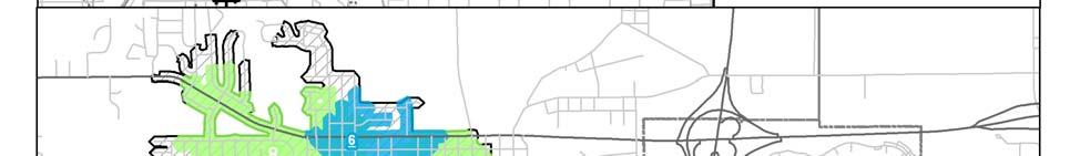
32 Figure 6. Cumulative K function, all rural crashes Ran Signal Ran Signal crashes are those caused by the failure to stop at locations with active traffic controls, specifically stop-and-go lights. This crash type was analyzed in part for the purpose of demonstrating the nature of the K function analysis. It was assumed that these crashes would experience a high degree of clustering because traffic signals are found, at specific points, almost exclusively in cities and some towns and generally only along highly traveled roads within these cities and towns. This expectation was confirmed by the graph in Figure 7. Crashes related to the running of traffic lights were by far the most clustered crash type analyzed. The bin-by-bin ratio values, as well as a moving average of these values, were used to identify scales at which signal running crashes appeared to be clustering more than crashes as a whole. Distances of 50, 150, 300, 500, and 1,700 meters were selected for polygon generation. The distances of 50, 150, 300, and 500 meters all had sharp increases in the ratio above expected values. The distance of 1,700 meters was selected to allow the capture of a general upward trend in the ratio between 1,300 and 1,700 meters. These values were then used as input parameters to identify locations and areas at the corresponding spatial scales of analysis. The number of excess crashes was used to identify and rank the hot spots at the various spatial scales, as explained above. The results are shown on Figure 8. 18

33 Figure 7. Ran Signal crashes vs. all crashes K function comparisons As distances increase above 2 or 3 kilometers, the fluctuations in the ratio can be attributed almost entirely to first-order effects, and in fact they probably serve as a good guide to the degree to which first-order effects impact other crash types. The ratio increases again around 9,000 meters (not shown on graph) when the Cedar Falls-Waterloo intercity clustering gets picked up. Beyond 10,000 meters, the ratio for Ran Signal crashes falls off drastically, reflecting the fact fewer signals are present outside city limits. The variation in ratios from one 50 meter bin to the next is extreme. At distances less than 50 meters, Ran Signal crashes are over 14 times more likely to occur than crashes in general (All Crashes). Yet when the bin distance is extended to instead capture crashes between 50 and 100 meters apart, the ratio is only 2 to 1. This may be because the distance range of the bin is too large to capture crashes at a single intersection yet not large enough to pick up crash pairs occurring at two separate intersections, i.e., traffic signals are farther apart than 100 meters. (This up-and-down pattern of the values is similar to tests performed earlier in this project in which an even grid of crashes was produced to see how the resulting K function performed in different circumstances.) 19

34 Figure 8. Ran Signal crash hot spots 20

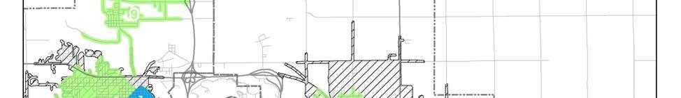
35 Polygons were generated for the various distances, and calculations were made for the excess crashes occurring within each polygon (Figure 8). While not entirely surprising, the results reveal that the best opportunity to reduce Ran Signal crashes is at the busiest intersections, specifically those at the intersections of major urban roads in and near downtown areas. On such roads, the higher levels of traffic and speed mean that failing to see a stop signal has a much greater likelihood of producing a crash. Possible remedies include those typically considered for intersections where red light running occurs (e.g., signalization, warning signs, and potentially red light running cameras). Interestingly, some of the larger polygons, using the 1,700 meter distance, do not have smaller hot spot polygons within them, indicating potential area-wide problems even if few, if any, intersections or adjacent sets of intersections appear to be particularly problematic. Examples include the area in southwest Cedar Falls, a largely residential area west of downtown Waterloo; Highway 58 north of US 20; and Highway 63 north of Highway 20. This illustrates the potential usefulness of considering the clustering of crash types at multiple scales. Distracted Driving Based on the clustering ratio (i.e., the ratio of distracted driver crashes to all crashes) consistently being above zero at the smaller distances, Figure 9 suggests that Distracted Driver crashes are an urban-dominated phenomenon. This is based on the fairly significant and consistent rate reduction beyond the 15 kilometer mark, which was denoted earlier as the extent of the Cedar Falls-Waterloo influence. This pattern is confirmed by the hot spot map generated (Figure 10). The map, however, reveals that such crashes are not limited to Waterloo and Cedar Falls, but are also seen significantly in the smaller outlying cities and towns. The most noticeable aspect of Figure 9 is the sudden peak at 200 meters before the bin-by-bin curve immediately returns to more normal values. In Cedar Falls and Waterloo, most standard near-square city blocks were measured to be between 90 and 125 meters per side. Waterloo, however, also has a significant number of rectangle blocks that tend to measure roughly 160 to 210 meters on the longer axis. If distracted driving were purely an intersection problem, the 100 to 150 meter range might also have a significantly higher ratio, but that is not the case; the ratio indicates only a slight degree of clustering. 21

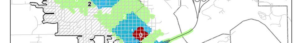
36 Figure 9. Distracted Driver crashes vs. all crashes K function comparisons In Figure 10, the highest ranked hot spots occur at a variety of locations within populated areas. The top ten 200 meter hot spots occur along frontage roads, along downtown area arterial routes, in purely residential areas, and in areas with no road classes above local streets. While this analysis is able to identify several locations of concern, there are few identifiable underlying factors. Crash report narratives, and perhaps site visits, might help to detect the nature of any distracting features or situations (e.g., visual clutter, landscape features, traffic, road geometry, intersections) or whether the hot spots are truly random occurrences. Distracted driver problems are often linked to in-car activities (cell phones, radios, eating and drinking), but they seem to interact with the roadway or geographic environment in some way because the consequences are felt in specific places. Distracted Driver crashes in this study area are very much an urban problem. Even at the larger distances shown in Figure 10, nearly all hot spot polygons were centered on cities and towns. Remedies would include both reviews of identified sites, to make the roadway environment less distracting or more forgiving, as well as more general policies regarding distracting activities, e.g., using cell phones while driving. 22

37 Figure 10. Distracted Driver crash hot spots 23

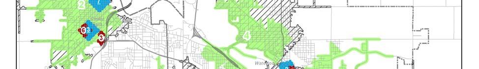
38 Older Drivers Older drivers, for the purposes of this analysis, are defined as those aged 65 and above. When the K function was performed, there were few obvious distances at which Older Driver crashes significantly clustered relative to All Crashes (Figure 11). There were general increases in the clustering ratio at distances around 5 kilometers and 34 kilometers. The increase at 34 kilometers (not shown on Figure 11) is likely a first-order effect because the concentration of Older Driver crashes in the Cedar Falls-Waterloo area began clustering with some of the more populated surrounding cities such as Waverly and Independence. The hot spots at the 34 kilometer scale were not mapped because the resulting hot spot polygons would have been excessively large and not helpful in aiding the search for specific locations in which targeted countermeasures could be applied. Instead, the minor spikes in the Older Driver ratio at distances less than 5 kilometers were focused on. Using Figure 11, the distances of 550 meters, 3,850 meters and 4,900 meters were selected for closer analysis. Figure 11. Older Driver crashes vs. all crashes K function comparisons The identification of hot spots (Figure 12) at the three scales reveals the areas where most excess crashes occur, namely within cities and towns of at least 1,000 residents. Using the smallest (550 meter) distance within the cities, the problem appears quite focused. There is a concentrated area within Waterloo in which four of the top ten hot spots appear, including three of the top five hot spots This concentration occurs near a big-box shopping district lined with a mall, fast food 24

39 restaurants, and home improvement, home electronics, grocery, and office supply stores. In this area, Older Driver crashes are nearly double the expected value. A hot spot in a big-box shopping district between Cedar Falls and Waterloo (colloquially referred to as Cedarloo) also appears as a hot spot. Slightly less severe but still a significant problem are downtown areas. Such locations have several variables possibly contributing to Older Driver crashes. These locations generally feature two or more lanes in each direction of travel, as well as many turn lanes. There are frequent stop-and-go lights despite posted speeds of 30 or more miles per hour. In the shopping areas, turn lanes, frontage roads, and many business entrances contribute to creating an environment with a great deal of activity and potentially confusing situations. In downtown areas identified with hot spots (Cedar Falls, Waterloo, Independence, and New Hampton), similar situations of potentially confusing roadways and a great deal of turning traffic also occur. The number of crashes in these locations suggests older drivers are especially unprepared to meet the unique challenges presented at such locations. Possible countermeasures include taking further steps to simplify traffic flow in these areas. Besides modifying the roadway, the involvement of a very clear demographic influence means that trying to reduce the factors is a possible option through programs specifically designed for older risk via human drivers. 25

40 Figure 12. Older Driver crash hot spots 26

41 Younger Drivers Younger drivers are defined as those aged 14 through 24. Iowa residents are eligible to receive their Instruction Permit at age 14. Individuals at that age are widely accepted as being the most dangerous demographic group of drivers. It was thought that performing a study on the spatial characteristics of their crashes might reveal specific locations and situations in which younger drivers struggle to respond appropriately when behind the wheel. Figure 13 reveals a peak in clustering after approximately 14 kilometers, and a drop off in clustering thereafter. This trend was interpreted initially as indicating that Younger Driver crashes are typically more urban than rural. This distance was not used to generate hot spots because of the computational requirements necessary given the network distances and number of crashes involved, as well as expected issues in interpreting hot spots using such a distance. Figure 13. Younger Driver crashes vs. all crashes K function comparisons At a more local level, several peaks were investigated using distances of 200 meters, 550 meters, 850 meters, and 1,650 meters (Figure 14). Not surprisingly, the locations of several hot spots are associated with educational institutions, in particular the University of Northern Iowa (UNI), where driving exposure rates for younger drivers are high. Additional educational facilities with their own distinct hot spots include Wartburg College (Waverly), Hawkeye Community College (Waterloo), and West High School (Waterloo). 27

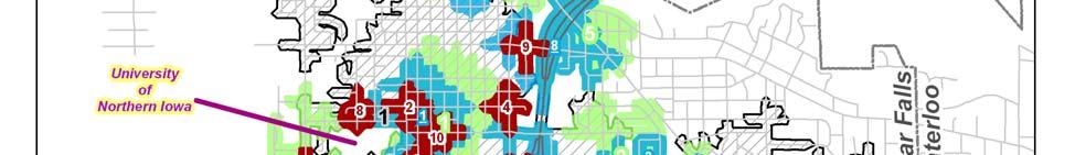
42 Figure 14. Younger Driver crash hot spots 28

43 Younger Driver crashes also appear to cluster in certain areas, specifically areas with entertainment, shopping, and employment (e.g., College Square Mall, downtown Cedar Falls), and major road segments to and from these areas. Younger Driver hot spot locations seem heavily influenced by the travel patterns of students between their places of learning and residence and their places of entertainment and shopping. Several of these hot spots seem to reflect problems with intersections, turning traffic, and business entrances. Based on these results, countermeasures to address Younger Driver crashes might include enforcement, education (especially with respect to novice drivers and complex driving situations), and efforts linked to younger driver travel patterns. Further analysis could focus on driver actions and the contributing circumstances of crashes within each hot spot. Local Roads For this study, local roads were identified by means of the definition used in the Iowa Comprehensive Highway Safety Plan (CHSP) (Iowa DOT 2007), a document that guided the determination of which crash types to include in this report. The Iowa CHSP states that local roads are those under the jurisdiction of Iowa s 99 counties and 947 cities. (An alternative definition would have been FHWA s functional class, which defines roads more by their purpose.) This includes a majority of miles of Iowa roads, as well as a majority of crashes in the study area. The result was the creation of a crash type with the highest number of crashes (13,502) in the study. Local Road crashes exhibited positive clustering ratios for nearly the entire span of distances up to 20 kilometers. The most significant and consistent clustering, however, occurred at distances under 5 kilometers (Figure 15). Due to the varying nature of the ratio under 5 kilometers, polygons were generated to examine hot spots at distances of 300 meters, 500 meters, 2,650 meters, and 3,550 meters. 29

44 Figure 15. Local Road crashes vs. all crashes K function comparisons Mapping out the hot spots at these scales revealed (Figure 16), not surprisingly, that the greatest number of excess crashes occurs within Cedar Falls and Waterloo. Likely as a result of the definition used, which includes arterial and collector roads under the jurisdiction of the cities as local roads, the hot spots are centered on the intersections of major routes. With such a generalized crash type, the hot spots reveal little more than that most excess crashes occur where there are high traffic volume roads meeting. 30

45 Figure 16. Local Road crash hot spots 31

46 To better understand Local Road crashes, the entire process was repeated excluding crashes within city limits (Figure 17). This rural-only perspective was completed with the expectation of revealing dangerous roads in rural areas that may not have shown up in Figure 16 simply because of lower traffic volumes. The spikes at distances of 50 meters and 1,050 meters were selected for further analysis. Similar to the analysis that included urban areas, the rural-only hot spot analysis (Figure 18) showed that the problem areas are where collector or higher functional class roads intersect. (There were few enough crashes occurring in the hot spots to cause several exact ties in the excess crashes value, as shown on the map.) Of particular interest for this study area are the multiple hot spots along County Road C-57, also known as Cedar-Wapsi Road, which runs eastwest to the north of Waterloo. Nearly every intersection of this minor collector road with other collector level roads makes the top ten hot spots list. The crash history of these intersections suggests that targeted roadway improvements at these locations may be beneficial, such as flashing red lights mounted on stop signs, or rumble strips if it is a matter of drivers not noticing the stop signs. Some of the crashes may be a result of drivers misjudging the rate of speed at which cars on the perpendicular route are approaching. A closer analysis of the cause of the crashes at these intersections may reveal which action is appropriate at each particular intersection. Figure 17. Local Road crashes vs. all crashes K function comparisons (rural only) 32

47 Figure 18. Local Road crash hot spots (rural only) 33

48 Lane Departure Several fields in the Iowa DOT crash database suggest a departure from the proper lane of travel. The definition used in this study is based on the MajorCause field of the database. Four such possible causes were included: (1) crossed centerline, (2) run off road right, (3) run off road straight, and (4) run off road left. Figure 19 reveals a very distinctive clustering ratio line for Lane Departure crashes. This type of crash was underrepresented at distances up to 16 kilometers, the range normally associated with urban crash patterning. With no clustering at shorter distances, and the inability to gather much information from a map of hot spots at extremely large distances (covering large portions of a county), no hot spot map was created to correspond to Figure 19. Figure 19. Lane Departure crashes vs. all crashes K function comparisons However, based on Figure 19, the clustering appears to be mainly a rural problem, so an identical K function operation was run on Lane Departure crashes falling outside city limits. The resulting graph can be seen in Figure 20. Once again, very few distances cross into a positive ratio value, suggesting minimal clustering that is possibly as much a result of random variations than any real trend. Nonetheless, a hot spot map (Figure 21) was generated for several of the most clustered distances. 34

49 Figure 20. Lane Departure crashes vs. all crashes K function comparisons (rural only) In Figure 21, there are 16 polygons representing the 50 meter scale. Each 50 meter hot spot labeled with a rank of 1 has merely three excess crashes. There may indeed be problems with those particular locations; however, the nature of the problem is not immediately clear from looking at the map. All other 50 meter polygons have two or fewer excess crashes, making it difficult to suggest that there are truly problems at these locations rather than simply random fluctuations. In this case, mass action remedies may be more effective than spot improvements of weak hot spots. At a broader spatial scale, the 2,500 meter and 5,300 meter polygons are large enough to encompass enough crashes to be more certain of the overrepresentation of Lane Departure crashes. Most of these larger hot spots are centered on arterial and collector functional class roadways. The fact that these crashes occur on what are mainly paved roads means that fairly simple improvements, such as more visible white lines, wider shoulders, or shoulder rumble strips may provide fairly low-cost yet highly effective results in these problematic areas. Specific problematic roads in this study area include US 218 between Janesville and Waverly, and County D-48/Brandon Road, located northeast of La Porte City. 35

50 Figure 21. Lane Departure crash hot spots (rural only) 36

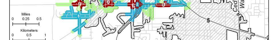
51 Impaired Driving For this study, impaired driving included only improper alcohol consumption. The use of illegal drugs, or the improper use or overdose of medical drugs, was not included. Only crashes involving a driver with a blood alcohol content over 0.08 were included in the dataset analyzed. The ratio line in Figure 22 fluctuates up and down along the zero line, but never rises above 0.75 (until the distance scale is large enough to make mapping the hot spots fairly meaningless). Such a pattern of ratios reflects the existence of little if any real clustering at any spatial scale. A map was generated (Figure 23) at scales of 2,000 meters and 5,000 meters. In both situations, the ratio is near zero (meaning the crash clustering rate is no more or less than the expected value). These sizes were chosen because they typify the line as a whole and could possibly reveal where Impaired Driving crashes generally occur. While Figure 23 displays hot spots, few are truly hot. Using the 2,000 meter polygons, only two hot spots were identified as having an excess, one excess crash in each. The 5,000 meter hot spots were more successful at identifying problematic areas. By far, the worst single hot spot identified, containing over 30 excess crashes, corresponded to the areas connecting the University of Northern Iowa with downtown Cedar Falls and the University of Northern Iowa with Cedarloo along University Avenue. The presence of bars in both areas popular with students at UNI raised suspicions that students may be the cause for that particular hot spot. To test this hypothesis, the driver age was joined to the crash data. Out of the 106 impaired drivers involved in crashes found within this hot spot, 65 were less than 25 years old, and 28 drivers were under 21 years old. A free shuttle service from the campus area to several of the bars in question already exists, leaving education and stricter enforcement as the logical course of action to reduce crashes in that particular hot spot. Why the hot spot southeast of Waterloo exists is not clear. The rest of the hot spots contain fairly insignificant numbers of excess crashes, five or fewer in each, reflecting the weak clustering values seen throughout Figure

52 Figure 22. Impaired Driver crashes vs. all crashes K function comparisons 38

53 Figure 23. Impaired Driver crash hot spots 39

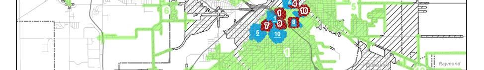
54 Failure to Yield Right of Way Failure to Yield Right-of-Way (FTYROW) crashes are typically thought of as occurring at intersections, and most do. There are, however, other situations in which these crashes can occur. This study used all crashes with the following FTYROW designations, as identified in the Iowa DOT crash database: At uncontrolled intersection Making right turn on red From stop sign From yield sign Making left turn From driveway From parked position To pedestrian Other Because most of these crashes are expected to be intersection-based, it was anticipated that the strongest clustering would occur at smaller scales. This expectation is supported by Figure 24. (Increases at 10 kilometer and 15 kilometer distances, not shown, also occurred, likely as a result of first-order effects.) The spikes in the ratio at smaller scales were mapped to produce hot spots, the results of which are shown in Figure 25. The distances mapped are 100 meters, 450 meters, and 650 meters, all of which reached a ratio value above 1 (i.e., twice the rate expected of the crash type). The 100 meter hot spot polygons highlight issues at specific intersections. As logically expected, more excess crashes occurred at intersections on highly traveled arterial roadways, particularly where lined with businesses, meaning there were high levels of traffic making turns. Once again, the mall and big-box shopping districts in southeastern Waterloo and the Cedarloo area, between Cedar Falls and Waterloo, are among the worst areas. The fact that this characteristic is shared with both the Older Driver crashes and Younger Driver crashes suggests a correspondence between these demographic groups and FTYROW crashes in these locations. The larger hot spot polygons, 450 meters and 650 meters, also picked up the same problem areas but also added new areas. Interestingly, these polygons did not highlight downtowns, but rather residential areas just beyond downtowns. These areas of dense residential neighborhoods, southwest of downtown Cedar Falls, south of Waterloo s downtown, and just northeast of the University of Northern Iowa campus (see Figure 14 for the location of the campus), all appeared as hot spots. There are a number of possible contributing factors to this, including (1) the highdensity road network, (2) minimal traffic controls in most situations, (3) insufficient sight lines at intersections caused by dense on-street parking, and (4) drivers disregarding traffic control signs due to familiarity with the neighborhood in which they live. The appearance of different hot spots at different scales, highlighting potentially different problems and countermeasures, illustrates the importance of scale when analyzing crash patterns. 40

55 Figure 24. Failure to Yield Right-of-Way crashes vs. all crashes K function comparisons 41

56 Figure 25. Failure to Yield Right-of-Way crashes hot spots 42

57 Fatal and Major Injury Fatal and Major Injury crashes were combined in this study. Initially, an analysis was conducted solely on fatal crashes; however, given the relatively low number of crashes involved and their dispersed spatial distribution, the results were idiosyncratic. (The clustering ratio sharply increased and decreased in response to specific pairs of crashes being within certain distances of each other, and hot spots had few crashes and typically were not meaningful.) Instead, crashes involving fatalities or major injuries were used to analyze the spatial distribution of severe crashes (i.e., those that resulted in a fatality or narrowly avoided it). The resulting ratios shown in Figure 26 were consistently below zero, meaning that fatal and near-fatal crashes did not cluster and were actually dispersed beyond what was expected. There were, however, areas in which the ratio was closer to zero than on average. To investigate this, a hot spot map was produced (Figure 27) of the 50 meter distance bin. Figure 26. Combined Fatal and Major Injury crashes vs. all crashes K function comparisons 43

58 Figure 27. Combined Fatal and Major Injury crash hot spots 44

59 The majority of the hot spots identified at the 50 meter scale appeared where arterial or collector roads intersected one another. Most hot spots also occurred either outside cities or on roads within cities that allowed travel at 45 miles per hour or more. Those hot spots occurring outside the city often occurred at intersections where one route is given right of way and is allowed to continue at highway speeds while the other route must stop and then proceed across or onto the perpendicular route. When two high-traffic roads are involved, this situation results in a significant amount of crossing or merging traffic and exposure to possible side impact crashes with one of the vehicles traveling at a high rate of speed. Possible solutions vary depending on the road configuration. The top-ranked hot spot is at a location where traffic from County Road C-57/Cedar-Wapsi Road must, from a stop, either merge or cross traffic traveling at 65 miles per hour. One countermeasure would be to upgrade the intersection. Some hot spots, however, already have similar measures in place; hot spot number three has stop-and-go lights installed, and hot spot number six has dedicated on- and off-ramps. To further explore the issue of fatalities, a rural-only crash database was produced of fatal and major injury crashes falling outside city limits. The resulting graph can be seen in Figure 28. With the influence of urban areas removed, fatal and major injury crashes experienced an increase in clustering ratios. Three clear peaks appeared at distances of 50 meters, 1,800 meters, and 5,050 meters. The 50 meter distance could be explained by several fatal or major injury crashes occurring at the same intersections, but the other spikes did not offer any obvious explanations. Mapping the rural-only hot spots generated interesting results, as seen in Figure 29. Most of the top 50 meter hot spots seen in Figure 27 remained. While the locations experienced little change, it was the numbers behind the hot spots that show the clear differentiation. Within the hot spots for fatal and major injury crashes in general (urban areas included), there was a fatality or major injury in 14% of crashes. The same statistic for rural-only hot spots is 35% of crashes. Crashes in these rural hot spots were less common, but when they did happen, the odds of a fatality or major injury was significantly higher. In seven of the top ten rural hot spots, a fatality or major injury was experienced in 50% or more of crashes occurring there. These hot spots are extremely critical areas within the INRCOG region. The aforementioned interchange between US 218 and C-57/Cedar-Wapsi Road experienced five fatal or major injury crashes in the five years of data explored, or one serious crash per year. If that intersection were to be simply as safe as the average intersection within INRCOG, it would be expected to experience a fatal or major injury crash once every 3.6 years. In the rural-only analysis, larger polygons were also generated for meter and 5,050 meter distances. The 5,050 meter polygons were too large to allow meaningful information to be gathered from them. The 1,800 meter hot spot sizes, however, did prove useful. Many of them corresponded to the locations of the 50 meter hot spot polygons, revealing the importance of these locations in terms of fatal or major injury crashes. There also were several new locations highlighted, revealing areas in which such crashes are significant not at a particular intersection, but along a particular short stretch of road, or revealing a combination of a problematic intersection and crashes along the roadway leading up to that intersection. While these crash hot spot locations could be revealed by the analysis, their causes are not immediately identifiable. A further analysis of the contributing circumstances of each crash within the hot spots, or an on-site inspection, may reveal further clues in these situations. 45

60 Figure 28. Combined Fatal and Major Injury crashes vs. all crashes K function comparisons (rural only) 46

61 Figure 29. Combined Fatal and Major Injury crash hot spots (rural only) 47

62 Speeding Many drivers often exceed the posted speed limit, and speeding likely contributes to many crashes. For the purpose of this analysis, however, the interest was in crashes for which speeding was the primary factor. These were identified by using crashes for which the Iowa DOT crash database recorded excessive speed as the major cause. Figure 30 shows a graph quite different from most others produced in this study. The ratios indicate that speeding-related crashes experienced some of the strongest clustering of all crash types reviewed in this study. The ratio also has a general increasing trend up to a distance of roughly 4,000 meters. The relatively low number of Speeding crashes (193), however, does raise some concerns about the significance of the findings. The graph indicates a fair amount of variation from bin to bin, but the overall trend with increasing distance remains clear. Figure 30. Speeding crashes vs. all crashes K function comparisons Three scales of hot spots were mapped in Figure 31. At the 4,200 meter scale, only seven of the polygons generated contained an excess number of Speeding crashes, of which only the top two (Waterloo and Evansdale) can be considered hot spots of any significance. The 200 meter and 1,300 meter hot spots are almost entirely centered on the city of Waterloo. Most of these hot spots were found within residential neighborhoods. A closer inspection of the specific crash 48

63 locations showed that within these hot spots, the problem is often not on arterial or even collector streets, but on local streets within the neighborhoods. A possible cause for hot spots occurring at these locations, a feature relatively unique among the crash types analyzed, is the greater overall road environment. Arterial and collector roads are often engineered with wide lanes, generous shoulders, and limited or no on-street parking, which may make these routes relatively forgiving to individuals who choose to speed. These same characteristics are often not found on local streets, especially those in neighborhoods built before modern roadway safety engineering. Dense residential neighborhoods with many people, intersections, driveways, and on-street parking create many hazards. As such, a solution that might hold the most promise toward reducing this crash type is stricter enforcement of speed limits in these residential areas. 49

64 Figure 31. Speeding crash hot spots 50