ECE 102 Engineering Computation

Size: px

Start display at page:

Download "ECE 102 Engineering Computation"

Jeffery Houston
5 years ago
Views:

1 ECE 102 Engineering Computation Phillip Wong MATLAB XY Plots with Linear-Linear Scaling Formatting Plots XY Plots with Logarithmic Scaling Multiple Plots Printing and Saving Plots

2 Introduction to 2D Graphs MATLAB supports 2D and 3D graphs for visualizing data sets. Available 2D graph types include: XY Scatter Stem Line Pie Histogram Bar Polar Contour There are extensive options for customizing the appearance of a graph. 1

3 XY Plots with Linear-Linear Scaling Linear XY plots: plot(x,y) The axes are linear in both xand y. xand yare vectors of the same length. x contains the independent data values. y contains the dependent data values. The plot appears in the Figure Window. 2

4 Enhanced plot command: plot(x,y,'propertyname',value) -orplot(x,y,'specifiers') PropertyName, Value set individual line and marker properties (e.g., style, color). Specifiersquickly define line and marker properties in a single string. XY plot with primary and secondary Y axes: plotyy(x1,y1,x2,y2) 3

5 Line Property Names: LineStyle LineWidth Color Value Description Color 'b' 'r' blue (default) red Style Value '-' '--' ':' '-.' 'none' Description solid (default) dashed dotted dash-dot no line 'g' 'c' 'm' 'y' 'k' 'w' green cyan magenta yellow black white Width Value Description 1 thinnest (default) 2 to 100 thicker line [R,G,B] R = Red (0 to 1) G = Green (0 to 1) B = Blue (0 to 1) 4

6 Marker Property Names: Marker MarkerSize MarkerEdgeColor MarkerFaceColor Marker size is an integer starting at 1. Marker color values are the same as the line color values. Marker Value '+' 'o' '*' '.' 'x' 's' 'd' '^' 'v' '>' '<' 'p' 'h' Description plus sign circle asterisk point cross square diamond triangle-up triangle-down triangle-right triangle-left 5-point star 6-point star 5

7 Example: x = -2*pi:pi/24:2*pi; y = sinc(x); plot(x,y) Blue solid line, no markers plot(x,y,'linestyle',':','color','r') Red dotted line, no markers plot(x,y,':r') Red dotted line, no markers plot(x,y,'om') plot(x,y,'-sk') No line, magenta circle markers Black solid line, black square markers 6

8 plot(x,y) plot(x,y,'linestyle',':','color','r') -orplot(x,y,':r') 7

9 plot(x,y,'om') plot(x,y,'-sk') 8

10 Formatting Plots Clear Figure clf Erases the Figure window New Figure figure(n) Opens a new figure window (index n) (optional if only one figure needed) Axis Grid Lines grid on Adds major grid lines grid minor Toggles minor grid lines grid off Removes all grid lines 9

11 Axis Limits axis([xmin xmax ymin ymax]) xmin xmax ymaxorymin yminorymax Note: Limits are specified in a vector. All four limits must be present. If a particular limit is specified as +inf or inf, then its value is autoset. Variations: axis auto axis xy axis ij Sets both axes limits automatically Sets origin to lower left corner Sets origin to upper left corner 10

12 Axis Labels xlabel('x axis text string') ylabel('y axis text string') Title title('one line text string') title({'two lines', 'of text'}) brace comma Text Box text(xpos,ypos,'text string') brace Note: xposand yposare coordinates relative to the graph s origin where the text should appear. 11

13 Greek characters and subscripts/superscripts can be displayed in text by embedding special sequences in the string. Symbol Sequence Symbol Sequence Symbol Sequence α \alpha ρ \rho ϒ \Upsilon β \beta σ \sigma Φ \Phi γ \gamma τ \tau Ψ \Psi δ \delta υ \upsilon Ω \Omega ɛ \epsilon φ \phi ζ \zeta χ \chi η \eta ψ \psi θ \theta ω \omega ι \iota Γ \Gamma κ \kappa Δ \Delta λ \lambda Θ \Theta µ \mu Λ \Lambda ν \nu Ξ \Xi ξ \xi Π \Pi Subscript _{text} π \pi Σ \Sigma Superscript ^{text} 12

14 Text Font Property Names: FontName FontSize FontAngle FontWeight Name Value Description Angle Value Description 'Helvetica' 'Times' 'Courier' 'FixedWidth' Helvetica font Times font Courier font Localized fixed font 'normal' 'italic' 'oblique' normal (default) slanted font slanted font Size Value Description 1 to 128 font point size Weight Value 'normal' 'demi' 'bold' Description normal (default) bold font bold font 13

$1]) title('graph of y = 2exp(-\alpha_{0}^{2})',... 'FontName', 'Helvetica', 'FontSize', 14) xlabel('position \alpha_{0} (mm)', 'FontWeight', 'Bold') ylabel('intensity I_g (mw/mm^2)') text(0.$

15 Example: Plot 2 α 0 = e where 20 α 0 5 I g 2 Before formatting % Initialize data alpha_0 = -20:0.1:5; Ig = 2 * exp(-alpha_0.^2); % Basic plot clf plot(alpha_0, Ig) % Formatting axis([ ]) title('graph of y = 2exp(-\alpha_{0}^{2})',... 'FontName', 'Helvetica', 'FontSize', 14) xlabel('position \alpha_{0} (mm)', 'FontWeight', 'Bold') ylabel('intensity I_g (mw/mm^2)') text(0.3, 2, 'Peak value') 14

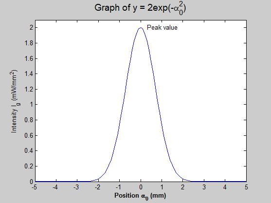
16 After formatting 15

17 XY Plots with Logarithmic Scaling XY plots with at least one log scale: semilogx(x,y) semilogy(x,y) loglog(x,y) log x, linear y linear x, log y log x, log y xand yare vectors of the same length. x contains the independent data values. y contains the dependent data values. 16

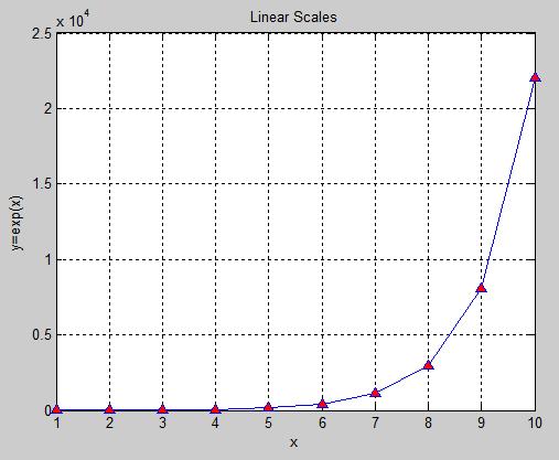
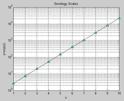
18 Example: Plot y = e x for 0 x 10. Try different scales. x = 1:10; y = exp(x); figure(1) plot(x,y,'-^','markerfacecolor','red'); grid on xlabel('x'); ylabel('y=exp(x)'); title('linear Scales') figure(2) semilogy(x,y,'-^','markerfacecolor','green'); grid on xlabel('x'); ylabel('y=exp(x)'); title('semilogy Scales') 17

19 18

20 Multiple Lines in the Same Plot Method #1: plot command plot(x1,y1,'spec',x2,y2,'spec', ) All the lines are overlaid on the same plot. Each line can have its own specifiers. 19

21 Adding a Legend legend('str1','str2', ) Variations: legend('str','location', Loc_Value) Loc_Value is a predefined value that puts the legend at a specific location on the plot. legend('off') legend('show') legend('boxoff') legend('boxon') Turn off legend Show legend Remove box from legend Add box around legend 20

22 Allowed legend location values: Location Value Description Location Value Description 'North' Inside top 'EastOutside' Outside right 'South' Inside bottom 'WestOutside' Outside left 'East' Inside right 'NorthEastOutside' Outside top right 'West' Inside left 'NorthWestOutside' Outside top left 'NorthEast' Inside top right 'SouthEastOutside' Outside bottom right 'NorthWest' Inside top left 'SouthWestOutside' Outside bottom left 'SouthEast' Inside bottom right 'Best' Least conflict 'SouthWest' Inside bottom left 'BestOutside' Least unused space 'NorthOutside' Outside top 'SouthOutside' Outside bottom 21

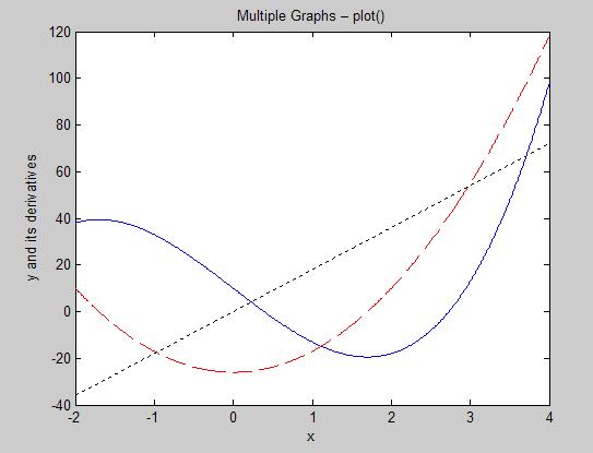
23 Example: Plot y 1 = 3x 3-26x + 10, y 2 = 9x 2-26, and y 3 = 18x over the interval-2 x 4. x = -2:0.01:4; y1 = 3*x.^3-26*x+10; y2 = 9*x.^2-26; y3 = 18*x; plot(x,y1,'-b', x,y2,'--r', x,y3,':k') xlabel('x') ylabel('y and its derivatives') title('multiple Graphs plot()') 22

24 23

25 Method #2: hold command hold on Each new plot command adds a graph that is overlaid on the current graph (Place this after the first plot command) hold off Turns off hold mode, so each plot command creates a new graph 24

26 Example: Plot sin(2πt) and cos(2πt) on the same graph over the interval -π t +π. t = -pi:0.01:pi; y1 = sin(2*pi*t); y2 = cos(2*pi*t); plot(t,y1,'r') axis([-pi pi ]) hold on plot(t,y2,':b') title('multiple Graphs - hold') xlabel('time (seconds)') ylabel('amplitude (Volts)') legend('sin','cos','location','northeastoutside') hold off 25

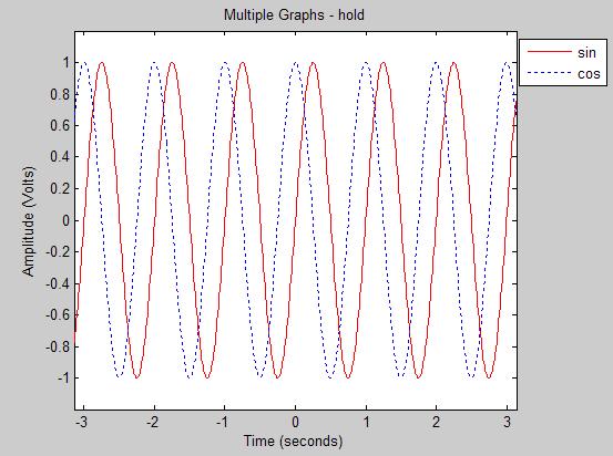
27 26

28 Example: VD = 0.6:0.005:0.8; % V : Applied diode voltage k = e-23; % J/K : Boltzmann's constant q = e-19; % C : Electric charge IS = 1.0e-12; % A : Reverse saturation current I1 = IS * (exp(vd / (k*250/q)) - 1); % A : Diode T = 250 K I2 = IS * (exp(vd / (k*255/q)) - 1); % A : Diode T = 255 K I3 = IS * (exp(vd / (k*260/q)) - 1); % A : Diode T = 260 K clf grid on plot(vd,i1,'r','linewidth',2) axis([ e3]) hold on plot(vd,i2,'--m','linewidth',2) plot(vd,i3,':b','linewidth',2) xlabel('applied diode voltage V_{D} (V)','FontSize',12) ylabel('diode current I_{D} (A)','FontSize',12) title({'dependence of diode current on temperature T',... 'Parameters: I_{S} = 1 pa, Ideality factor \eta = 1'},... 'FontSize',14) legend('t=250 K','T=255 K','T=260K','Location','Best') hold off I( V D ) = I S e V D kt q 1 27

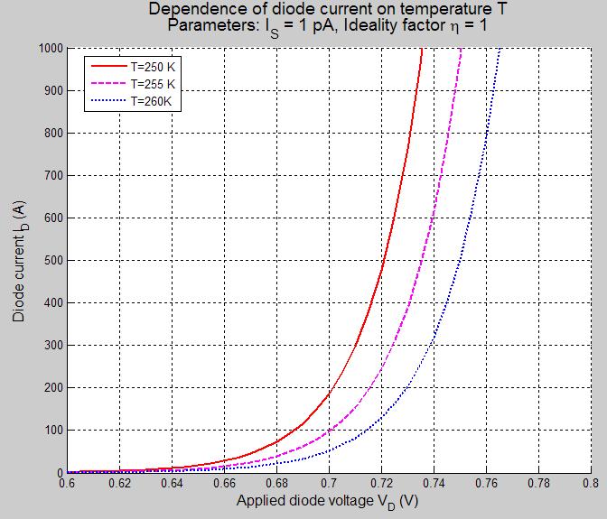
29 28

30 Method #3: line command line(x,y,'propertyname',value) Adds an additional line to a pre-existing plot. 29

31 Example: Plot y 1 = x, y 2 = x 2, and y 3 = x 3 over -2 x 2. x = -2:0.01:2; y1 = x; y2 = x.^2; y3 = x.^3; plot(x,y1,'linestyle','-','color','r','linewidth',1) line(x,y2,'linestyle','--','color','c','linewidth',2) line(x,y3,'linestyle',':','color','m','linewidth',3) xlabel('x'); ylabel('powers of y') title('multiple Graphs line()') 30

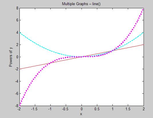
32 31

33 Multiple Plots on the Same Page subplot command subplot(m,n,k) Places the plot as a tile at position kon an m ngrid Example: 2 2 grid: (2,2,1) (2,2,2) (2,2,3) (2,2,4) 2 3 grid: (2,3,1) (2,3,2) (2,3,3) (2,3,4) (2,3,5) (2,3,6) 32

34 Example: Plot y 1 = x 2 and y 2 = x sin(4x) as 1 2 tiled graphs over the interval 0 x 10. x = 0:0.1:10; y1 = x.^2; y2 = x.*sin(4*x); subplot(1,2,1); plot(x,y1,'--') xlabel('x'); ylabel('y1=x^2') title('tile 1 subplot(1,2,1)') subplot(1,2,2); plot(x,y2,':') xlabel('x'); ylabel('y2=xsin(4x)') title('tile 2 subplot(1,2,2)') 33

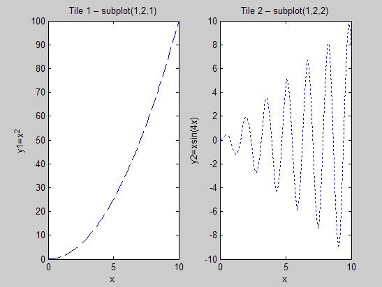
35 34

36 Printing and Saving Plots To send the current plot to the printer: print To save the current plot to an image file: print dtype filename type = ps, psc, eps, epsc, tiff, jpeg, png Example: print djpeg myplot Image files are saved to the current directory. 35

COMP MATLAB.

COMP MATLAB. COMP1131 MATLAB chenyang@fudan.edu.cn 1 2 (x, y ) [(x 1,y 1 ) (x 2,y 2 ) (x n,y n )] Y=f(X) X [x 1,x 2,...,x n ] Y [y 1,y 2,,y n ] 3 MATLAB 4 figure figure figure(n): n figure(n) 5 y = x + sin x (x [ π