Master of Spatial Analysis

Transcription

1 Predicting the Contamination between Sites of Sediment Core Measurement in Lake Ontario by Daniel J. Jakubek A Research Paper Presented to Ryerson University in partial fulfillment of the requirements for the degree of Master of Spatial Analysis A joint program with the University of Toronto Toronto, Ontario, Canada Daniel J. Jakubek 2002

2 Author s Declaration I hereby declare that I am the sole author of this Research Paper. I authorize Ryerson University to lend this Research Paper to other institutions or individuals for the purposes of scholarly research. Daniel J. Jakubek ii

3 Abstract Research activities involving the collection of sediment core samples are extremely time consuming and expensive to fund. This research utilized data from the Environment Canada Great Lakes Sediment Assessment Program. A total of 32 contaminants were measured at 70 sediment core-sampling locations in Lake Ontario. Various methods for the estimation of sediment contamination levels were investigated. The Sediment Quality Index (SQI) was calculated and assessed as being a satisfactory measure for areas where sediment quality is frequently threatened or impaired. Ordinary kriging was identified as the optimal spatial interpolation model. Individual prediction maps were successfully produced for 20 of the contaminants and crossvalidation was used to further assess 'ordinary kriging' as an appropriate method for predicting the spatial distribution of sediment contamination. The results rendered from cross-validation provided an assessment of the relative success of each of the interpolation procedures. Limitations including the limited number of sampling sites, and minimal data at Lake Ontario Areas of Concern, were the main factors for inaccurate prediction surfaces. iii

4 Acknowledgements I would like to express appreciation to my graduate faculty advisor Dr. Wayne Forsythe for his ongoing support and guidance while completing this research project, and throughout the Master of Spatial Analysis program. As a result of his assistance, personal goals set throughout the program were attainable. I would also like to thank Dr. Marie Truelove, Director of the M.S.A. program, whose organization enabled me to acquire professional experience at the Canadian Ministry of Environment through the practicum component of the program. While completing the required practicum with The Ecosystem Health Division, I was supplied with data that was utilized to perform the analysis in this research project. Sediment contamination levels were initially measured for use in the Environment Canada Great Lakes Sediment Assessment Program. Specifically, I would like to thank the following individuals for their support: Scott Painter, Watershed Scientist, Ecosystem Health Division, Canada Centre for Inland Waters, Canadian Ministry of the Environment Alice Dove, Watershed Scientist, Ecosystem Health Division, Canada Centre for Inland Waters, Canadian Ministry of the Environment iv

5 Table of Contents Author s Declaration ii Abstract iii Acknowledgements iv List of Tables vii List of Figures viii List of Acronyms xi Chapter 1: Introduction Introduction Pollution in the Great Lakes Study Area The Data Samples and Sampling Locations The Problem Sediment Contamination Research Objectives Chapter 2: Literature Review Sedimentation Processes in Lake Ontario Lake Ontario s Lakewide Management Plan Critical Pollutants and Sources of Loading in Lake Ontario Polychlorinated Biphenyls (PCBs) DDT and Its Metabolites Mirex Dioxins and Furans Mercury Dieldrin Application of the Sediment Quality Index in Lake Ontario Spatial Interpolation Kriging Ordinary Kriging Simple Kriging Universal Kriging Indicator Kriging Co-Kriging Probability Kriging Chapter 3: Methodology Calculation of the Sediment Quality Index (SQI) Spatial Interpolation: Deterministic Methods Inverse Distance Weighted Interpolation Radial Basis Functions v

6 3.2.3 Global Polynomial Interpolation Local Polynomial Interpolation Spatial Interpolation: Geostatistical Methods Regionalized Variable Theory (RVT) and Kriging Ordinary Kriging The Empirical Semivariogram Fitting a Model to the Empirical Semivariogram Anistrophy: Directional Influence of Autocorrelation Determining the Search Neighbourhood Cross-Validation: Identification of the Best Model Chapter 4: Results and Discussion Sediment Quality Index as a General Indicator of Sediment Contamination Deterministic Methods Inverse Distance Weighting Radial Basis Functions Global Polynomial Interpolation Local Polynomial Interpolation Geostatistical Methods Cross-Validation Results for Ordinary Kriging Limitations of the Data Sediment Quality Index Metals Critical Pollutants Polycyclic Aromatic Hydrocarbons (PAHs) The Remaining Contaminants Sampling Strategies Chapter 5: Summary and Conclusions References vi

7 List of Tables Table 1.1: Physical Characteristics of Lake Ontario 5 Table 1.2: Table of Contaminants and Federal Guidelines 11 Table 2.1: Origin of PCB Loadings to Lake Ontario 24 Table 2.2: Origin of DDT Loadings to Lake Ontario 25 Table 2.3: Origin of Mirex Loadings to Lake Ontario 25 Table 2.4: Origin of Dieldrin Loadings to Lake Ontario 27 Table 3.1: Deterministic Methods for Spatial Interpolation 39 Table 4.1: SQI and Critical Pollutants 61 Table 4.2: Results for Deterministic Methods of Spatial Interpolation 63 Table 4.3: Lake Ontario Sediment Contaminants: Semivariogram Models and Neighbourhood Search Size 72 Table 4.4: Cross-Validation Results for Ordinary Kriging 82 vii

8 List of Figures Figure 1.1: The Golden Horseshoe 1 Figure 1.2: The Great Lakes Basin 2 Figure 1.3: Lake Ontario Bathymetry 6 Figure 1.4: Lake Ontario Drainage Basin 7 Figure 1.5: Lake Ontario Sediment Sampling Locations 9 Figure 2.1: Lake Ontario Sedimentary Basins 16 Figure 2.2: Annual Current Circulation Patterns in Lake Ontario 18 Figure 3.1: Exponential Model Fitted to SQI Measurements 50 Figure 3.2: Predicted Values Vs. Measured Values 56 Figure 3.3: Error Plot 56 Figure 3.4: Standard Error Plot 57 Figure 3.5: QQ Plot 57 Figure 4.1: Lake Ontario Contaminated Sediment Stations 60 Figure 4.2: Inverse Distance Weighting SQI Scores 65 Figure 4.3: Radial Basis Functions SQI Scores 66 Figure 4.4: Global Polynomial Interpolation SQI Scores 67 Figure 4.5: Local Polynomial Interpolation SQI Scores 68 Figure 4.6: Ordinary Kriging SQI Scores 77 Figure 4.7: Deterministic Interpolations Vs. Kriging 80 Figure 4.8: Ordinary Kriging Mercury Concentrations 84 Figure 4.9: Ordinary Kriging Cadmium Concentrations 85 Figure 4.10: Ordinary Kriging Arsenic Concentrations 86 viii

9 Figure 4.11: Ordinary Kriging Chromium Concentrations 87 Figure 4.12: Ordinary Kriging Lead Concentrations 88 Figure 4.13: Ordinary Kriging Nickel Concentrations 89 Figure 4.14: Ordinary Kriging Copper Concentrations 90 Figure 4.15: Ordinary Kriging Zinc Concentrations 91 Figure 4.16: Ordinary Kriging PCB Concentrations 95 Figure 4.17: Ordinary Kriging Dioxins and Furans Concentrations 96 Figure 4.18: Ordinary Kriging Dieldrin Concentrations 97 Figure 4.19: Ordinary Kriging DDT Concentrations 98 Figure 4.20: Ordinary Kriging DDD Concentrations 99 Figure 4.21: Ordinary Kriging DDE Concentrations 100 Figure 4.22: Ordinary Kriging Anthracene Concentrations 104 Figure 4.23: Ordinary Kriging Phenanthrene Concentrations 105 Figure 4.24: Ordinary Kriging Flouranthrene Concentrations 106 Figure 4.25: Ordinary Kriging Pyrene Concentrations 107 Figure 4.26: Ordinary Kriging Benzo[a]anthracene Concentrations 108 Figure 4.27: Ordinary Kriging Chrysene Concentrations 109 Figure 4.28: Ordinary Kriging Benzo[b/k]flouranthene Concentrations 110 Figure 4.29: Ordinary Kriging Benzo[a]pyrene Concentrations 111 Figure 4.30: Ordinary Kriging Indeno[1,2,3-cd]pyrene Concentrations 112 Figure 4.31: Ordinary Kriging Dibenzo[a/h]anthracene Concentrations 113 Figure 4.32: Ordinary Kriging Benzo[g/h/I]perylene Concentrations 114 ix

10 Figure 4.33: Ordinary Kriging Alpha-HCH or BHC Concentrations 116 Figure 4.34: Ordinary Kriging Endrin Concentrations 117 Figure 4.35: Ordinary Kriging Lindane Concentrations 118 Figure 4.36: Ordinary Kriging Heptachlor Epoxide Concentrations 119 Figure 4.37: Ordinary Kriging Alpha-Chlordane Concentrations 120 Figure 4.38: Ordinary Kriging Hexachlorobenzene Concentrations 121 x

11 List of Acronyms AOC ARCS ASE CCME CWQI DDT EC EPA ERL ERM ESRI GIS GLA GLFS GLIN GLWQA GPI HCB IDW IJC LEL LEWQ LOLMP LOTMP LPI LWD MEL MOE MPE NOAA nse NYSDEC OC PAH PCB PCDD PCDF PEL POP RBF RMSPE RVT SMPE Area of Concern Assessment and Remediation of Contaminated Sediment Average Standard Error Canadian Council of Ministers of the Environment Canadian Water Quality Index Dichloro-Diphenyl-Trichloroethane Environment Canada Environmental Protection Agency Effects Range Low Effect Range Median Environmental Systems Research Institute Geographic Information Systems Great Lakes Atlas The Great Lakes Forecasting System The Great Lakes Information Network Great Lakes Water Quality Agreement Global Polynomial Interpolation Hexachlorobenzene Inverse Distance Weighting International Joint Commission Lowest Effect Level Lake Erie Water Quality Lake Ontario Lakewide Management Plan Lake Ontario Toxics Management Plan Local Polynomial Interpolation Low Water Datum Minimum Effect Levels Ministry of the Environment Mean Prediction Error National Oceanic and Atmospheric Administration Normalized Sum of Excursions New York State Department of Environmental Conservation Organochlorine Polycyclic Aromatic Hydrocarbon Polychlorinated Biphenyls Polychlorinated Dibenzo-p-Dioxins and dibenzofurans Polychlorinated Dibenzofurans Probable Effect Level Persistent Organic Pollutants Radial Basis Functions Root-Mean-Square-Prediction Error Regionalized Variable Theory Standardized Mean Prediction Error xi

12 SQI SQT SRMSPE TEL USEPA Sediment Quality Index Sediment Quality Triad Standardized Root Mean Square Prediction Error Threshold Effect Level United States Environmental Protection Agency xii

13 Chapter 1: Introduction 1.1 Introduction Over the past century, Lake Ontario has experienced contamination of sediment, water, and biota as a result of anthropogenic activities, including mass development along the Canadian portion of its western shoreline known as the Golden Horseshoe (Figure 1.1). Figure 1.1 The Golden Horseshoe (Source: Mapquest, 2002) The Golden Horseshoe includes the major cities of Toronto, Mississauga, Oakville, Hamilton, St. Catherines, Niagara Falls, Burlington, and Oshawa. Half the population of Ontario lives in or around these cities (ASG, 2002). With a general objective to restore the overall health of the Great Lakes ecosystem (LOLMP, 1998), Canadian and American government institutions combined resources in the development of a Lakewide Management Plan. As a result of these actions, toxic contamination in the Lake Ontario basin has decreased, however, contaminants remain in the ecosystem with the capacity to 1

14 bioaccumulate (accumulate in aquatic organisms to levels that are harmful to human health) (LOLMP, 1998). It is due to the persistence of these toxic contaminants that research regarding the sediment and water quality in the Great Lakes continues. 1.2 Pollution in the Great Lakes The Great Lakes Basin (Figure 1.2) consists of approximately 23,000 km 3 of fresh water, representing 18 % of the world s supply (GLA, 1995). Figure 1.2 The Great Lakes Basin (Source: U.S. Army Corps of Engineers, Detroit District in GLIN, 2002) Toxic pollutants can be found in the aquatic system due to the re-suspension of sediment, cycling through biological food chains, and continuing pollution-causing processes. These pollutants are human-made organic chemicals and heavy metals that can be toxic 2

15 in small amounts and cause negative effects in minute concentrations over a long period of time. The first Europeans to settle in this region in the 1600 s limited their exploitation of the natural resources to wildlife in the system. However, the arrival of new immigrant groups caused ecological changes through processes including logging, farming, and commercial fishing. After the turn of the 20 th century, growing urbanization and industrial development in the Great Lakes Basin caused widespread bacterial contamination and added to the floating debris produced by activities such as logging and agriculture. Continued industrialization and intensified agricultural practices were the causes for the development of new chemical substances. Polychlorinated Biphenyls (PCBs) and Dichloro-Diphenyl-Trichloroethane (DDT) were developed for use as pesticides in agricultural activity in the 1920s and 1940s respectively (Hodgson and Levi, 1997). Toxic runoff produced by these pesticides, the use of synthetic fertilizers developed to further enhance crop yield, existing sources of nutrient rich pollutants (untreated human waste from urban areas), and phosphate detergents accelerated the rate of biological production in the system (GLA, 1995). Eutrophic-imbalance was first documented in Lake Erie in the 1950 s. The imbalance was characterized by a depletion of dissolved oxygen and the formation of massive algal blooms in this body of water (GLA, 1995). By 1980, the International Joint Commission (IJC) estimated that approximately 2500 chemicals were in common use in the Great Lakes Basin. 3

16 The major industries located in the Great Lakes region include steel production, pulp and paper, chemicals, automobiles, and manufactured goods. The most significant urban areas were developed at the mouths of Great Lakes tributaries due to transportation needs and freshwater resources for domestic and industrial use (GLA, 1995). Lake Erie features the smallest water volume of the Great Lakes and it is significantly affected by urbanization and agricultural practices in its surrounding area. Agricultural lands in the Lake Erie basin are extremely fertile. As a result, contaminants enter the lake as runoff from intensive farming practices in southwestern Ontario, Ohio, Indiana, and Michigan. Furthermore, 17 metropolitan areas featuring populations greater than surround Lake Erie and act as sources of contamination to the system (LEWQ, 1989). Lake Ontario is similarly affected by urbanization and agricultural practices, although, industrialization is also a main pollution factor. As early as 1870, water could not be drawn from Hamilton Harbour or local wells due to high contamination levels in this area (GLA, 1995). Lake Michigan is the second largest of the Great Lakes and is located entirely within the United States. The population is sparse in its northern basin, however this area receives wastes from the world s largest concentration of pulp and paper mills. Furthermore, the southern basin consists of U.S. metropolitan areas including Milwaukee and Chicago. Combined, these cities account for 20% of the human population in the Great Lakes Basin (GLA, 1995). Lakes Huron and Superior are the least contaminated entities in the Great Lakes system. The Saginaw River basin is the largest contributor of contamination in Lake Huron resulting from agricultural practices. The Lake Superior 4

17 basin features a cool climate with poor soils. These factors coupled with its northern location make it the cleanest of the Great Lakes. The main source for contamination is atmospheric deposition. 1.3 Study Area Lake Ontario is located in the southeastern part of the Great Lakes Basin. It has an area of approximately of square kilometres, and is the smallest of the Great Lakes (GLFS, 2002). With a mean surface elevation of 75 meters above sea level, it has the lowest elevation of the Great Lakes (GLFS, 2002). It does however feature the highest ratio of watershed area to lake surface area among all of the Great Lake basins (LOLMP, 1998). A full account of Lake Ontario s physical characteristics (including depth) can be found in Table 1.1 and Figure 1.3. Table 1.1: Physical Characteristics of Lake Ontario Parameter Metric Units Low Water Datum (LWD) m Length km Width 85.3 m Shoreline Length km Total Surface Area km 2 Surface Area in Canada km 2 Surface Area in US km 2 Water Volume at LWD km 3 Average Depth Below m LWD Maximum Depth Below m LWD Average Surface Elevation m Maximum Surface m Elevation Minimum Surface Elevation m (Source: The Great Lakes Forecasting System: Lake Bathymetry Data, 2002) 5

18 Figure 1.3 Lake Ontario Bathymetry (Source: The Great Lakes Forecasting System: Lake Bathymetry Data, 2002) Lake Ontario s drainage basin covers portions of the Canadian Province of Ontario and New York State in the United States. It is fed primarily by the waters of Lake Erie through the Niagara River. The average inflow discharge is approximately 7000 m 3 /s (Atkinson et al., 1994), and this flow accounts for nearly 80 percent of the total inflow into Lake Ontario (Blair et al., 1993). Additional inflow (14 percent) stems from other Lake Ontario basin tributaries including the Genesee, Oswego, and Black Rivers in New York, and the Trent River in Ontario (LOLMP, 1998). The remaining inflow enters as precipitation and represents approximately six percent of the water body s total volume (LOLMP, 1998). Approximately 93 percent of the water in Lake Ontario is drained to the northeast by the St. Lawrence River, with the remaining seven percent lost through evaporation (LOLMP, 1998). The outflow discharge rate into the St. Lawrence River 6

19 averages 7400 m 3 /second (Rukavina et al., 1990). The Lake Ontario Drainage Basin is represented in Figure 1.4. Figure 1.4 Lake Ontario Drainage Basin (Source: LOLMP, 1998) The entire Great Lakes Basin can be characterized as having a temperate and humid climate (USEPA et al., 1987 in LOLMP, 1998). Warm, humid air masses originating in the Gulf of Mexico influence the Lake Ontario Basin in the summer months, whereas Arctic and Pacific air masses influence the area in the winter. Due to heat transfer processes, near shore areas feature temperate climates uncommon to Lake Ontario s northern latitude. When atmospheric temperatures are high, radiant energy is absorbed by the water and subsequently released when temperatures are lower (LOLMP, 1998). 7

20 1.3.1 Data Samples and Sampling Locations The geology within the Lake Ontario Basin is classified as either non-depositional consisting of material such as bedrock common to inshore areas, or depositional materials such as glacial till and fine-grained particulates including silts and clays that accumulate in deeper offshore areas. In this analysis, field research conducted under the Environment Canada Great Lakes Sediment Assessment Program provided sediment contamination data for 32 variables measured at 70 specific sampled sites in 1998 (Figure 1.5). The sites were selected at intervals of approximately 30 km. The headings chosen to create the grid of measured locations were east/west and north/south. Deviations from the grid formation were made in order to assess Lake Ontario Areas of Concern (AOCs) including Hamilton Harbour and the mouth of the Niagara River. The U.S-Canada Great Lakes Water Quality Agreement define AOCs as "geographic areas that fail to meet the general or specific objectives of the agreement where such failure has caused or is likely to cause impairment of beneficial use of the area's ability to support aquatic life." Due to time and funding restraints, the spatial distribution of sediment contamination throughout Lake Ontario could not be more thoroughly measured. However, deterministic and geostatistical interpolation techniques can be used to estimate the spatial distribution of sediment contamination within Lake Ontario. 8

21 9

22 Surficial sediment samples were collected using a mini-box core sampling procedure. The samples collected during the survey consisted of fine-grained sediments classified as clay, sand, silt, or mud. The initial 3 centimetres of the sediment was subsampled in order for analyses of persistent organic pollutants (POPs), metals, particle size characterization, and nutrients to be performed (Marvin et al., 2002). Table 1.2 documents the specific contaminants that were measured at each of the locations within Lake Ontario and their corresponding federal guideline levels. Ouyang et al. (2002) concluded that heavy metal concentrations in sediment including lead, copper, zinc, and cadmium that were located above a sediment depth of 1.5 metres posed a threat to the health of aquatic organisms. Furthermore, it is important to note that the influence of the particle size on contaminant concentrations in sediment usually shows an inverse correlation with grain size (Ouyang et al., 2002). 1.4 The Problem The estimation of contaminant loading into Lake Ontario and identification of the sources for this loading are difficult tasks. Furthermore, research activities which exist in order to measure contaminant levels at specific locations throughout this body of water are both extremely time-consuming and expensive to fund. In order to identify the potential hotspots (areas creating ecosystem risk) for sediment contamination in Lake Ontario, the Sediment Quality Index (SQI) was used. The SQI performs risk assessment 10

23 Table 1.2: Table of Contaminants and Federal Guidelines Contaminant Threshold Effect Level TEL Probable Effect Level PEL Arsenic 5.9 ug/g 17 ug/g Cadmium 0.6 ug/g 3.53 ug/g Chromium 37.3 ug/g 90 ug/g Copper 35.7 ug/g ug/g Lead 35 ug/g 91.3 ug/g Nickel 16 ug/g 75 ug/g Zinc 123 ug/g ug/g Mercury 0.17 ug/g ug/g Alpha-HCH or BHC 6 ng/g 200 ng/g Hexachlorobenzene (HCB) 20 ng/g 480 ng/g Beta-HCH (Lindane) 0.94 ng/g 1.38 ng/g Heptachlor Epoxide 0.6 ng/g 2.74 ng/g Alpha-Chlordane 4.5 ng/g 8.87 ng/g Dieldrin 2.85 ng/g 6.67 ng/g pp DDE 1.42 ng/g 6.75 ng/g Endrin 2.67 ng/g 62.4 ng/g pp DDD 3.54 ng/g 8.51 ng/g op - + pp DDT 1.19 ng/g 4.77 ng/g Mirex 7 ng/g 2600 ng/g Polychlorinated biphenyls (PCBs) 34.1 ng/g 277 ng/g Dioxins and Furans 0.85 ng/g 21.5 ng/g Phenanthrene 41.9 ng/g 515 ng/g Anthracene 46.9 ng/g 245 ng/g Fluoranthene 111 ng/g 2,355 ng/g Pyrene 53 ng/g 875 ng/g Benzo[a]anthracene 31.7 ng/g 385 ng/g Chrysene 57.1 ng/g 862 ng/g Benzo[b/k]fluoranthene 240 ng/g 26,800 ng/g Benzo[a]pyrene 31.9 ng/g 782 ng/g Indeno[1,2,3-cd]pyrene 200 ng/g 6400 ng/g Dibenzo[a,h]anthracene 6.22 ng/g 135 ng/g Benzo[g,h I]perylene 170 ng/g 6400 ng/g Total Polycyclic Aromatic Hydrocarbons (PAHs) 4,000 ng/g 200,000 ng/g (Source: Canadian Council of Ministers of the Environment, 1999) by providing a general description of sediment quality on the basis of whether existing federal contamination guidelines are exceeded. 11

24 1.4.1 Sediment Contamination Research The United States Environmental Protection Agency s (USEPA) Assessment and Remediation of Contaminated Sediment (ARCS) program exists in order to determine the nature and extent of sediment contamination in the Great Lakes (Burton et al., 1996). In ARCS analyses, benthic invertebrate communities are often used as bioindicators for sediment contamination. Since the habitat of benthic communities coincides with lakebottom sediment, small crustaceans commonly referred to as Amphipod Diporeia have been used as potential bioindicators for contaminants including metals in sediment (Song and Breslin, 1998). Many studies have reported changes in benthic community composition resulting from sediment contamination (Hilsenhoff, 1987; Waterhouse and Farrell, 1985; Clements et al., 1992 in Canfield et al., 1996). Processes such as the Sediment Quality Triad (SQT) approach (Chapman, 1992 in Canfield et al., 1996) are also used in evaluations of how benthic community composition measures can aid in the assessment of contaminated and uncontaminated sediment (Canfield et al., 1996). The SQT is a weight of evidence approach that incorporates measures of sediment chemistry, sediment toxicity, and benthic community composition in evaluations of sediment quality (Canfield et al., 1996). Guidelines, objectives, and criteria represent numerical sediment quality assessment values used in sediment toxicology. Examples of such assessment values include the Threshold Effect Level (TEL) and Probable Effect Level (PEL), which were used in this analysis. The TEL represents the concentration below which adverse 12

25 biological effects are expected to occur rarely, whereas, the PEL defines the level above which adverse effects are expected to occur frequently (CCME, 1999). These assessment values are developed using a weight of evidence approach in which biological and chemical data from modeling, laboratory, and field studies performed on fresh water sediments are analyzed (Smith et al., 1996). The calculation of two such assessment values defines three ranges of chemical concentration: those that are rarely, occasionally, and frequently associated with adverse biological effects. In past research, numerical quality assessment values were created and used in a comparison to assess the TEL and PEL as good indicators of the severity of sediment contamination. In these analyses, the TEL was compared to the four following assessment values: (1) Ontario s Provincial Sediment Quality Guidelines (Lowest effect Levels or LEL) (Persaud et al., 1992); (2) the Minimum Effect Levels (MEL) developed for the St. Lawrence River (MENVIQ/EC, 1992 in Smith et al., 1996); (3) the Effects Range Low (ERL), created by the National Oceanic and Atmospheric Administration (NOAA); and (4) the sediment effect concentrations for benthic communities (Ingersol et al., 1996 in Smith et al., 1996). The PEL was similarly compared to the four following values: (1) the Severe Effect Levels (SEL) (Persaud et al., 1992); (2) the Toxic Effect Levels (MENVIQ/EC, 1992 in Smith et al., 1996); (3) the Effect Range Median (ERM) values (Long, 1992 in Smith et al., 1996); and (4) the probable effect levels reported for benthic communities (Ingersol et al., 1996 in Smith et al., 1996). 13

26 Sediment quality can be assessed by utilizing the Sediment Quality Index (SQI). This measure of sediment quality is derived from the Canadian Water Quality Index (CWQI). The SQI formula, based on the CWQI, was developed by the British Columbia Ministry of Environment, Lands and Parks, and modified by the Ministry of Environment in Alberta (CCME, 1999). A sediment quality index is a means of summarizing complex sediment contamination data mathematically, by combining all existing measures of contamination to provide a general description of sediment quality within a body of water. The index is useful in assessing sediment quality relative to its desired state, defined by specific objectives. Additionally, this index addresses the degree to which water quality is affected by human activity. Marvin et al. (2002) applied the SQI to an assessment of sediment quality in Lakes Erie and Ontario on the basis of the federal PEL guideline (contaminants such as Mirex that reside within sediment in minute concentrations utilized the provincial LEL guideline). They did not, however, use interpolation procedures to estimate sediment quality throughout the lakes; SQI scores were calculated on the basis of point data values in order to examine the spatial pattern of sediment quality. The spatial trends in sediment quality in the two lakes reflected the trends for individual contaminant classes such as mercury and PCBs. The Lake Ontario data is featured in this analysis. 14

27 1.4.2 Objectives In this study, the characteristics and spatial distribution of 32 contaminants in Lake Ontario sediment are investigated using field measurements. The specific objectives in this analysis can be summarized as: 1) Assess the Sediment Quality Index as a satisfactory measure for the areas in Lake Ontario where sediment quality is frequently threatened or impaired; 2) Identify whether deterministic or geostatistical interpolation methods are more appropriate methods for predicting spatial distributions of contaminants in sediment using SQI scores; 3) Assess existing interpolation procedures and identify an optimal method for the 32 specific contaminants measured in the Lake Ontario sediment samples. 15

28 Chapter 2: Literature Review 2.1 Sedimentation Processes in Lake Ontario Lake Ontario is composed of two main sedimentary basins: (1) the Kingston basin (a relatively shallow basin located at the northeastern end of Lake Ontario; and (2) a main basin including the Niagara, Mississauga, and Rochester Basins (relatively deep subbasins bordered by shallow inshore zones extending along the entire perimeter of the main basin) (LOLMP, 1998). Figure 2.1 displays the Lake Ontario sedimentary basins. Figure 2.1: Lake Ontario Sedimentary Basins (Source: LOLMP, 1998) Analyses performed on suspended sediment concentrations demonstrated that the Niagara River supplies approximately 1.8 million tons of sediment to Lake Ontario annually (Joshi et al., 1992). A physical feature located at the mouth of the Niagara River named the Niagara Bar is an example of a shallow inshore zone created by the inflow of sediment. Sediment is deposited at this junction because the velocity of the current in 16

29 Lake Ontario is lower than that of the Niagara River. As a result, shear stress on the river bottom is increased, and buoyant discharge conditions result in a defined surface plume. Due to inertia and buoyancy, and after a moderate distance, the Coriolis acceleration, the plume is turned clockwise in an easterly direction (Atkinson et al., 1994). The majority of water circulation in Lake Ontario occurs within its main subbasins and eastern shore. However, discharges by rivers and estuaries can modify the circulation of Lake Ontario waters, due to baroclinic pressure gradients caused by buoyancy input and through the initial momentum flux of the discharge (Atkinson et al., 1994). It is arguable that a lakewide circulation with an eastern heading may be initiated from the Niagara River inflow. Furthermore, the area is affected by prevailing winds from a west-northwest direction (LOLMP, 1998). The combination of these factors results in water circulation that moves in a counter-clockwise motion (Sly, 1990), and significantly less net flow along the north inshore zone of Lake Ontario (LOLMP, 1998). Figure 2.2 displays the annual current circulation in Lake Ontario featuring a general west-east heading. 2.2 Lake Ontario s Lakewide Management Plan Lake Ontario is vulnerable to human activities that have occurred throughout the Lake Superior, Michigan, Huron, and Erie basins, since it is located at the bottom end of the Great Lakes system. Over the past century, the Lake Ontario ecosystem has experienced negative changes as a result of toxic pollution originating from the excessive 17

30 Figure 2.2 Annual Current Circulation Patterns in Lake Ontario (Source: Beletsky et al., 1999) development of the Great Lakes region. Major industrial centres including Hamilton, Toronto, Oshawa, and Kingston are situated on its Canadian shoreline to the north. The cities of Rochester and Oswego are located on its American shore in the state of New York to the south. These point sources of pollution, combined with dredging practices in the upstream Great Lakes tributaries such as the Niagara River, have been major contributors to poor sediment and water quality in Lake Ontario (GLA, 1995). In 1972, the Canadian and United States governments agreed that water quality was to be improved in the Great Lakes, and future pollution input levels were to be decreased (Zarull et al., 1999). The Great Lakes Water Quality Agreement was renewed in 1987 in order to ban and control the contaminants entering the Great Lakes and restore the health of the Great Lakes ecosystem (LOLMP, 1998). In addition, a Lakewide Management Plan (LMP) was developed for each of the Great Lakes and signed by the four parties involved in its implementation: Region II of the USEPA, Environment Canada (EC), the New York State Department of Environmental Conservation (NYSDEC), and the Ontario Ministry of the Environment (MOE). Given the abundance of toxins identified in the 18

31 Niagara River and Lake Ontario, it was necessary for the four involved parties to develop a Lake Ontario Toxics Management Plan (LOTMP). The main purpose of LOTMP was to define the toxics problem in Lake Ontario and to develop and implement a plan to eliminate the problem through both individual and joint agency actions (LOLMP, 1998). To initiate implementation of LOTMP, it was necessary to identify the priority toxic chemicals residing in Lake Ontario. This was accomplished on the basis of impairment of beneficial use(s), which is a change in the chemical, physical, or biological integrity of the Great Lakes System sufficient to cause any of the following (Hartig et al., 1990): (1) Restrictions on fish and wildlife consumption; (2) Tainting of fish and wildlife flavour; (3) Degradation of fish and wildlife populations; (4) Fish tumours or other deformities; (5) Bird or animal deformities or reproductive problems; (6) Degradation of benthos; (7) Restrictions on dredging activities; (8) Eutrophication or undesirable algae; (9) Restrictions on drinking water consumption, or taste and odor problems; (10) Closing of beaches; (11) Degradation of aesthetics; (12) Added costs to agriculture or industry; (13) Degradation of phytoplankton and zooplankton populations; (14) Loss of fish and wildlife habitat. In a study conducted by Zarull et al. (1999), all use impairments (excluding tainting of fish and wildlife flavour, restrictions on drinking water consumption, and the closing of 19

32 beaches) are potentially associated with contaminated sediment. It was also necessary to identify the critical pollutants in Lake Ontario that persist at levels that, singly or in synergistic or additive combination, are causing, or are likely to cause, impairment of beneficial uses past application of regulatory controls due to their (GLA, 1995): (1) Presence in open lake waters; (2) Ability to cause or contribute to a failure to meet Agreement objectives through their recognized threat to human health and aquatic life; (3) Ability to bioaccumulate. In the Niagara River and Lake Ontario, the Lakewide Critical Pollutants identified as the focus of reduction activities are as follows (LOLMP, 1998): (1) polychlorinated biphenyls (PCBs); (2) 1,1,1-Trichloro-2,2-bis(P-chlorophenyl)ethane (DDT) and its metabolites; (3) Mirex; (4) Dioxins/Furans; (5) Mercury; and (6) Dieldrin. These toxins were identified as the critical pollutants in the Lake Ontario basin because they bioaccumulate and remain in water, sediment, and biota for long periods of time. 2.3 Critical Pollutants and Sources of Loading in Lake Ontario Estimating the critical pollutant loading that enters Lake Ontario via sources including rivers/tributaries, precipitation, sewage treatment facilities, waste sites, agricultural runoff, and other sources is a difficult task. The sources for environmental toxicants can generally be categorized as point sources or non-point sources. A point 20

33 source of loading are discharges of chemicals that can be identified or measured, including industrial or municipal effluent outfalls, chemical or petroleum spills and dumps, smokestacks, and other stationary atmospheric charges (Hodgson et al., 1997). Non-point sources include more diffuse inputs over large areas, that do not have a identifiable point of entry, such as pesticide and fertilizer runoff, mobile source emissions, atmospheric deposition, and contaminated sediment or mine tailings (Hodgson et al., 1997). The Great Lakes Water Quality Agreement (GLWQA) categorizes critical pollutant loadings into four general groups: (1) loadings from sources outside the Lake Ontario Basin (2) loadings from sources inside the Lake Ontario basin (3) atmospheric loadings and (4) releases from Lake Ontario to the St. Lawrence River and volatilization to the atmosphere (LOLMP, 1998). Loading estimates are often inaccurate due to the accumulation of data from various sources and variations in the data collection methodologies employed by different monitoring programs. With inaccurate data, contaminants measured as outflow from the lake, including PCBs and DDT, may be measured at higher levels than the inflow of these contaminants. An explanation for such an event is that contaminants are being released into Lake Ontario from sediments located at the bed of the water body (LOLMP, 1998). The water retention time within Lake Ontario is estimated at approximately seven years (Sly, 1991). However, contaminants have a tendency to bind to sediments on lake bottoms. If this process occurs, these contaminants can be covered over by additional sediment, and remain in the system for an indefinite period of time. Thus, toxic 21

34 substances have the ability to remain in a lake ecosystem for periods of time extending past a seven-year retention span (Sly, 1991). While toxic substances have the capacity to remain in lake-bottom sediment for extended periods of time, they also may be re-suspended into the water column by the processes of bioturbation and re-suspension due to storm events and dredging activities. If this process occurs, these contaminants may be transferred to higher trophic levels in the food chain. This is possible due to the presence of benthos, organisms whose habitat coincides with lake-bottom sediments (Song and Breslin, 1998). Benthic organisms can be a significant source of food for aquatic organisms. The Lake Ontario AOCs located in New York State include Eighteen Mile Creek, the Niagara River, Oswego River/Harbour, the Rochester Embayment, and the St. Lawrence River at Massena. In the Province of Ontario, AOCs include the Bay of Quinte, Port Hope, the Toronto Waterfront, and Hamilton Harbour. Sediment contamination levels have been reported at higher levels in these regions than in open-water areas (EPA, 2000). In these AOCs, benthic communities have been degraded. Lake Ontario s benthic communities are dominated by small crustaceans (Diporeia spp.) and worms (Stylodrillus heringianus) (Song and Breslin, 1998). The health of benthic organisms in Lake Ontario is a good indicator of the lake s environmental quality. This is because such organisms require habitats of cold water that 22

35 are well-oxygenated and free from toxic pollutants. Thus, poor sediment and water quality are precursors for an unhealthy benthic organism. The presence of contaminated bottom sediment is also a concern in nearshore areas that practice dredging activities. In such areas, dredging is necessary in order to maintain channels for freighters used in shipping goods and for the operation of personal watercraft. The most significant issue in the dredging process is the disposal of toxic contaminants that may exist within the sediment. Disposal areas include offshore, upland, and confined regions of the basin. There is no assurance that contaminants will be disposed of properly, and so toxins may re-enter the aquatic system Polychlorinated Biphenyls (PCBs) The manufacturing of PCBs occurred between the years 1929 and PCBs were utilized as an industrial safety product in processes that required high heat inputs, and/or were fire hazards. After 1977, the production of PCBs no longer continued after the discovery that PCBs released into the environment were bioaccumulating to levels of concern in a wide range of organisms (GLA, 1995). Following the banning of PCB production, this contaminant is still considered a critical pollutant. As seen in Table 2.1, its levels continue to exceed human health standards and its levels may pose health and reproduction problems in aquatic and terrestrial wildlife (LOLMP, 1998). 23

36 Table 2.1: Origin of PCB Loadings to Lake Ontario Origin of Loading Upstream Great Lakes Basins Niagara River Basin Lake Ontario Basin (Point and Non-Point Source) Atmospheric Loading (Source: LOLMP, 1998) Loading (kg/yr) 302 kg/yr 138 kg/yr 100 kg/yr 64 kg/yr DDT and Its Metabolites DDT is primarily a pesticide that was developed in the 1940 s. Between the years 1946 and 1972, it was the most commonly used pesticide in North America (GLA, 1995). After the discovery that DDT and its breakdown products were causing widespread reproductive failures in various wildlife species, its agricultural use in North America was banned (LOLMP, 1998). The levels of DDT in the Great Lakes have decreased significantly since the banning of the pesticide. It is hypothesized that a significant amount of its remaining tributary loadings consist of atmospheric deposition (LOLMP, 1998). Thus, it is difficult to decipher the amount of DDT each source contributes to its total loading within the Lake Ontario Basin. This ambiguity explains why atmospheric and point/non-point sources of contamination exist as one measurement value in Table

37 Table 2.2: Origin of DDT Loadings to Lake Ontario Origin of Loading Upstream Great Lakes Basins Atmospheric Deposition and Sources within the Lake Ontario Basin (Source: LOLMP, 1998) Loading (kg/yr) 96 kg/yr 33.5 kg/yr Mirex Mirex is a chlorinated organic compound that was used throughout the United States as an insecticide to control the imported fire ant. Mirex is most widely produced for its use as a flame retardant in industrial, manufacturing, and military applications (Sergeant et al., 1993). It is also widely known for its use as a pesticide. Its use and production is now banned in North America. Mirex is identified as a critical pollutant, as seen in Table 2.3, because its levels in some Lake Ontario fish continue to exceed human health standards (LOLMP, 1998) and for decades it has been identified as a contaminant that accumulates in aquatic ecosystems and affects sediments, fish, and birds (Scrudato and DelPrete, 1982). Table 2.3: Origin of Mirex Loadings to Lake Ontario Origin of Loading Niagara River Basin Oswego River (Source: LOLMP, 1998) Loading (kg/yr) 1.8 kg/yr 0.9 kg/yr Dioxins and Furans Dioxins and furans are waste by-products from industrial processes such as paper production (Pearson et al., 1998). Processes that typically produce dioxins and furans 25

38 include the operation of incinerators and internal combustion engines. Low levels of these contaminants are also produced in forest fire and wood burning ovens (Pearson et al., 1998). Dioxins are identified as critical pollutants because levels of these contaminants exceed human health standards in some Lake Ontario fish and because these chemicals may limit the full recovery of the Lake Ontario bald eagle, mink, and otter populations by reducing the overall fitness and reproductive health of these species (LOLMP, 1998). The largest known source of dioxins and furans is atmospheric deposition that accounts for approximately 5 grams per year (LOLMP, 1998). Potential non-atmospheric sources exist because of impurities in industrial chemicals (Pearson et al., 1998). Due to low levels of these contaminants in the Great Lakes Basins, quantifying their presence is a difficult task. The Niagara River, through data from sediment cores, mussels, and fish (Spottail Shiners), is identified as a source of dioxins and furans, and thus, it acts as a source of the contaminants into Lake Ontario Mercury Mercury is a naturally occurring element that can be found within most rocks and soils. Unlike heavy metals such as copper and zinc, which are essential biological micronutrients required for the growth of organisms, mercury is considered to be extremely toxic with respect to human health and aquatic life (Ouyang et al., 2002). Mercury was initially used as an additive to paints in order to control the creation of 26

39 mildew. Presently, its most common uses include medical and dental products and thermometers, and it can be found within batteries (LOLMP, 1998). A case study regarding Minamata Bay in Japan can be used as an example of the effects of mercury on aquatic ecosystems. During the 1950 s and 1960 s, wastes (including mercury) were created at a chemical and plastics plant and drained into Minamata Bay. This mercury was converted into absorbed methyl mercury by bacteria found residing within aquatic sediments. By 1970, 107 human deaths were attributed to mercury poisoning due to the consumption of fish and shellfish by the local population (Hodgson et al., 1997) Dieldrin Dieldrin is a former pesticide that is presently banned from use throughout North America. Through a natural breakdown process, another pesticide named Aldrin transforms into Dieldrin. Aldrin is used to control pests in soil such as termites on corn and potato crops (GPA, 2002). This is considered a critical pollutant because, as seen in Table 2.4, Dieldrin concentrations in water and fish tissue exceed the Great Lakes Water Quality Initiative criteria throughout the lake (LOLMP, 1998). Table 2.4: Origin of Dieldrin Loadings to Lake Ontario Origin of Loading Upstream Great Lakes Basins Atmospheric Deposition Point and Non-Point Sources within the Lake Ontario Basin (Source: LOLMP, 1998) Loading (kg/yr) 43 kg/yr 13 kg/yr 9 kg/yr 27

40 2.4 Application of the Sediment Quality Index in Lake Ontario Contamination associated with sediments in bodies of water such as Lake Ontario impedes attempts to conserve natural ecosystems found in the Great Lakes Basin. To uncover the role that humans actively play in discharging harmful contaminants into these ecosystems, Environment Canada conducts surveys in the Great Lakes in order to identify the specific occurrence and spatial distribution of toxic contaminants in these environments. The surveys provide the ability to observe sediment concentration data within the context of sediment quality guidelines, and act as indicators of areas identified as potential risks to surrounding environments. The Canadian Council of Ministers of the Environment (CCME) has adopted Canadian Sediment Quality Guidelines in order to protect aquatic ecosystems from contaminants including PAHs, organochlorine pesticides (OCs), PCBs, and polychlorinated dibenzo-p-dioxins and dibenzofurans (PCDDs/PCDFs) (Marvin et al., 2002). The availability of data depicting sediment contamination in Lake Ontario presents the opportunity for the evaluation of sediment quality by using the Canadian Sediment Quality Guidelines (CCME, 1999). The specific guidelines were designed as aids in the identification of potential ecosystem risk, and in order to assist in the prioritization of sediment quality concerns (Marvin et al., 2002). Using sediment contamination levels and spatial interpolation among the 70 stations in Lake Ontario, provides a means for assessing the relative risk for contamination between sites of sediment quality measurement. The basis for risk assessment is the individual site s 28

41 departure from the Threshold Effect Levels or Probable Effect Levels (whichever are being used in the specific analysis). Fundamentally, the SQI is an index of sediment quality over space (Marvin et al., 2002). The SQI is effective because it is sensitive to the degree of contamination above or below a set guideline. Given this sensitivity, poorer scores should result at sites with sediment contamination exceeding the TELs and PELs. For Mirex, a contaminant for which Canadian Federal guidelines have not been published, the Ontario Provincial lowest effect level (LEL) was used (Marvin et al., 2002). The LEL for the province of Ontario can be defined as a level of contamination that has no effect on the majority of sediment-dwelling organisms and where the sediment is clean-to-marginally polluted (Persaud et al., 1993 in Marvin et al., 2002). 2.5 Spatial Interpolation Kriging Kriging techniques were initially developed by a South African mining geologist named D.G. Krige (Bailey et al., 1995). Kriging methods utilize statistical models that incorporate autocorrelation among a group of measured points to create prediction surfaces (Johnston et al., 2001). Specifically, weights are assigned to measurement points on the basis of distance in which spatial autocorrelation is quantified in order to weight the spatial arrangement of measured sampling locations (Johnston et al., 2001). By accounting for statistical distance with a variogram model, as opposed to Euclidean distance utilized in deterministic interpolation, customization of the estimation method to a specific analysis is possible. Isaaks and Srivastava (1989) state that if the pattern of spatial continuity of the data can be described visually using a variogram model, it is 29

42 difficult to improve on the estimates that can be derived in the kriging process. Furthermore, kriging accounts for both the clustering of nearby samples and for their distance to the point to be estimated (Isaaks and Srivastava, 1989). Given the statistical properties of this method, measures of certainty or accuracy of the predictions can be produced in the cross-validation process that will be documented in a later section. It is arguable that kriging is the optimal interpolation method on the basis of its functionality and its ability to assess error statistically, when forming predicted surfaces. In the following sub-sections, kriging models including ordinary, simple, universal, indicator, co-kriging, and probability kriging are outlined Ordinary Kriging Ordinary kriging is the most flexible kriging model because it functions under the assumption that the mean u is an unknown constant, and thus, the random errors at the data locations are unknown (Johnston et al., 2001). Ordinary kriging is most appropriate for data that have a spatial trend and, furthermore, this system can easily be applied to block (average) estimation from point estimation. Thus, the average of a specific number of point estimates can be represented as a direct block estimate if one wishes to group the data values (Isaaks and Srivastava, 1989). 30

43 2.5.2 Simple Kriging The assumption of the model when using simple kriging is similar to ordinary kriging. However, the mean u in the equation refers to a known constant, rather than an unknown constant. Furthermore, it is based on the assumption of second order stationarity (Olea, 1991 in Burrough and McDonnell, 1998). Second order stationarity refers to the assumptions that the data come from a random process with a constant mean, and that spatial covariance only depends on the distance and direction separating any two locations (Johnston et al., 2001). If it is assumed that the mean u is a known constant, then the random errors at the data locations are also known. If the random error at each data location is known, the estimation of autocorrelation among the data locations is optimal (Johnston et al., 2001). However, the assumption of knowing the exact mean is often unrealistic, (Johnston et al., 2001) and data from the physical environment is often too restrictive to assume second order stationarity. In such datasets, ordinary kriging is usually applied (Burrough and McDonnell, 1998) Universal Kriging Universal kriging follows a similar model to ordinary and simple kriging. However, the mean u is replaced by empirical regression transfer models or deterministic functions such as second-order polynomials to form the trend (Burrough and McDonnell, 1998). The random errors produced using this method are obtained by subtracting the 31

44 deterministic function from the data representing the original locations (Johnston et al., 2001). Using this model, autocorrelation is modeled from the random errors Indicator Kriging Indicator kriging is based on the following model: I(s) = u + e(s) (1) where u is assumed to be an unknown constant, e(s) represents the random error at the location s, and I(s) is a binary variable (Johnston et al., 2001). This model works similarly to ordinary kriging, however, binary data can be created through thresholds such as the PEL in this analysis. Due to the indicator variables being 0 or 1, the interpolation maps display the probabilities of a specific variable (eg. Mercury) being in a class that is indicated by the binary number 1. An example of its use is an analysis used to produce maps of the probability that the lead concentration at particular sites in the city of Sydney, Australia were greater than local regulatory guidelines (Markus and McBratney, 2001) Cokriging In this analysis, contamination levels for 32 variables were measured at each of the 70 locations throughout Lake Ontario. However, in alternative analyses, one variable may not be measured as frequently due to reasons such as a lack of funding. If these variables are spatially correlated with one another, co-kriging can be used to apply the 32

45 spatial variation of one variable to aid in the mapping of a second (Burrough and McDonnell, 1998). However, Cokriging requires a larger amount of estimation, including the estimate of autocorrelation for each variable and its cross-correlations. Each estimation adds variability to the prediction (Johnston et al., 2001) Probability Kriging Probability kriging is a compilation of both indicator kriging and co-kriging. If this method is used in analysis, a prediction map is produced displaying the probability that a specific attribute exceeds a set threshold (Burrough and McDonnell, 1998). Probability kriging strives to perform the same predictions as indicator kriging, however, co-kriging is used in order to improve the accuracy of the predictions (Johnston et al., 2001). 33

46 Chapter 3: Methodology In order to predict the sediment contamination levels at unknown locations throughout Lake Ontario, it was necessary to assess deterministic and geostatistical methods of spatial interpolation. In completing this task, deterministic interpolation methods including Inverse Distance Weighting (IDW), Radial Basis Functions (RBF), Global Polynomial Interpolation (GPI), and Local Polynomial Interpolation (LPI) were investigated relative to geostatistical (kriging) methods. In order to compare these methods, SQI scores were utilized for interpolation between the 70 sampling sites throughout Lake Ontario. Identification of regions with sediment that is frequently threatened or impaired was performed using the Sediment Quality Index. The SQI scores were then used as general indicators of sediment contamination. Existing kriging methods were examined and an assessment of the optimal kriging method was performed using the Environmental Systems Research Institute s (ESRI) ArcGIS 8.1 software (ESRI, 2001). The analysis in this research paper was limited to this software due to its efficiency and the large quantity of spatial interpolations necessary to accomplish the desired objectives. Furthermore, using a single software package for all interpolations reduces the possibility of discrepancies between results produced using alternative methods. Prediction maps featured as ArcGIS contour surfaces were created for each individual contaminant. It was on the basis of the resulting contour prediction maps and cross-validation measures that 34

47 the optimal interpolation method for indicating the sediment contamination in Lake Ontario could be determined. 3.1 Calculation of the Sediment Quality Index (SQI) In order to calculate the SQI, the specific body of water for which the index applies and the specific variables and objectives (contaminant concentrations exceeding their PELs) applying to the study must be defined. The Sediment Quality Index, which computes an index score on a per site basis, with no grouping of sites (Marvin et al., 2002), is based on a two-component equation including scope and amplitude only. A third frequency component, used to calculate the Canadian Water Quality Index (CWQI), is excluded in the calculation of the SQI because frequency (the amount of tests exceeded within a group of sites) is equivalent to scope when applied to a single site with no temporal data (Marvin et al., 2002). Therefore, frequency would be redundant if applied in the SQI calculation, in which the components are described as: F 1 The scope is a representation of the percentage of contaminants that do not meet their objectives even once during the time period they are being considered (Marvin et al., 2002). In essence, these are failed tests, measured relative to the total number of variables considered. It can be calculated as follows: F1 = (Number of failed variables / Total number of variables) * 100 (2) 35

48 F 2 The amplitude is a representation of the amount by which failed test values do not meet their objectives (exceed the PEL for contaminant concentration in sediment) (Marvin et al., 2002). Three steps are necessary to calculate F 2 : Step 1: First, excursions are calculated. The term excursion refers to the number of times an individual concentration is greater than the objective. For the case in which the test value must not exceed the objective, the calculation is as follows: Excursioni = (Failed Test Valuei / Objectivej) 1 (3) For the case in which the test value must not fall below the objective, the calculation is: Excursioni = (Objectivej / Failed Test Valuei) 1 (4) Step 2: The collective amount by which individual tests are out of compliance is calculated by summing the excursions of individual tests from their objectives and dividing by the total number of tests (this includes both those meeting objectives and those not meeting objectives). This variable is referred to as the normalized sum of excursions, or nse and can be calculated with the following equation: nse = (the summation of excursioni / # of tests) (5) 36

49 Step 3: Using excursions, the amplitude, F 2 is calculated. F 2 can be calculated utilizing an asymptotic function, which scales the normalized sum of the excursions from objectives to produce a range between The calculation is as follows: F2 = (nse / 0.01 * nse ) (6) Once these two factors have been obtained, The Sediment Quality Index (SQI) can be calculated as: ( 2 SQI = F1)2 ( F )2/ (7) The value is used to normalize the resulting values to a range between 0 and 100. This value is generated because [ ] 0.5 = (Marvin et al., 2002). According to this scale, a water quality of 100 is the best and a water quality of 0 is the worst (CCME, 2001). F 1 and F 2 are combined to produce a single value (between 0 and 100) that describes sediment quality in the following categories: Excellent: (SQI Value of ) sediment is devoid of any contaminantrelated impairment and is indicative of ambient environmental background conditions. Index values within this range are achieved when practically all measurements fall within the guideline values. 37

50 Good: (SQI Value 80 94) only a minor degree of sediment impairment is indicated. Most measurements fall within guideline values and rarely deviate from ambient environmental background levels. Fair: (SQI Value 60 79) - sediment quality is usually protected but occasionally threatened or impaired. Some measurements deviate from ambient environmental background levels. Marginal: (SQI Value 45 59) - sediment quality is frequently threatened or impaired. Some measurements deviate from ambient environmental background levels. Poor: (SQI Value 0 44) - sediment quality is almost always threatened or impaired. Most measurements deviate substantially from ambient environmental background levels (Marvin et al., 2002). Categorization is the term for the assignment of the SQI values to the four categories for any particular contaminant and is based on three factors including the most reliable information available for each specific application, leading expert opinions, and the expectation of sediment quality by the general public (CCME, 2001). The basic SQI formula encompasses all key components of sediment quality, can be easily calculated, and is flexible in various applications. These applications include direct comparisons among sites that employ identical variables and objectives. Comparison among sites can be problematic when variables and objectives vary at each site. If this issue arises, it is most beneficial to compare sites on the basis of their ability to meet relevant objectives. 38

51 3.2 Spatial Interpolation: Deterministic Methods When utilizing deterministic methods for spatial interpolation, contour surfaces are created from measured points (i.e. stations for the measurement of sediment contamination) on the basis of their extent of similarity (Inverse Distance Weighting) or the extent to which the surface is smoothed (Radial Basis Functions) (Johnston et al., 2001). Furthermore, deterministic methods can be separated into global and local groups. Global interpolation techniques utilize an entire dataset in order to calculate predictions, whereas local techniques use small regions (known as neighbourhoods) that are designated within the larger spatial areas in order to calculate predictions (Johnston et al., 2001). Another distinction for deterministic interpolation methods is whether they are exact or inexact interpolators. Exact interpolators are used to predict values that are identical to the measured values at sampling locations, whereas inexact interpolators predict values that differ from values measured at sampling locations (Johnston et al., 2001). Table 3.1 outlines the deterministic methods for spatial interpolation that are offered within the Geostatistical Analyst extension of ArcGIS. Table 3.1: Deterministic Methods for Spatial Interpolation Global Interpolator Local Interpolator Exact Interpolator Inverse Distance Weighting, Radial Basis Functions Inexact Interpolator Global Polynomial Local Polynomial In order to predict the degree of sediment contamination in areas other than the 70 measurement sites for sediment core sampling in Lake Ontario, deterministic methods 39

52 featured in Table 3.1 were each assessed independently utilizing the Sediment Quality Index values for interpolation Inverse Distance Weighted Interpolation (IDW) IDW is an interpolation method that assumes that entities located in close proximity to one another are more similar than those located farther apart. Measurements of contaminant concentrations closer to the prediction locations are weighted accordingly and have a higher degree of influence on the final predictions than sites located at larger distances. Thus, the local influence of each measured point decreases with distance (Isaaks and Srivastava, 1989). IDW interpolation is a common method used in Geographic Information Systems (GIS) in order to create raster overlays from point data (Burrough and McDonnell, 1998). Since it is identified as an exact interpolator, lines can be woven across interpolated values creating either vector contour maps or raster shaded maps. The term vector refers to the representation of spatial data by points, lines, and polygons. The term raster refers to a regular grid of cells covering an area (Burrough and McDonnell, 1998). Given the appropriate dataset, IDW interpolation can prove to be a powerful prediction tool, however, shortcomings do exist with this method. First, IDW must be an exact interpolator due to the circumstance that if the value for an interpolated point coincides with that of a data point, the unsmoothed value must be replaced (Burrough and McDonnell, 1998). Furthermore, the form of the contour map is dependent on how the 40

53 sampling sites are clustered and the presence of outliers. IDW interpolations often feature bulls-eye patterns occurring around sampling locations with values differing significantly from their surrounding points (Burrough and McDonnell, 1998). Finally, IDW interpolation features no methods for testing the quality of predictions. Therefore, the only method for assessment of the accuracy of predictions is by performing additional observations (Burrough and McDonnell, 1998). The formula necessary to perform IDW interpolation in this analysis is as follows: N Z(so) = i 1 λi Ζ(si) (8) In this formula, Z(so) represents the unknown value at a location (so); N represents the number of measured sample points that surround a prediction location utilized in the prediction; λi represents the assigned weights for each measured point used in the interpolation. Given the nature of IDW, these weights will decrease with increased distance; Ζ(si) represents the observed value at a location (si) (Johnston et al., 2001). In order to perform any interpolation, two critical decisions must be made. First, the weighting must be assigned. In the Geostatistical Wizard, within the Geostatistical Analyst extension of ArcGIS 8.1, this is called the power function. Second, the neighbourhood must be defined by choosing an appropriate shape and number of neighbours. To attain the optimal power parameter, a method named cross-validation was used in order to determine the root-mean-square-prediction error (RMSPE) for the 41

54 prediction surface. The RMSPE is a statistic that quantifies the error of the prediction surface. Given IDW interpolation, as the distance between points increases, the weight assigned to the neighbours is reduced by a factor of p (Isaaks and Srivastava, 1989). Cross-validation is a method in which measured points are removed and compared to the predicted value for the specific location (Johnston et al., 2001). The RMSPE is a summary statistic produced by cross-validation in order to quantify error of the prediction surface. The optimal power parameter is one that produces the minimum RMSPE statistic. In determining the optimal search neighbourhood for the analysis, it was necessary to consider the possible directional influences on how the data were weighted. As discussed in Chapter 2, the majority of sedimentation in Lake Ontario stems from the Niagara River. Due to factors including shear stress, buoyant discharge conditions, inertia, and Coriolis acceleration, a surface plume is created in an easterly direction. Thus, the search neighbourhood was adjusted to an elliptical shape, orienting the major axis parallel to the eastern direction of the sedimentation. This is an important process in IDW interpolation because locations east of a specific measured point in Lake Ontario will be more similar at further distances than points that are perpendicular to the specific sedimentation pattern (Johnston et al., 2001). The second step in determining the neighbourhood involves defining the number of data points within it that will be used for creation of the prediction surface. In this analysis, a maximum of five neighbours, and a minimum of one neighbour, was used in each prediction. This particular number of neighbours was rendered appropriate given the total number of sampled sites and their 42

55 dispersion throughout Lake Ontario. Experimental processes testing various neighbourhood search areas by means of identifying the most optimal cross-validation results, supported the decision for five data locations within each neighbourhood. Five data locations within each neighbourhood resulted in the lowest RMSPE results after an appropriate model was fit to the semivariogram. In order to include a balanced representation of points in all directions, the ellipse was divided into four sectors. Each of these sectors included the selection of an equal number of points. Additional reasoning for partitioning the elliptical neighbourhood is because the sediment contamination levels for Lake Ontario have been collected in a grid pattern. Division of the neighbourhood into four sectors reduces the possibility that the five nearest neighbours included in the interpolation are located along one transect (Johnston et al., 2001) Radial Basis Functions (RBF) Radial Basis Functions are exact interpolation methods in which a given surface is forced through each sample value that is measured in the specific analysis (Johnston et al., 2001). The goal of RBF is to fit a line through a group of sampled values, while minimizing the overall curvature of the surface (Sutton et al., 1998). The equations for this curve fitting have been termed kernel functions. The Geostatistical Analyst offers five kernel functions: thin-plate spline, spline with tension, completely regularized spline, multiquadric function, and inverse multiquadric spline. The formula necessary to perform RBF interpolation in this analysis is as follows: 43

56 Z(so) = ωiø( si so ) + ωn+1 (9) In this formula, Z(so) represents the unknown value at a location (so), ø is a radial basis function, si so is Euclidean distance between the prediction location s0 and each data location si and ωi : i = 1,2,.,n+1 are weights to be estimated (Johnston et al., 2001). Given that RBF and IDW are exact interpolators (used to predict values that are identical to the measured values at sampling locations), they differ from one another in that RBF will predict values above the maximum measured value or below the minimum measured value in an analysis, whereas IDW will not (Johnston et al., 2001). However, similar to IDW interpolation, RBF features no methods for testing the quality of predictions. An RBF interpolation is typically employed if one is predicting smooth surfaces from an abundance of data points (Sutton et al., 1998). RBF interpolation is not an appropriate method when large changes in the surface values occur within a short horizontal distance (Johnston et al., 2001) or when the sample data are prone to error or uncertainty. Typically, surfaces such as elevation that vary mildly render good interpolation results. This analysis incorporates sediment contamination data that features significant changes within short horizontal distances. Thus, RBF may produce inaccurate results using this dataset. 44

57 In order to create the optimal predicted surface using RBF interpolation, the five kernel functions were tested. The optimal kernel function was identified as the Multiquadric, on the basis of the lowest RMSPE value. The identical search neighbourhood was utilized for the RBF predictions as was used in IDW interpolation Global Polynomial Interpolation (GPI) Global Polynomial Interpolation involves fitting a polynomial or mathematical function of spatial coordinates of the sample sites, to the observed data at these sites, using least square regression (Bailey et al., 1995). Using this technique, the surface being fit to the sample sites rarely passes through them, defining GPI as an inexact interpolator (Johnston et al., 2001). However, the number of sample sites above the surface medium is usually equivalent to the number below it. GPI attempts to create smooth surfaces, which mathematically depict trends that vary gradually over the study area. GPI is also used to examine or remove the effects of long-range or global trends, (Johnston et al., 2001) a process called trend surface analysis (Bailey et al., 1995). The data samples in this analysis feature a global trend do to the east-west circulation patterns of water in Lake Ontario and the eastern sedimentation pattern stemming from the Niagara River. The major flaw with GPI is that more complex polynomials (i.e. fourth order or quartic) are prone to outliers. The term outliers refers to excessively high and/or low values predicted over the study area. These outliers are especially a problem near the edges of a study area. In order to predict sediment contamination levels throughout Lake Ontario using GPI, it was necessary to define the polynomial function that would produce the lowest 45

58 RMSPE. The formula necessary to perform GPI interpolation in this analysis is as follows: Z(xi, yi) = β0 + β1xi + β2yi + ε(xi, yi) (10) In this formula, Z(xi, yi) represents the datum at location (xi, yi), β# are parameters, and ε(xi, yi) is a random error (Johnston et al., 2001) Local Polynomial Interpolation (LPI) Local Polynomial Interpolation involves fitting a succession of polynomial functions to specified neighbourhoods over a surface area, rather than fitting a single polynomial to an entire surface (Johnston et al., 2001). The Geostatistical Analyst allows the user to take advantage of the Searching Neighbourhood dialog box in order to define the shape, maximum and minimum number of points to use, along with specifying a sector configuration for the given analysis. The reason that these options exist is in order to exercise an interpolation method that considers local variation in the sample sites. Local Polynomial Interpolation is often applied to case studies in the domain of geological sciences because the variables of interest often have a short-range variation (Johnston et al., 2001). The most accurate LPI surface is that producing the lowest RMSPE. The formula necessary to perform LPI interpolation in this analysis is identical to that used in GPI. The difference is that data are used within localized windows, rather than the entire data set (Johnston et al., 2001). 46

59 3.3 Spatial Interpolation: Geostatistical Methods In preceding sections, deterministic interpolation methods were detailed by which the smoothness of predicted surfaces were created on the basis of mathematical formulas. Geostatistical interpolation methods utilize statistical models incorporating autocorrelation or statistical relationships among a group of measured points to create prediction surfaces (Johnston et al., 2001). To achieve these prediction maps, kriging is used Regionalized Variable Theory (RVT) and Kriging In order to describe kriging as an interpolation technique, it is necessary to outline the Regionalized Variable Theory (RVT). Kriging is based on the RVT, which assumes that the spatial variation of a variable represented at specific measurement locations is statistically homogeneous throughout the defined surface (Buttner et al., 1998). RVT functions under the assumption that the spatial variation of a particular variable is expressed as the sum of three specific components forming the following equation: Z(x) = m(x) + e (x) + e (11) In this equation, the value for the variable Z at the spatial coordinate x is given by the sum of: m(x) representing a deterministic function that describes the structural component of Z at x, e (x) representing the regionalized variable described as random, but spatially correlated, and e, a residual term or spatially correlated random noise (Isaaks and Srivastava, 1989). 47

60 3.3.2 Ordinary Kriging The equation used to perform ordinary kriging is: Z(s) = u + e(s) (12) where Z(s) represents the value for the unknown variable at a spatial location s, u represents an unknown constant mean for the data (thus no trend), and e(s) represents the random errors (Johnston et al., 2001). When considering the random errors, it is important to note that the random process is intrinsically stationary. Intrinsic stationarity is defined as an assumption that the data come from a random process with a constant mean, and a semivariogram that only depends on the distance and direction separating any two locations (Johnston et al., 2001). A discussion regarding the semivariogram will follow in the next two sections. The next step is calculating the predictor, which is the weighted sum of the data, featured in the following equation: N Z(so) = i 1 iz(si) (13) Where Z(si) is the measured value at the ith location, i is an unknown weight for the measured value at the ith location, (s0) are the coordinates of the prediction location, and N represents the number of measured points used in the prediction of a value for an unknown location (Johnston et al., 2001). This predictor is similar to IDW interpolation, although weighting is dependant on distances from the prediction location, along with the semivariogram, and the spatial relationship of measured values surrounding the prediction location. 48

61 It is necessary to ensure that the prediction is unbiased. When predictions are made at numerous locations, some predictions will be greater than the actual values, and some will be below the values. On average, the difference between the actual and predicted values should be zero The Empirical Semivariogram It is necessary to create an empirical semivariogram in order to examine the structure of the data. A semivariogram is a graph which plots half the difference squared between pairs of locations (the averaged semivariogram values) on the y-axis, relative to the distance that separates them on the x-axis (Johnston et al., 2001). Averaged values can be used due to the assumption of intrinsic stationarity. The ability to plot all pairs in a manageable time frame is a difficult task. ArcGIS utilizes a technique in which pairs of locations are grouped based on specified ranges of distances and directions. This process is referred to as binning, by which the average empirical semivariance for all pairs of points is recorded. Another binning method (not used by ArcGIS 8.1) is based on grouping pairs of locations into radial sectors. The word empirical means that a certain quantity is dependant on data, observations, or experiment and is not a model. In order to calculate the distance between two locations, the formula for Euclidean distance is used: dij = ( xi xj)2 ( yi yj) 2 (14) In order to calculate the empirical semivariance (y-axis), the following formula is utilized: 49

62 Semivariance = 0.5 * average[(value at location I value at location j) 2 ] (Johnston et al., 2001). (15) Fitting A Model to the Empirical Semivariogram Once the average semivariance values are plotted against the average distances of the bins, it is necessary to fit a model to the empirical semivariogram. Figure 3.1 is a semivariogram fit with an exponential model representing SQI scores. Semivariogram: Exponential Model Fitted to SQI Measurements Figure 3.1 Exponential Model Fitted to SQI Measurements Before a model could be fit to the empirical semivariogram, it was necessary to determine whether the Lake Ontario sediment contaminants were normally distributed. If the distribution was skewed, it would have been necessary to perform the appropriate 50

63 transformations. A normal distribution is not necessary to obtain prediction maps in the ordinary kriging process. However, kriging is the best predictor among unbiased predictors when data are normally distributed (Johnston et al., 2001). The semivariogram accounts for spatial autocorrelation in the data; however, it lacks an explanation for autocorrelation in various directions and does not ensure that positive kriging variances will result from the kriging predictions. Thus, it is necessary to fit a model in order to determine semivariogram values at different distances. Within the Geostatistical Analyst, the following functions exist in order to model the empirical semivariogram: circular, spherical, tetraspherical, pentaspherical, exponential, Gaussian, rational quadratic, Hole Effect, K-Bessel, J-Bessel, and stable. In this analysis, the spherical, exponential, and Gaussian models are used for reasons explained in section 4.3. The Spherical model generally depicts decreasing spatial autocorrelation or an increase of semivariance. At a specific point in the empirical variogram, the model plateaus, no longer displaying autocorrelation. The distance at which the model initially levels out is known as the range. The semivariogram value that the model displays at the range is known as the sill (Bailey et al., 1995). Finally, the nugget effect occurs when the chosen model does not cross through the origin, but intercepts the y-axis at some value greater than zero. It can be attributed to either measurement error or variation when distances are smaller than assigned sampling intervals (Johnston et al., 2001). 51

64 The Gaussian model has a parabolic shape near the origin and is used if the semivariogram depicts autocorrelation at short distances between data points. This model incorporates this shape in order to make use of the closest samples in the prediction (Isaaks and Srivastava, 1989). The exponential model displays a decrease in spatial autocorrelation with distance. An autocorrelation value of zero only occurs at an infinite distance (Johnston et al., 2001). In order to calculate the semivariance at a specific distance, the following formula is used: Semivariance = Slope * Distance (16) in which the slope refers to the specific slope of the model used and distance is equal to the distance between pairs of locations (Johnston et al., 2001). At this point, it is necessary to solve for λ (the weights to assign to the measured values surrounding the prediction location) in which the matrix formula for ordinary kriging must be used: g = Γ * λ (17) in which Γ represents the gamma matrix and g represents the g-vector which is applied to the unmeasured location that is being predicted (Johnston et al., 2001). The g-vector is calculated using the aforementioned semivariance equation. The distances to be used in this calculation are dependant on the distance from the unmeasured location to the measured points defined by the specific search neighbourhood for the interpolation. In order to calculate the value at an unknown location, the final step is the following equation: 52

65 Kriging Predictor = Σ ( λi * i) (18) where λ represents the weight for each measured value and i represents the measured value (Johnston et al., 2001) Anistrophy: Directional Influence of Autocorrelation Anistrophy can be defined as a property of a spatial process or data where spatial dependence or autocorrelation changes with both the distance and the direction between two locations (Johnston et al., 2001). The cause for such directional influences are often unidentifiable, therefore it is modeled as random error. Anistropic influences can be quantified and accounted for using ArcGIS 8.1 software Determining the Search Neighbourhood As measured data points become located at greater distances from the prediction locations, they become less spatially autocorrelated with one another. The ability to set the specific size of the search neighbourhood, and assign the specific number of measured locations to be used in making a prediction, allows for the elimination of locations that have minimal influence on the overall prediction. Furthermore, a search neighbourhood customized to fit the spatial arrangement of a specific dataset increases the speed at which predictions can be made because sampling locations that are not spatially autocorrelated are excluded from the prediction process. 53

66 In this kriging analysis, the same search neighbourhood was used as in the IDW interpolation. An elliptical search neighbourhood was chosen to account for the eastern sedimentation patterns stemming from the Niagara River. The major and minor axes were assigned values of 1 and 0.5 respectively, and the ellipse was divided into four sectors in which the maximum number of neighbours was limited to 5 and the minimum was limited to 1. This is similar to Buttner et al., (1998) who used ordinary kriging to predict the spatial distributions of 12 elements in an acidic mining lake using an isotropic search neighbourhood including the ten nearest neighbours from each prediction location. A ten neighbour search neighbourhood was appropriate because a total of 47 sampling sites were measured within three basins approximately 120 to 140 metres in width and 250 to 400 metres in length (Buttner et al., 1998). The ratio of sampled sites with respect to the surface area of the lake was the reason for a search neighbourhood featuring 10 neighbours. The shorter distances between sampling locations increased the probability of autocorrelation between their contamination concentrations. The ratio between the surface area of Lake Ontario and the grid of 70 sampling locations separated by intervals of 30 km is the reason the maximum number of neighbours was limited to 5 in this analysis. Additional neighbours would surpass the range of the semivariogram, and thus, they would lack spatial autocorrelation Cross-Validation: Identification of the Best Model In order to identify the degree of accuracy that the semivariogram parameters and the search neighbourhood possess in predicting the unknown locations, the Geostatistical 54

67 Analyst can be used to perform cross-validation. Cross-validation is a method that removes each measured location one at a time in order to predict their values on the basis of the measured values in the entire dataset. On the basis of cross-validation results, accuracy can be determined regarding the chosen model and search neighbourhood for each prediction. This method was used to quantify the uncertainty of 2,3,7,8- tetrachlorodibenzo-p-dioxin concentrations in the Passaic River in New Jersey, after an indicator kriging interpolation was performed (Barabas et al., 2001). This study is significant because the cross-validation process provided sufficient indication regarding the accuracy of the prediction surface produced. In order to visualize these results, the Geostatistical Analyst offers a scatter plot of predicted values against measurement values, an error plot in which true values are subtracted from the predicted values, and a standard error plot in which the measurement values are subtracted from the predicted values and divided by the estimated kriging standard errors. These three plots, which depict how well the kriging process is predicting at unknown locations, are featured as Figures 3.2 through 3.4. For example, Figure 3.2 representing predicted vs. measured values, shows a blue line (best fit) of the predicted values superimposed over the measured values (red dots). The black dashed line represents the 1:1 line. Measured values are not scattered around this line because kriging tends to under-predict large values and over-predict small values (Johnston et al., 2001). 55

68 Predicted Vs. Measured Values Figure 3.2 Predicted (blue line) Vs. Measured (red dots) Values Figure 3.3 is similar to Figure 3.2, however true values are subtracted from predicted values in order to show the error generated from the interpolation. Error Plot Figure 3.3 Error Plot In Figure 3.4, the predictions are assessed relative to whether they are centred on the measurement locations. It is apparent that this prediction pertaining to SQI scores throughout Lake Ontario is relatively unbiased. 56

69 Standard Error Plot Figure 3.4 Standard Error Plot A fourth plot identified as Figure 3.5 below, illustrates the difference between the predicted and measured values divided by the estimated kriging standard errors and the corresponding quantiles from a standard normal distribution (Johnston et al., 2001). This plot indicates a relatively normal distribution because the measured values stray minimally from the 1:1 line. QQ Plot Figure 3.5 QQ Plot Cross-validation also provides values including Mean Prediction Error (MPE), Standardized Mean Prediction Error (SMPE), Root-Mean Squared Prediction Error (RMSPE), Average Standard Error (ASE) and Standardized Root-Mean-Squared Prediction Errors (SRMSPE), which assess the accuracy of the chosen model. A good 57

70 model will calculate MPE and SMPE values near a value of zero to show that predictions are unbiased or are centred on the measured locations. Additionally, low RMSPE values identify that predictions are close to their true values. The ASE values are used to assess the variability in the predictions from the measurement values. Therefore, the average standard error must be similar to the root-mean square prediction error in order to correctly assess the variability in the prediction. For instance, if the ASE value is greater than the RMSPE value, the variability of the prediction is being overestimated. The SRMSPE value also provides another method to assess variability. If the prediction standard errors are valid, the SRMSPE values should be close to 1 (Johnston et al., 2001). However, standardized RMSPE values greater than 1 translate to an underestimation in the variability of the predictions. 58

71 Chapter 4: Results and Discussion This chapter first examines whether the Sediment Quality Index is a satisfactory measure for areas within Lake Ontario where sediment quality is frequently threatened or impaired. This assessment is performed in relation to the critical pollutants exceeding federal guidelines at the sampled sites. Second, deterministic interpolation methods including IDW, RBF, GPI, and LPI are assessed relative to the ordinary kriging model. Third, an assessment of existing kriging models including ordinary, simple, universal, indicator, co-kriging, and probability kriging is conducted. Finally, the best interpolation model is used for predicting the spatial distribution of 32 individual contaminants within Lake Ontario. 4.1 Sediment Quality Index as a General Indicator of Sediment Contamination In order to determine whether the SQI is a satisfactory measure for determining the areas in aquatic ecosystems where sediment quality is frequently threatened or impaired, the critical pollutants including PCBs, DDT and its metabolites, Mirex, dioxins and furans, mercury, and Dieldrin were assessed relative to the SQI scores. Figure 4.1 displays four measured locations throughout Lake Ontario that are classed are classified as marginal with SQI values ranging from Since critical pollutants are of highest concern because of their negative impacts on Lake Ontario as an aquatic ecosystem, the locations labelled as frequently threatened or impaired based on low SQI values should indicate the presence of the critical pollutants at high concentrations (near or above the 59

72 60

73 Probable Effect Level). Table 4.1 indicates the relationship between low SQI scores and high concentrations of critical pollutants. The reason Mirex was not included in this table is because values of 0 were measured at all sites for this contaminant. Measurement error must account for these 0 ng/g values for two reasons: (1) Mirex is identified as a Critical Pollutant in the Lake Ontario Basin and (2) Concentrations of Mirex in sediment are typically minute, therefore, traces of the pollutant may not have been identified. Critical Pollutant Table 4.1: SQI and Critical Pollutants Threshold Effect Level Probable Effect Level Station 22 Station 33 Station 40 Station 69 PCBs 34.1 ng/g 277 ng/g 177 ng/g 208 ng/g 232 ng/g 167 ng/g DDT 1.19 ng/g ng/g ng/g ng/g ng/g ng/g Dioxins/Furans 0.85 ng/g ng/g ng/g ng/g ng/g ng/g Mercury 0.17 ug/g ug/g 1.00 ug/g 0.78 ug/g 0.51 ug/g ug/g Dieldrin 2.85 ng/g ng/g 2.35 ng/g 2.93 ng/g 1.17 ng/g ng/g Total Pollutants Exceeding PEL Given this analysis, it is evident that the SQI considers two factors in the categorization of sediment quality: (1) the total number of contaminants exceeding the TEL and the PEL; and (2) the amount by which each threshold is exceeded. For example, the results for Station 33 display three critical pollutants greatly exceeding the PEL (highlighted in bold font), and one greatly exceeding the TEL. Additionally, a total 15 of the 32 contaminants were measured as exceeding the PEL, thus creating a low SQI score. In comparison, Station 69 features one critical pollutant exceeding the PEL, however a 61

74 total of 17 contaminants were found to exceed this measure at the location. On the basis of these results, the SQI can be considered a satisfactory measure of sediment contamination in Lake Ontario. With the exception of Hamilton Harbour, the sampling locations where sediment quality is frequently threatened or impaired are located within the deep lake basins. The explanation for the location of high sediment contamination levels in these areas is described in the following process. First, the major factor contributing to the loading of pollutants into Lake Ontario is surface runoff. The clearing of original forested areas for agricultural purposes and logging, results in less soil stability and erosion/runoff into Lake Ontario and its tributaries (GLA, 1995). These processes increase the transport of soil particles and pollutants as suspended soil particulates in water, and the sediment is deposited to near-shore areas or near the mouths of tributaries (GLA, 1995). Once deposited, contaminated particles may become buried in deep sediment below a 10 cm depth. Particles buried at this depth are often considered to be lost to the aquatic system (Zarull et al., 1999). Two processes exist that have the capacity to reintroduce contaminated sediment back into the water column. Bioturbation is the first process that results from the activity of benthic invertebrates in which sediment can be recycled from as deep as 40 cm from the active surface layer (Zarull et al., 1999). The second process is the resuspension of sediment as a result of major storm events, internal waves, currents, and vessel traffic (Zarull et al., 1999). Such external forces are causes for high flow events, which have 62

75 been observed to cause significant mass loadings of contaminants from a river into a lake (Cardenas and Lick, 1996 in Zarull et al., 1999). As expressed in section 4.2.3, the sediment originating in near shore areas can eventually accumulate in the deep water basins. Furthermore, the sediment plume developed at the mouth of the Niagara River leads directly to areas with high estimated sediment contamination levels. 4.2 Deterministic Methods Having determined the SQI to be a satisfactory measure for sediment contamination, deterministic interpolation models including IDW, RBF, GPI, and LPI were assessed using the data from the sampling locations. The RMSPE values documented in Table 4.2 assess optimal functionality for each of the four methods. The optimal prediction surface created using each method is identified by the lowest RMSPE value generated using each specific function. Table 4.2: Results for Deterministic Methods of Spatial Interpolation Deterministic Method Inverse Distance Weighting Radial Basis Function Global Polynomial Interpolation Local Polynomial Interpolation Power Kernel Function Mean Root-Mean- Squared- Error 2 nd N/A N/A Multiquadric st N/A nd N/A

76 Figures 4.2 to 4.5 represent the four deterministic interpolation maps including IDW, RBF, GPI, and LPI Inverse Distance Weighting Utilizing IDW interpolation, cross-validation was used in order to attain the optimal power parameter and thus, to determine the lowest RMSPE for the prediction surface. As a result, the lowest RMSPE value was recorded applying the second power function and rendering a RMSPE of Given that IDW interpolation contours depend on the clustering of the sampling sites, bulls-eye patterns were created around locations featuring values differing from their surrounding points (Figure 4.2). These patterns prevent the possibility of making accurate predictions in between measured sites of sediment contamination because IDW does not account for the spatial autocorrelation of the surrounding points Radial Basis Functions Radial Basis Functions use cross-validation for identification of the optimal kernel function in order to create a contour map. Given the SQI scores, the most optimal kernel function was identified as the Multiquadric, on the basis of an RMSPE value of

77 65

78 66

79 67

80 68

81 The RBF prediction surface is shown in Figure 4.3. It is obvious that RBF are exact interpolation methods in which the SQI prediction surface was created by forcing contour lines through many sample values that were measured throughout Lake Ontario. Being an exact interpolator, the goal of RBF is to fit a line through a group of sampled values, while minimizing the overall curvature of the surface. Given the smooth nature of this interpolation model and the spatial differentiation of contamination concentrations over short horizontal distances, RBF was not identified as the most optimal prediction method Global Polynomial Interpolation (GPI) Global Polynomial Interpolation is an inexact interpolation method that uses mathematical functions of spatial coordinates of sample sites in order to create prediction surfaces. In this analysis, a linear surface or first-order polynomial produced a predicted surface with the lowest RMSPE value calculated as Since GPI attempts to account for global trends, the interpolated surface provides minimal variation in the concentration of sediment contamination. Although the first-order polynomial produced the surface featuring the lowest RMSPE, performing GPI using the SQI dataset is not optimal for prediction of sediment contamination in Lake Ontario. This statement is supported by the lack of predicted SQI score variation featured in Figure 4.4. Minimal variation in the prediction surface is a result of GPIs inability to account for significant differences in contaminant concentrations over short horizontal distances. Specifically, this lack of variation exists 69

82 within the main sedimentary basin including the Niagara, Mississauga, and Rochester sub-basins. Within these sub-basins the range of SQI scores is predicted between 75 90, however, a large majority of measured values in these areas feature SQI scores below 75. Thus, GPI is not the optimal model to predict sediment contamination throughout Lake Ontario because it creates slowly varying surfaces in order to account for some global trend (eg. sedimentation with an eastern heading) Local Polynomial Interpolation (LPI) Given the domain of this analysis, short-range variations in SQI scores exist, making LPI an appropriate method for generating prediction surfaces. Rather than fitting a single polynomial to an entire area, LPI fits various polynomial functions to defined neighbourhoods over a surface area. In this analysis, a quadratic surface or second-order polynomial produced a predicted surface (Figure 4.5) with the lowest RMSPE value calculated as The resultant surface generated by the LPI model is more reasonable than that produced using GPI. The main reason is because it displays appropriate variation in SQI scores in the main sedimentary basin of Lake Ontario. Given this interpolation surface, SQI values ranging from were featured in Lake Ontario s main sedimentary basin, in which the variations account for significant differences in contaminant concentrations over short horizontal distances given the existing measured values that the predictions were based on. However, the northern extent of Lake Ontario is featured with 70

83 SQI values ranging from Given that the Toronto Harbourfront is a Lake Ontario AOC, high SQI values along the northern shoreline appear to be too high. This is probably a result of two factors; the first due to the limitations of LPI as a prediction model; and the second related to the low number of measured sampling locations in the northern shoreline areas. For example, a sediment contamination measurement location at the Toronto Harbourfront AOC would have influenced the prediction along the northern shoreline of Lake Ontario. AOCs generally feature lower SQI scores, and thus, lower scores would be predicted if the measurements were taken at such locations. Although LPI produced a reasonable prediction surface for Lake Ontario, it was not utilized due to the limitations in determining the accuracy of the predictions through cross validation results measuring the bias and variability in its production. 4.3 Geostatistical Methods Geostatistical interpolation models including ordinary, simple, universal, indicator, co-kriging and probability kriging were outlined and assessed for predicting sediment contamination levels in Lake Ontario. Ordinary kriging was chosen as the best model for prediction. Table 4.3 represents the semivariogram models and search neighbourhoods applied for the prediction of each contaminants distribution. The process of semivariogram modelling is necessary because the semivariogram only provides information describing the spatial autocorrelation of datasets. It is 71

84 Table 4.3: Lake Ontario Sediment Contaminants: Semivariogram Models and Neighbourhood Search Size Contaminant Semivariogram Model Neighbourhood Search Size (# of neighbours) Sediment Quality Index Exponential 5 (SQI) Arsenic Spherical 5 Cadmium Exponential 5 Chromium Spherical 5 Copper Exponential 5 Lead Gaussian 5 Nickel Gaussian 5 Zinc Exponential 5 Mercury Gaussian 5 Alpha-HCH or BHC Gaussian 5 Hexachlorobenzene (HCB) Exponential 5 Beta-HCH (Lindane) Exponential 5 Heptachlor Epoxide Exponential 5 Alpha-Chlordane Exponential 5 Dieldrin Exponential 5 pp DDE Gaussian 5 Endrin Exponential 5 pp DDD Exponential 5 op - + pp DDT Exponential 5 Mirex Polychlorinated biphenyls Exponential 5 (PCBs) Dioxins and Furans Spherical 5 Phenanthrene Spherical 5 Anthracene Spherical 5 Fluoranthene Exponential 5 Pyrene Spherical 5 Benzo[a]anthracene Spherical 5 Chrysene Spherical 5 Benzo[b/k]fluoranthene Spherical 5 Benzo[a]pyrene Spherical 5 Indeno[1,2,3.cd]pyrene Exponential 5 Dibenzo[a,h]anthracene Exponential 5 Benzo[g,h I]perylene Exponential 5 Total PAHs Exponential 5 72

85 necessary to fit a semivariogram model in order to provide information for all possible directions and distances, and to ensure that kriging predictions have positive kriging variances (Johnston et al., 2001). The three models utilized in this analysis are identified as the spherical, exponential, and gaussian models. The prediction of unknown values is most significantly influenced when the shape of the curve near the origin differs. For instance, the Gaussian model is used if the semivariogram depicts autocorrelation at short distances between data points, given its parabolic shape near the origin. The Gaussian model incorporates this shape in order to make use of the closest samples in the prediction (Isaaks and Srivastava, 1989). However, the parabolic shape often causes a screening effect in which one data sample falls in between another sample and the point being estimated. In such an instance, negative weights can be produced (Isaaks and Srivastava, 1989). If a particularly high sample value is associated with a negative weight, there is a high possibility of a negative estimate. This explains why the Spherical and Exponential models were applied more readily in this analysis than the Gaussian model. These models are more linear in nature and as a result, they produce fewer negative weights. Earth science analyses such as pollutant concentrations should never produce negative estimation values because the lowest amount measurable is a value of 0 (Isaaks and Srivastava, 1989). 73

86 4.3.1 Cross-Validation Results for Ordinary Kriging As outlined in section 3.3.7, the cross-validation procedure provides measures of accuracy for the predictions made using the ordinary kriging method. The measures produced include MPE, SMPE, RMSPE, ASE and SRMSPE. Values calculated for these measures are documented in Table 4.4, where ordinary kriging is assessed as a predictor of sediment contamination for 32 different contaminants. Given each specific contaminant, results are most variable when considering RMSPE values and when comparing RMSPE values with ASEs. Before the interpolated surfaces can be assessed, it is necessary to document possible explanations for inaccuracies that occurred in the kriging process Limitations of the data The main reason kriging is a valuable asset in the domain of environmental science is because the process of collecting and analyzing samples of many types is both a tedious and an expensive task. Due to budget and time restraints in research programs, data collected for entities such as Lake Ontario are often limited. In this analysis, kriging offers the possibility for predicting sediment contamination throughout Lake Ontario on the basis of 70 sampling sites. A large percentage of the results (rendered by kriging the 32 contaminants in this analysis) were positive. Negative results featuring high RMSPE scores may have been calculated due to an inappropriate number of measured sampling 74

87 locations. In the previously mentioned kriging analysis in Germany, it was concluded that 47 sampling sites were not sufficient to reduce the spatial variance distributions to acceptable values in order to make accurate predictions (Buttner et al., 1998). As stated in section 3.3.6, 47 sampling sites were measured over a relatively small area, compared to 70 sites throughout Lake Ontario, which has a large surface area. However, knowledge of the sedimentation and current circulation patterns in Lake Ontario was useful in estimating the sediment dispersal within the system. As displayed in Figure 1.3, the sampling locations are not evenly dispersed throughout the lake. The region for highest concern of inaccurate predictions is obviously the entire northern shoreline of Lake Ontario. Unlike the southern shoreline, no data were generated from sampling locations in close proximity to the northern shoreline. With the exception of the Niagara River and Hamilton Harbour, sediment samples were not analyzed at other Areas of Concern (AOC) such as the Toronto Harbourfront or major contaminating rivers flowing into Lake Ontario along the northern shoreline. Instead, high SQI scores were predicted in these regions based on similar scores from measured sites located within their neighbourhood search areas. These results are inaccurate because AOCs possess high sediment contamination levels, and thus, low SQI values. Sediment quality predictions made in the south-western extent of the lake are generally more accurate because two samples were taken in Hamilton Harbour and one at the mouth of the Niagara River. Due to the abundance of inflow from the Niagara River, 75

88 a sampling location at its mouth represents sediment contamination in the region more thoroughly. Finally, using ordinary kriging produces portions of Lake Ontario s area as featuring no data. Initially, a rectangular prediction surface approximately covered the entire area of Lake Ontario. Areas located along the south-west and north-east edges of Lake Ontario feature no data due to limitations in the extent of sampling site locations Sediment Quality Index (SQI) In Figure 4.6, SQI categories are overlaid on top of the SQI contamination score prediction surface. SQI categories range from points that display Marginal (red) to Excellent (green) sediment quality. Furthermore, brown to yellow colour intervals represent predictions of low to high SQI scores respectively. When analyzing crossvalidation results, it is important to concentrate on the negative aspects including the worst errors, areas consistently displaying bias, or areas that have been misclassified (Isaaks and Srivastava, 1989). It is also important to note that successful cross-validation results do not necessarily guarantee an accurate prediction surface. However, poor results are good indicators of inaccuracies in predicted surfaces (Isaaks and Srivastava, 1989). Figure 4.6 displays the lowest SQI scores in the region of Hamilton Harbour and central regions of the Niagara, Mississauga, and Rochester basins. Highest SQI values are estimated along the northern shoreline of Lake Ontario. However, they may be inaccurate 76

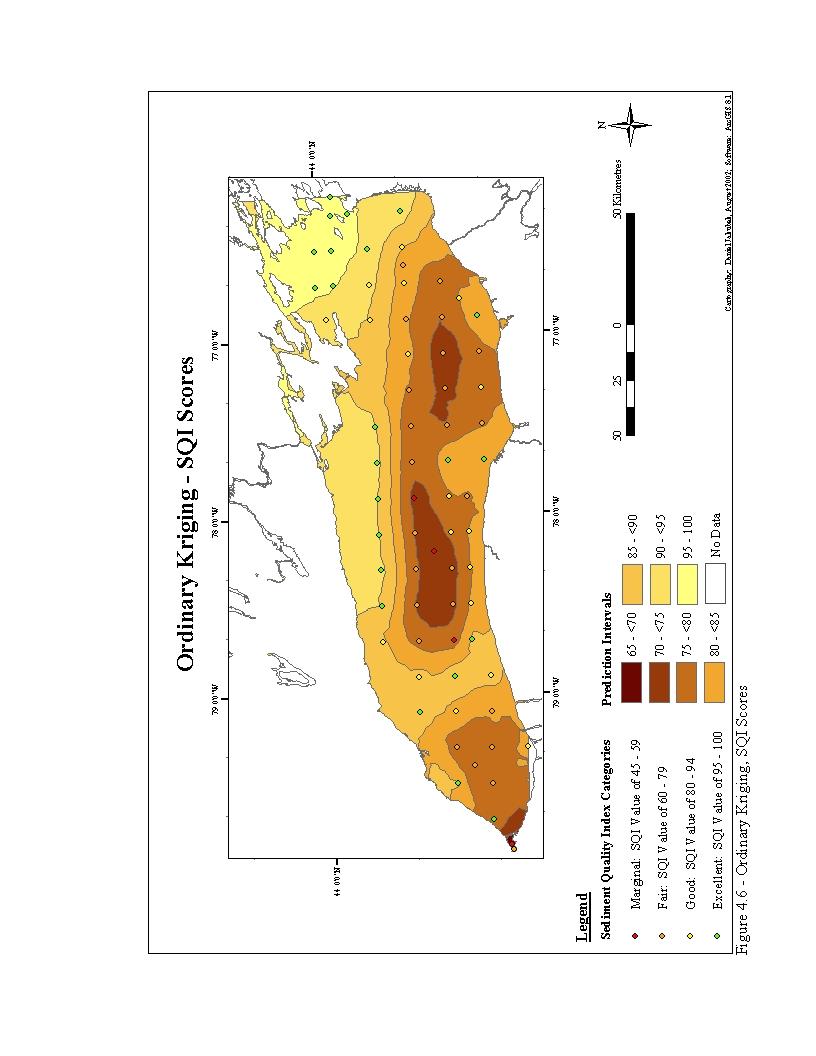
89 77