TECHNICAL MEMORANDUM: MADERA SUBBASIN. Sustainable Groundwater Management Act (SGMA) DRAFT PRELIMINARY BASIN BOUNDARY WATER BUDGET.

Transcription

1 TECHNICAL MEMORANDUM: MADERA SUBBASIN Sustainable Groundwater Management Act (SGMA) DRAFT PRELIMINARY BASIN BOUNDARY WATER BUDGET Prepared by February 2018

2 DRAFT PRELIMINARY Technical Memorandum: Madera Subbasin Sustainable Groundwater Management Act Basin Boundary Water Budget February 2018 Prepared For Madera Subbasin Coordinating Committee Prepared By and Luhdorff and Scalmanini, Consulting Engineers

3 TABLE OF CONTENTS EXECUTIVE SUMMARY INTRODUCTION... 1 WATER BUDGET CONCEPTUAL MODEL... 3 WATER BUDGET ANALYSIS PERIOD... 6 WATER BUDGET DATASETS Surface Water Inflows and Outflows Madera Canal Cottonwood Creek Fresno River Dry Creek Chowchilla Bypass Berenda Creek San Joaquin River Gravelly Ford Canal Inflow and Outflow Data Quality Control Meteorological Data ETo Results Summary Precipitation Results Summary Land Use Crop Water Use Surface Water Diversions Applied Surface Water Groundwater Pumping SURFACE SYSTEM WATER BUDGET ANALYSIS Surface Water System Inflows and Outflows Surface Water System Budget GROUNDWATER SYSTEM WATER BUDGET ANALYSIS DAVIDS ENGINEERING AND LUHDORFF & SCALMANINI i

4 6.1 Approach to Estimating Change in Groundwater Storage and Subsurface Lateral Flows Calculation Analysis Method Regional Model Based Analysis Approach Change in Groundwater Storage Calculated Change in Groundwater Storage Model Based Evaluation of Change in Storage Summary of Change in Groundwater Storage Analysis Subsurface Lateral Flows Calculated Subsurface Lateral Flows Model Based Evaluation of Subsurface Lateral Flows Summary of Subsurface Lateral Flows Analysis PRELIMINARY SUSTAINABLE YIELD ESTIMATES POTENTIAL MANAGEMENT AREAS REFERENCES DAVIDS ENGINEERING AND LUHDORFF & SCALMANINI ii

5 LIST OF TABLES Table ES 1. Preliminary Summary of Sustainable Yield Calculation Results Table 4 1. Preliminary Madera Subbasin Weather Data Time Series Summary for the Period 1989 through 2015 Table 4 2. Preliminary Weather Data Time Series Summary for the Period 1989 through 2015 Table 4 3. Preliminary Water Year Precipitation Statistics for 1989 through 2015 Table 4 4. Preliminary Average Acreages and Annual Evapotranspiration Rates for Madera Subbasin, 1989 To 2015 Table 5 1. Preliminary Annual Averages of Surface Water Inflows from 1989 through 2015 Table 5 2. Preliminary Annual Averages of Surface Water Outflows from 1989 through 2015 Table 5 3. Preliminary Surface Water System Budget (1989 through 2015) in Acre Feet Table 5 4. Preliminary Measured Inflows and Outflows from the Surface Water System Table 5 5. Preliminary Annual Volumes of Surface Water System and Groundwater System Exchanges (1989 through 2015) in Acre Feet Table 6 1. Preliminary Hydrologic Conditions for Selection of Substitute Model Years to Use for 2010 through 2014 Table 6 2. Preliminary Summary of Total Groundwater Elevation Change (ft) Table 6 3. Preliminary Summary of Annual Groundwater Elevation Change (ft) Table 6 4. Preliminary Summary of Calculated Results for Annual Change in Groundwater Storage (AFY) Table 6 5. Preliminary Summary of Model Based Results for Annual Change in Groundwater Storage (AFY) Table 6 6. Preliminary Summary of Calculated and Model Based Results of Change in Groundwater Storage (AFY) Table 6 7. Preliminary Summary of Calculated Results for Annual Subsurface Lateral Flow (C2VSim Kh Estimates) Table 6 8. Preliminary Summary of Calculated Results for Annual Subsurface Lateral Flow (CVHM Kh Estimates) Table 6 9. Preliminary Summary of C2vsim Model Based Results for Annual Subsurface Lateral Flow (AFY) Table 7 1. Preliminary Sustainable Yield Calculated from Groundwater Pumping and Change in Groundwater Storage Table 7 2. Preliminary Sustainable Yield Calculated from Estimated Groundwater Inflows DAVIDS ENGINEERING AND LUHDORFF & SCALMANINI iii

6 Table 7 3. Preliminary Sustainable Yield Calculated from Simulation for Net Recharge from the SWS Equal to Zero Table 7 4. Preliminary Summary of Sustainable Yield Calculation Results Figure ES 1. Preliminary Madera Subbasin GSA Map LIST OF FIGURES Figure ES 2. Preliminary Basin Boundary Water Budget Diagram Figure ES 3. Preliminary Potential Management Areas Based on Hydrogeologic Factors and GSA Boundaries Figure 1 1. Preliminary Madera Subbasin GSA Map Figure 2 1. Preliminary Basin Boundary Water Budget Diagram Figure 2 2. Preliminary Basin Boundary Water Budget (Source: DWR Water Budget BMP (2016)). Figure 3 1. Preliminary Cumulative Departure from Mean Precipitation Figure 4 1. Preliminary Madera Subbasin Inflows and Outflows Figure 5 1. Preliminary Annual Evapotranspiration from 1989 through Figure 6 1. Preliminary Calculated Groundwater Level Changeover Analysis Period ( ) Figure 6 2. Preliminary Specific Yields, Upper Aquifer (C2VSim) Figure 6 3. Preliminary Specific Yields, Upper Aquifer (CVHM) Figure 6 4. Preliminary Horizontal Hydraulic Conductivity (C2VSim) Figure 6 5. Preliminary Horizontal Hydraulic Conductivity (CVHM) Figure 6 6. Preliminary Upper Aquifer Saturated Thickness (C2VSim) Figure 6 7. Preliminary Upper Aquifer Saturated Thickness (CVHM) Figure 6 8. Preliminary Inflow/Outflow Point Pairs & Adjacent Groundwater Subbasins Figure 6 9. Preliminary Modified Madera Subbasin C2vsim CG Model Boundaries for Water Budget Analyses Figure Preliminary Model Based Results for Annual Change in Storage Figure Preliminary Model Based Results for Cumulative Change in Annual Storage Figure Preliminary Calculated Results for Annual Subsurface Lateral Flow Figure Preliminary Calculated Results for Annual Subsurface Lateral Flow from Chowchilla Subbasin Figure Preliminary Calculated Results for Annual Subsurface Lateral Flow from Delta Mendota Subbasin Figure Preliminary Calculated Results for Annual Subsurface Lateral Flow from Kings Subbasin Figure Preliminary Calculated Results for Annual Subsurface Lateral Flow from Merced Subbasin Figure Preliminary Contributing Groundwater Subbasins and Small Watersheds DAVIDS ENGINEERING AND LUHDORFF & SCALMANINI iv

7 Figure Preliminary Model Based Results for Annual Subsurface Lateral Flow Figure Preliminary Model Based Results for Annual Subsurface Lateral Flow Upper Aquifer Figure Preliminary Model Based Results for Annual Subsurface Lateral Flow Lower Aquifer Figure Preliminary Simulated Annual Small Watershed Contribution Figure 8 1. Preliminary Depth to Top of Corcoran Clay Figure 8 2. Preliminary Map of Land Subsidence: 2007 through 2011 Figure 8 3. Preliminary Potential Management Areas Based on Hydrogeologic Factors and GSA Boundaries Figure 8 4. Preliminary Potential Management Areas Based on GSA Boundaries Appendix A Appendix B Appendix C Appendix D Appendix E LIST OF APPENDICES Daily Reference Evapotranspiration and Precipitation Quality Control Madera Subbasin Daily Time Step IDC Root Zone Model Inputs to Support Madera Subbasin Boundary Water Budget ( ) Subbasin Inflow/Outflow Calculations Estimated Values for All Simulated Water Budget Components Based on the Analysis Approach Annual Groundwater Level Change DAVIDS ENGINEERING AND LUHDORFF & SCALMANINI v

8 above normal (AN) acre feet/year (AFY) actual ET (ET a ) air temperature (T a ) alfalfa reference (ET r ) Automatic Weather Stations (AWS) below normal (BN) Best Management Practice (BMP) California Central Valley Groundwater Surface Water Simulation Model (C2VSim) California Data Exchange Center (CDEC) California Department of Water Resources (DWR) California Irrigation Management Information System (CIMIS) Central Valley Hydrologic Model (CVHM) Central Valley Project (CVP) Chowchilla Water District (CWD) Confidence Interval (CI) critical (C) crop ET (ET c ) cubic feet per second (cfs) Davids Engineering (DE) dry (D) LIST OF ABBREVIATIONS ET of applied water (ET aw ) ET of precipitation (ET pr ) evapotranspiration (ET) geographic information system (GIS) grass reference (ET o ) Gravelly Ford (GRF) Gravelly Ford Water District (GFWD) groundwater dependent ecosystems (GDEs) Groundwater Management Plan (GMP) Groundwater Sustainability Agencies (GSA) Groundwater Sustainability Plan (GSP) groundwater system (GWS) hydraulic conductivity (Kh) Hydrogeologic Conceptual Model (HCM) Integrated Water Flow Model (IWFM) Integrated Water Flow Model Demand Calculator (IDC) Luhdorff & Scalmanini Consulting Engineers (LSCE) Madera Irrigation District (MID) Madera Water District (MWD) New Stone Water District (NSWD) Penman Monteith (PM) published coarse grid version of C2VSim, Version R374 (C2VSim CG) reference crop evapotranspiration (ET ref ) relative humidity (RH) Root Creek Water District (RCWD) San Joaquin Valley (SJV) solar radiation (R s ) specific yield (Sy) State Water Resources Control Board (SWRCB) Surface Energy Balance Algorithm for Land (SEBAL) surface water system (SWS) Sustainable Groundwater Management Act of 2014 (SGMA) This Technical Memorandum (TM) U.S. Bureau of Reclamation (USBR) U.S. Department of Agriculture (USDA) United States Geological Survey (USGS) Water Data Library (WDL) wet (W) wind speed (W s ) DAVIDS ENGINEERING AND LUHDORFF & SCALMANINI vi

9 EXECUTIVE SUMMARY Introduction The Madera Subbasin covers about 346,600 acres in Madera County. Seven Groundwater Sustainability Agencies (GSAs) have formed to cover the subbasin in its entirety (Figure ES 1). Groundwater and surface water are critical resources that support agriculture and other economic activities in the subbasin. Groundwater is particularly important because it is relied upon to a significant extent in all years, and serves as the main supply source in periods when surface water supplies are limited. Thus, the sustainable management of groundwater is important to the long term prosperity of Madera County s various communities. The Sustainable Groundwater Management Act of 2014 (SGMA) allows for local control of groundwater resources while requiring sustainable management of these resources. The purpose of this investigation was to develop a preliminary water budget for the subbasin as a whole according to DWR s Groundwater Sustainability Plan (GSP) regulations. This is referred to as the subbasin boundary water budget. The subbasin boundary water budget is based on historical data and is useful because it provides insights into the magnitude of the historical imbalance (or overdraft) of the subbasin. This is turn provides preliminary insights into the nature and scale of potential management actions and/or projects that may be necessary to achieve sustainable groundwater management according to SGMA. Additionally, this work supports initial discussion of delineation of potential management areas. Water Budget Conceptual Model A water budget is defined as a complete accounting of all water flowing into and out of a defined volume (e.g., a subbasin) over a specified period of time. The conceptual model (or structure) for the Madera Subbasin water budget developed for this investigation is consistent with the GSP Regulations and adheres to sound water budget principles and practices (DWR, 2016). The lateral extent of the basin is defined by the subbasin boundaries provided on DWR s groundwater information website (DWR, 2017). The vertical boundaries of the subbasin are the land surface on top and the base of fresh water (Page, 1973) as the bottom of the basin as discussed in the preliminary Hydrogeologic Conceptual Model (HCM) developed during previous data collection and analysis efforts conducted by DE and LSCE (2017). The vertical extent of the basin is subdivided into a surface water system (SWS) and the underlying groundwater system (GWS), with separate but related water budgets prepared for each that together represent the overall subbasin water budget. A conceptual representation of the Madera Subbasin boundary water budget is represented in Figure ES 2. Boundary inflows include precipitation, surface water inflows (in various canals and streams), and boundary watercourse seepage and groundwater inflows from adjoining subbasins. Outflows include evapotranspiration (ET), surface water outflows (in various canals and streams), and groundwater outflows. Also represented in Figure ES 2 are groundwater recharge and extraction, which are internal flows between thesws and GWS. Subbasin boundary inflows and outflows must be quantified according to Section (b) of the GSP Regulations. This was done on a monthly time step for the period 1989 through 2015, including accounting for changes in storage within each time step, such as changes in water stored in the root zone (Equation ES 1). Inflows Outflows = Change in Storage (monthly time step) [ES 1] DAVIDS ENGINEERING AND LUHDORFF & SCALMANINI ES-1

10 FEBRUARY 2018 FIGURE ES-1 Preliminary Madera Subbasin GSA Map DAVIDS ENGINEERING AND LUHDORFF & SCALMANINI ES-2

11 FIGURE ES-2 Preliminary Basin Boundary Water Budget Diagram Separate but related water budgets were prepared for the SWS and GWS. Each budget and associated methodologies and results are documented in the body of this report. Preliminary estimates of subbasin overdraft derived from the SWS and GWS water budgets are briefly described in the following sections. Additionally, discussion of potential management areas is presented. Preliminary Sustainable Yield Estimates for the Subbasin This report estimates an initial Preliminary Sustainable Yield across the entire Madera Subbasin and does not quantify local variability, including the variability between the different GSAs. The preliminary sustainable yield for the overall Madera Subbasin will change once a more detailed analysis is performed. The GSP will quantify local variability among the individual GSAs. Sustainable yield is defined as the maximum quantity of water, calculated over a base period representative of long term conditions (in this case 1989 through 2015) in the subbasin, including accounting for any temporary water surpluses, that can be withdrawn annually from a groundwater supply without causing an undesirable result (CA Water Code 10721). According to DWR s recently released Sustainable Management Criteria BMP (DWR, 2017), Sustainable yield estimates are part of the SGMA s required basinwide water budget and a single value of sustainable yield must be calculated basinwide. For this preliminary analysis, three calculation methods were used to estimate sustainable yield in the Madera Subbasin. The three methods use different combinations of SWS and GWS water budget results to calculate sustainable yield. These preliminary sustainable yield estimates do not include an DAVIDS ENGINEERING AND LUHDORFF & SCALMANINI ES-3

12 evaluation of the spatial distribution of pumping and recharge within the subbasin in relation to sustainability indicators. More detailed analyses will be performed during preparation of the GSP to provide this essential additional detail. The results of all three sustainable yield calculations are similar in magnitude as indicated in Table ES 1. The first method is based on subtracting historical change in groundwater storage from historical pumping, indicating an average sustainable yield of slightly more than 300,000 acre feet annually. The second method is based on summing the total inflow to the GWS, indicating a sustainable yield of slightly less than 300,000 acre feet. Finally, the third method is based on numerical modeling of the subbasin in which water demands are reduced until extraction (pumping) from the subbasin is balanced by recharge. This method also indicates a sustainable yield of slightly more than 300,000 acre feet. The second and third methods each depend on the water budget results and therefore may not be completely independent. These results will be refined during GSP development. Table ES-1 Preliminary Summary of Sustainable Yield Calculation Results Quantification CI Source Method GW pumping and GW Change in Storage Average Volume (AF)* Estimated Confidence Interval (CI) (percent) Average minus CI (AF) Average plus CI (AF) 301,500 16% Calculation 253, ,100 Total Inflows to GWS 298,200 28% Calculation 214, ,400 "Simulation" of 303,100 20% Professional 242, ,700 Reduced Demand Judgement. *1989 through 2014 Based on these preliminary results, which represent recent historical conditions and reflect the 410,000 to 420,000 acre feet of groundwater extractions occurring on average annually in the subbasin, it is estimated that groundwater recharge would need to be increased by approximately 110,000 to 120,000 acre feet annually to achieve sustainable operation of the groundwater system. Alternatively, some combination of increased groundwater recharge and decreased groundwater pumping and water consumption totaling to approximately 110,000 to 120,000 acre feet annually would be needed to achieve sustainable operation of the groundwater system. This preliminary estimate assumes that all other water budget parameters (namely surface water supplies and GWS inflows and outflows) would remain the same in the future as they were during the period of analysis. More detailed analysis during GSP preparation will assess the reasonableness and validity of these assumptions, taking into account climate change and other possible changes. Potential Management Areas Potential management areas were considered in terms of hydrogeologic features and jurisdictional boundaries, and some options are presented. Based on review of the preliminary HCM, the key hydrogeologic features of Madera Subbasin include the extent of Corcoran Clay and the extent and magnitude of historical subsidence. The key jurisdictional boundaries to consider are the GSA boundaries. Regardless of the ultimate decision made by the GSAs regarding boundaries for management areas, individual SWS water budgets are planned for each GSA to provide greater insight on water inflows and outflows at the GSA boundary scale. DAVIDS ENGINEERING AND LUHDORFF & SCALMANINI ES-4

13 One potential option to consider for management areas that involves consideration of both hydrogeologic factors and GSA boundaries would involve delineation of three management areas in the western, central, and eastern portions of the subbasin (Figure ES 3). The western management area would encompass the area where Corcoran Clay is present and the area of the subbasin most impacted by historical subsidence. GSAs in the western area include all Gravelly Ford Water District (GFWD), all of New Stone Water District (NSWD), portions of Madera County, and portions of Madera Irrigation District (MID). The central management area would be immediately east of the Corcoran Clay and has shown minimal historical subsidence. The City of Madera GSA is entirely contained in the central area, but the majority of the central area is occupied by the MID GSA. The potential eastern area is far removed from the Corcoran Clay and any significant subsidence concerns. It includes all of Madera Water District GSA and Root Creek Water District GSA, but the majority of the eastern area lands are part of Madera County GSA. A second potential option is to have management areas based solely on GSA boundaries with no consideration of hydrogeologic factors. This option would result in non contiguous management areas given the nature of GSA boundaries. However, using GSA boundaries to delineate management areas would allow each GSA to have a better understanding of its own particular Basin Setting (e.g., geologic conditions, water budget, groundwater conditions). The recommended next step in the management area development process is further discussion among the GSAs regarding advantages and disadvantages of the two options described. Limitations of This Preliminary Analysis The main limitation of this preliminary basinwide analysis is that it does not account for all undesirable results and does not consider potential localized undesirable effects. An additional limitation is the reliance at this preliminary stage of investigation on the coarse grid Central Valley groundwater model, and its somewhat dated period of analysis, to estimate changes in groundwater storage, and groundwater inflows and outflows. During GSP development a finer grid local model will be developed that will consider all undesirable and localized undesirable results as required by the GSP regulations. DAVIDS ENGINEERING AND LUHDORFF & SCALMANINI ES-5

14 FEBRUARY 2018 FIGURE ES-3 Preliminary Potential Management Areas Based on Hydrogeologic Factors and GSA Boundaries DAVIDS ENGINEERING AND LUHDORFF & SCALMANINI ES-6

15 INTRODUCTION Agriculture is an important economic driver in the Madera area and groundwater represents an important source of supply for agricultural, municipal, domestic and industrial uses in the Madera Subbasin. Thus, the sustainable management of groundwater is important for the long term prosperity of the community. The Sustainable Groundwater Management Act (SGMA) allows for local control of groundwater resources while requiring sustainable management of these resources. The Madera Subbasin covers approximately 346,600 acres, all within Madera County. Seven Groundwater Sustainability Agencies (GSA) have formed to cover the subbasin (Figure 1 1). The largest of these is the Madera County GSA covering about 176,800 acres. The Madera Irrigation District (MID) GSA covers about 134,100 acres in Madera County. The remainder of the subbasin is covered by five additional GSAs, including the City of Madera GSA, Root Creek Water District (RCWD) GSA, Gravelly Ford Water District (GFWD) GSA, New Stone Water District (NSWD) GSA, and Madera Water District (MWD) GSA, each individually covering areas between about 3,700 and 10,000 acres. The Madera Subbasin has been identified by the California Department of Water Resources (DWR) as a critically overdrafted subbasin. Davids Engineering (DE) and Luhdorff & Scalmanini Consulting Engineers (LSCE) recently completed the Sustainable Groundwater Management Act (SGMA) Data Collection and Analysis project for the Madera Subbasin Coordinating Committee. This technical memorandum (TM) documents another task identified by the Madera Subbasin Coordinating Committee as an initial step towards addressing SGMA requirements and the development of a Groundwater Sustainability Plan (GSP). The Committee requested that the DE and LSCE Team complete selected tasks identified during the Data Collection and Analysis Project, including completion of a basin boundary water budget and development of a preliminary basin wide estimate of sustainable yield. Importantly, the water budget and sustainable yield estimates are preliminary and do not include assessment of undesirable results as required by the GSP regulations. Furthermore, the boundary water budget represents the subbasin in aggregate and therefore the preliminary estimate of sustainable yield does not account for possible localized undesirable results within the subbasin. The objectives of this study are to conduct an initial evaluation of the available data relating to water budget components within the Madera Subbasin and to prepare preliminary assessments of sustainable yield and potential management areas to support future analyses to be conducted as part of development of a GSP for the Madera Subbasin. DWR has recently published guidance and Best Management Practice (BMP) documents related to the development of GSPs (DWR, 2016). The GSP Annotated Outline includes four distinct components for the Basin Setting section: Hydrogeologic Conceptual Model (HCM), Current and Historical Groundwater Conditions, Water Budget Information, and Management Areas. This TM documents a systematic process to prepare and analyze data relating to the historical water budget, sustainable yield and evaluation of potential options for management areas for the Madera Subbasin. This TM includes sections describing the conceptual water budget, water budget analysis period, water budget data sources and data acquired, boundary water budget assembly, groundwater storage change calculations, groundwater inflow and outflow calculations, the boundary water budget assembly, a preliminary sustainable yield analysis, and a preliminary delineation of management areas. The methods of analysis, results and, importantly, limitations of the aggregated water budget, preliminary sustainable yield and potential management areas for the Madera Subbasin area are presented to help inform more detailed water budget analyses and the more detailed sustainable yield analysis (including consideration of undesirable results) to be conducted as part of the GSP development. DAVIDS ENGINEERING AND LUHDORFF & SCALMANINI 1

16 FEBRUARY 2018 FIGURE 1-1 Preliminary Madera Subbasin GSA Map DAVIDS ENGINEERING AND LUHDORFF & SCALMANINI 2

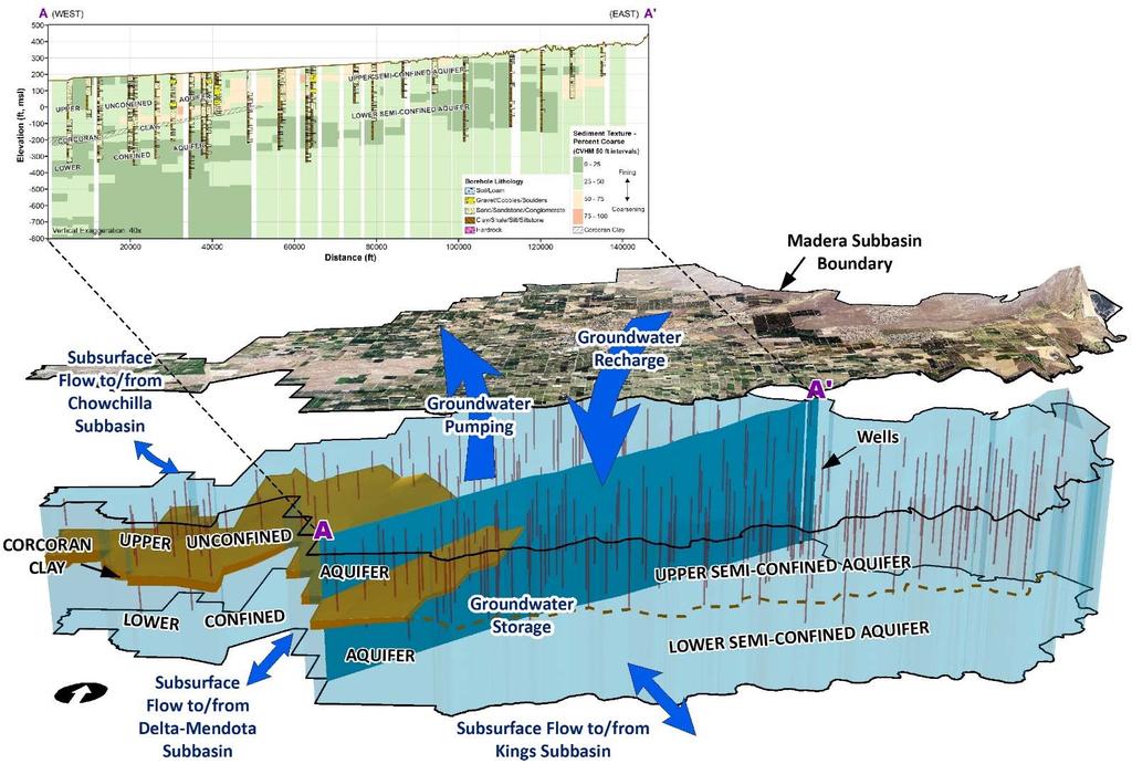
17 WATER BUDGET CONCEPTUAL MODEL A water budget is defined as a complete accounting of all water flowing into and out of a defined volume (e.g., a subbasin) over a specified period of time. The conceptual model (or structure) for the Madera Subbasin water budget was developed during previous data collection and analysis efforts conducted by DE and LSCE (2017) and is consistent with the GSP Regulations and adheres to sound water budget principles and practices described in the Water Budget BMP (DWR, 2016). The lateral extent of the basin is defined by the subbasin boundaries provided in the recent DWR Bulletin 118 update (DWR, 2016). The vertical boundaries of the subbasin are the land surface on top and the definable bottom of the basin. The definable bottom was established as part of developing the preliminary HCM during previous data collection and analysis efforts conducted by DE and LSCE (2017). The vertical extent of the basin is subdivided into a surface water system (SWS) and groundwater system (GWS), with separate but related water budgets prepared for each that together represent the overall subbasin water budget. The SWS represents the land surface down to the bottom of plant root zone, within the lateral boundaries of the basin. The GWS extends from the bottom of the root zone to the definable bottom of the subbasin, within the lateral boundaries of the basin. The SWS basin boundary water budget was completed on a monthly time step and calendar year 1 annual results are provided in Section 5. The SWS is further subdivided into water use sectors identified in the GSP regulations. Water use sectors are defined in the GSP Regulations as categories of water demand based on the general land uses to which the water is applied, including urban, industrial, agricultural, managed wetlands, managed recharge, and native vegetation. Water budgets for each water use sector in the subbasin will be added to the water budget during GSP development. Subbasin boundary inflows and outflows must be quantified according to Section (b) of the GSP Regulations. Inflows and outflows may cross the subbasin boundary, or may represent exchanges of water between the SWS and the underlying GWS. The Madera Subbasin boundary water budget is represented in Figure 2 1. Boundary inflows include precipitation, surface water inflows (in various canals and streams), boundary watercourse seepage and groundwater inflows from adjoining subbasins. Outflows include evapotranspiration (ET), surface water outflows (in various canals and streams), and groundwater outflows. Also represented in Figure 2 1 are groundwater recharge and extraction, which are internal flows between the SWS and GWS. Net recharge from the SWS from the GWS is defined as groundwater recharge minus groundwater extraction, and is useful for understanding and analyzing the combined effects of land surface processes on the underlying GWS. Basin boundary inflows and outflows are quantified on a monthly basis, including accounting for any changes in storage, such as changes is water stored in the root zone (Equation 2 1). Inflows Outflows = Change in Storage (monthly time step) [2 1] 1 Calendar years represent the agricultural irrigation season better than water years. DAVIDS ENGINEERING AND LUHDORFF & SCALMANINI 3

18 Precip ET Madera Subbasin SW Outflows Surface Water System (SWS) (change in storage) SW Inflows San Joaquin River Riparian Diversions and Seepage GW Outflows Groundwater System (GWS) (change in storage) Net Recharge from the SWS = GW Recharge - GW Extraction GW Inflows FIGURE 2-1 Preliminary Basin Boundary Water Budget Diagram A slightly more detailed representation of the conceptual budget from DWR s water budget BMP document (DWR 2017) is shown in Figure 2 2. It is conceptually identical to Figure 2 1, but illustrates the various inflows and outflows comprising recharge, extraction and discharge from the GWS. FIGURE 2-2 Preliminary Basin Boundary Water Budget (Source: DWR Water Budget BMP (2016)) DAVIDS ENGINEERING AND LUHDORFF & SCALMANINI 4

19 The time period of analysis selected for the water budget analysis is discussed in Section 3. The specific components of SWS inflows and outflows, and the data available and calculation methodology for each component are described in Section 4, with water budget results presented in Section 5. Quantification of GWS inflows and outflows is described in Section 6. Inflows and outflows were calculated independently using measurements and other data, or calculated as the water budget closure term. DAVIDS ENGINEERING AND LUHDORFF & SCALMANINI 5

20 WATER BUDGET ANALYSIS PERIOD In accordance with GSP regulations, a base period must be selected so that the analysis of sustainable yield is performed for a representative period, with minimal bias that might result from the selection of an overly wet or dry period, while recognizing changes in other conditions including land use and water demands. The base period should be selected considering the following criteria: long term mean annual water supply; inclusion of both wet and dry periods, antecedent dry conditions, adequate data availability; and inclusion of current hydrologic, cultural, and water management conditions in the basin. To develop a preliminary base period to be used for sustainability analyses during GSP development, only historical precipitation records for the area were evaluated. Precipitation provides an indication of the long term mean water supply and potential for natural groundwater recharge. Monthly precipitation records acquired from the Western Regional Climate Center for a station in Madera (Station ) were analyzed for the period 1928 through This station provides a longer record than the CIMIS weather stations described in Section 4. A plot with annual precipitation, mean annual precipitation, and cumulative departure 2 from mean annual precipitation was developed for the Madera station (Figure 3 1). Notable on this plot is the long term overall average period from the late 1920s through the late 1970s (overall flat cumulative departure curve), followed by a somewhat wet period during the late 1970s and early 1980s, dry late 1980s, wet 1990s, overall average from late 1990s through 2011, and recently a dry period from 2012 through The period of 1989 through 2015 is a relatively balanced climatic period with a similar number of wet and dry years and some prolonged periods of wet, dry, and average conditions and represents a reasonable base period for conducting sustainability analyses. Nevertheless, the net negative slope of the cumulative departure curve over this period suggests that precipitation inputs to the subbasin over the 1989 through 2015 period were slightly below average (relative to the entire 1928 through 2015 period average). Antecedent (i.e., prior or left over year) dry conditions minimize differences in groundwater in the unsaturated zone at the beginning and at the end of a study period. Given that the measure of water in the unsaturated zone is nearly impossible to determine, particularly at the scale of a groundwater subbasin, selection of a base period with relatively dry conditions antecedent to the beginning and end of the period of record is preferable because any water stored in the unsaturated zone is minimized. In this case, the proposed base period from 1989 through 2015 begins in a dry year with one additional prior dry year and ends in a dry year with several prior dry years. The available hydrologic and land and water use data over the period are sufficient to calculate the various parameters used to analyze groundwater conditions as related to the groundwater budget and sustainability (e.g., precipitation, streamflow, land uses, groundwater pumping, groundwater levels, and imported water sources). Lastly, the proposed base period ends near the present time, and therefore can be used to assess groundwater conditions as they currently exist. Given these criteria, the base period of 1989 through 2015, is considered to be appropriate for assessing groundwater conditions with minimal bias introduced from land use changes or imbalances due to wet or dry conditions. Although the evaluation of the precipitation data at Madera suggest that 1989 through 2015 represents a good base period of 27 years for conducting GSP analyses, additional consideration with respect to the base 2 Cumulative departure curves are useful to illustrate long term rainfall characteristics and trends during drier or wetter periods relative to the mean annual precipitation. Downward slopes of the cumulative departure curve represent drier periods relative to the mean, while upward slopes represent a wetter period relative to the mean. DAVIDS ENGINEERING AND LUHDORFF & SCALMANINI 6

21 period should be given during the GSP development as additional data review is conducted. In particular, consideration should be given to the patterns of CVP supplies and to local supplies from Hensley Lake, which may or may not be strongly correlated with local precipitation. Ultimately, the GSP base period may be selected based on some combination of these and/or other factors to define a period that is normal for the subbasin from a water budget perspective. The GSP regulations also specify that sustainability analyses be conducted on at least an annual time step. However, a monthly time step is recommended to support evaluation of sustainability indicators, and potential projects and management actions. These sustainability evaluations, which may include analyses involving hydrologic modeling, will require data and analyses at a time step sufficient to assess seasonal conditions and trends within an annual interval in addition to long term trends spanning years. The analysis period selected for this initial water budget evaluation is based on a combination of the historical climatic conditions and availability of data suitable for use in conducting the different analyses of the water budget components. During review of groundwater level data needed to calculate change in groundwater storage from observed conditions, it became apparent that 1989 through 2014 would be a more appropriate analysis period for this effort because of the relative sparsity of groundwater level data (and therefore diminished quality of resulting groundwater level interpretations) available for Therefore, the analysis results discussed below are based on analysis of the period 1989 through 2014, although data and calculations of water budget components were also assembled for 2015, to the extent that suitable data exist. Based on the cumulative departure curve (Figure 3 1) used to choose time periods for analysis, using 2014 as the last year still provides a balanced hydrologic time period for the analysis. Therefore, groundwater elevation contours were produced for spring of 2014, and used for change in groundwater levels and change in storage calculations. The GSP regulations require that evaluation of water budgets under projected future conditions utilize 50 years of historical hydrology (precipitation, evapotranspiration and streamflow) information. Evaluation of projected future water budgets for the Madera Subbasin was not part of this analysis and will be conducted as part of future GSP development efforts. DAVIDS ENGINEERING AND LUHDORFF & SCALMANINI 7

22 FIGURE 3-1 Preliminary Cumulative Departure from Mean Precipitation DAVIDS ENGINEERING AND LUHDORFF & SCALMANINI 8

23 WATER BUDGET DATASETS This section describes the data sources, quality control and calculations completed to develop the main time series datasets required to develop the SWS water budget. The datasets include surface water inflows and outflows, meteorological data used to compute reference crop evapotranspiration (ET ref ), land use and cropping patterns, crop water use (evapotranspiration, or ET), surface water diversions, applied surface water volumes, and groundwater pumping volumes. Each of these datasets is described below. 4.1 Surface Water Inflows and Outflows Madera Canal Inflow data for the Madera Canal were assembled from measurements collected by the United States Geological Survey (USGS) for the MADERA CN A FRIANT CA site. This site is located near the town of Friant, California is also referred to by its USGS site number: This site measures the flow in the Madera Canal just downstream of the diversion point from Millerton Lake near the north end of Friant Dam. This water is used to irrigate lands in the Madera and Chowchilla Subbasins. Daily records of discharge in cubic feet per second (cfs) were downloaded for the full period of available records, from October 1, 1948 through September 30, These 68 years of records were summarized into monthly and annual volumes. The Madera Canal enters the Madera Subbasin at its southeastern corner, runs northwesterly along the eastern subbasin boundary, and leaves the subbasin almost 32 miles to the northwest. Located along the canal are delivery points to irrigation distribution infrastructure and irrigated lands within the Madera Subbasin. The USGS inflow measurement site described above is located 0.58 miles outside of the subbasin boundary. More information about this site is available at: Outflow data for the Madera Canal were assembled from records provided by MID for the years using the data from operating reports of Class 1 and Class 2 Deliveries to MID and Chowchilla Water District (CWD). These data were assembled into monthly and annual volumes. Irrigation deliveries from the Madera Canal to the MID distribution system and in some cases directly to MID irrigated lands were compiled into monthly and annual volumes using data provided by MID. These deliveries were included as surface water inflow into the Madera Subbasin. Using the USGS Madera Canal inflow data and the irrigation deliveries to MID and to CWD, a monthly water budget for the Madera Canal was prepared to estimate seepage from the canal. For this preliminary seepage estimate, canal evaporation was assumed to be negligible. Seepage estimates for the Madera Canal prepared for the Madera Canal Capacity Restoration Feasibility Study (USBR 2016) were also reviewed. For this preliminary water budget, the seepage estimate of 5,400 acre feet for the full canal length was multiplied by 87 percent, the percent of the canal length in, or on the boundary, of the Madera Subbasin. DAVIDS ENGINEERING AND LUHDORFF & SCALMANINI 9

24 FIGURE 4-1 Preliminary Madera Subbasin Inflows and Outflows DAVIDS ENGINEERING AND LUHDORFF & SCALMANINI 10

25 4.1.2 Cottonwood Creek Inflow data for Cottonwood Creek were assembled from records provided by MID. MID has installed a number of recorders within the district infrastructure that record flows at key inflow and outflow points. One of these points is Recorder 14: Cottonwood Creek Head, which records historical inflows. The recorder is located along the creek just a few miles southeast of Madera, CA in Madera County. Average daily flow volumes were provided by MID for the years , and summarized into monthly and annual volumes. Cottonwood Creek enters the Madera Subbasin along its eastern boundary, and continues for approximately 34 miles through the subbasin until it exits along the southwestern subbasin boundary. During the irrigation season, just over 18 miles of the creek are used as part of the irrigation distribution system. The measurement point of Recorder 14 is approximately 11 miles from the eastern boundary of the subbasin. The measured flows at this point have been used as an estimate of the flows entering the Madera Subbasin; for this preliminary water budget, no adjustment for seepage loss from the portion of the canal outside the subbasin has been completed. Additionally, Gravelly Ford Water District diverts water from Cottonwood Creek downstream of MID Recorder 10 under water right Application A Permit # Fresno River Inflow data for the Fresno River were assembled from records provided by both the USGS and the DWR s California Data Exchange Center (CDEC). The USGS site named FRESNO R BL HIDDEN DAM NR DAULTON CA, is located near Daulton, CA in Madera County, approximately 1 mile downstream of Hidden Dam on the Fresno River. The site is also referred to by its USGS site number: This site measures discharge in the Fresno River at this point and has discharge records for the period October1941 through October The CDEC site, Hidden Dam (Hensley), is also located near Daulton, CA in Madera County just downstream of Hidden Dam. This site also measures the discharge of the reservoir in the Fresno River and has records for October 1993 through present. Data sets from both sites were downloaded and summarized into monthly and annual volumes. The Fresno River enters the Madera Subbasin along its eastern boundary and exits along its western boundary. The total distance of the river within the subbasin boundaries is approximately 27 miles. During the irrigation season, about 10 miles of the river are used as part of the irrigation water distribution system. The inflow measurement points are approximately 2 miles upstream of the subbasin boundary. The measured flows at this point were used as an estimate of the flows entering the Madera Subbasin. Additional information about this site can be found by visiting progs/stationinfo?station_id=hid or Outflow data for the Fresno River was assembled from records provided by MID for Recorder 4: Fresno River Rd. 16. This recorder measures flow in the Fresno River where it exits the MID service area, approximately 10 miles directly west of the City Madera. Average monthly and daily flow volumes were provided by MID for the years From these records, monthly and annual summaries of volumes were compiled. This measurement point is approximately 4 miles inside of the subbasin boundary. In this preliminary water budget, the measured flows at this point were used as an estimate of the flows leaving the Madera Subbasin, without adjustment for seepage loss from the portion of the river inside the subbasin but downstream of the outflow measurement point. On rare occasions, Fresno River flows may be diverted up Dry Creek to satisfy irrigation demands. Historical information DAVIDS ENGINEERING AND LUHDORFF & SCALMANINI 11

26 documenting when these infrequent diversions occurred is unavailable. These flows will be further investigated during GSP development Dry Creek Inflow data for Dry Creek were assembled from records provided by MID. Another recorder within their system, Recorder 5: Dry Creek Head Flood Water, is located along Dry Creek approximately 7 miles north of the City of Madera. Average daily flow values were provided by MID for the years 1966 through 2017, which were summarized into monthly and annual flow volumes. Dry Creek enters the Madera Subbasin along the eastern border, between the Fresno River and Berenda Creek. It travels for a distance of approximately 24 miles before its confluence with the Fresno River before the Fresno River reaches the subbasin boundary. About 21 of the 24 miles of this waterway are used as part of the irrigation distribution system during the irrigation system. The measured flows at Recorder 5, approximately 8.5 miles inside the boundary of the subbasin, were used as an estimate of the flows entering the Madera Subbasin; For this preliminary water budget no adjustment for seepage loss from the portion of the creek inside the subbasin but upstream of the inflow measurement point was completed. Dry Creek joins the Fresno River before the measurement at MID Recorder 4. Therefore, Dry Creek outflow is usually included in the Fresno River outflow measurement. However, sometimes during flood conditions, the Sallaberry Canal often conveys Dry Creek flows out of the Subbasin without passing through Recorder 4 in the Fresno River. This outflow will be included with an estimate of the flows during GSP development Chowchilla Bypass The Chowchilla Canal Bypass is located along the southern edge of the Madera Subbasin. It is a flood control channel operated via gates along the San Joaquin River that are opened to divert flow into the bypass when flow in the San Joaquin River would exceed the river s downstream capacity. The bypass may remain dry for extended periods of time until needed to convey flood flows and provide flood protection. At other times of the year, water may remain ponded in some of the lower lying areas. Because of these characteristics and the fact that this site is operated on an as needed basis, there may be significant times during the record of flow that there is no water flowing through the channel. Records like this are denoted as Below the Rating Table in the DWR s CDEC and were replaced with 0 before proceeding with the compilation of monthly and annual volumes. Inflow data for Chowchilla Bypass at head Below Control Structure were assembled using a combination of CDEC records and DWR s Water Data Library (WDL) records. WDL provided data for the years , and CDEC provided data for the years Daily average flow values were summarized as monthly and annual volumes for this site. The Chowchilla Bypass enters the Madera Subbasin along the southwestern border, traverses the Subbasin for approximately 5 miles, and exits the subbasin boundary and enters the Chowchilla Subbasin. It flows intermittently, only when flows in the San Joaquin River are above flood stage. Shortly after exiting the subbasin boundary, the Fresno River flows into the Bypass. At this point it becomes the Eastside Bypass. There is no measurement point for flows leaving the Madera subbasin in the Chowchilla Bypass. Seepage and evaporation losses from the Chowchilla Bypass for the five mile length in the Madera Subbasin have been assumed to be negligible for this preliminary water budget. To track the Chowchilla Bypass flows, the measured flows at the Chowchilla Bypass at head Below DAVIDS ENGINEERING AND LUHDORFF & SCALMANINI 12

27 Control Structure have been used as an estimate of the flows entering the Madera Subbasin and leaving the Madera Subbasin, without adjustment for seepage loss Berenda Creek Inflow data for Berenda Creek were assembled from records provided by MID. Another recorder within their system, Recorder 13: Berenda Creek Head, is located along Berenda Creek approximately 7.5 miles north of the City of Madera. Average daily flow values were provided by MID for the years 1970 through 2017, and summarized into monthly and annual flow volumes. Berenda Creek enters the Madera Subbasin along the northeastern subbasin boundary, between the Chowchilla River and Dry Creek. It continues southwesterly for a distance of approximately 28 miles before exiting the subbasin boundary just north of the Fresno River. During the irrigation season, approximately 7.5 miles of this waterway are used as part of the irrigation distribution system. The inflow measurement point is almost 13 miles inside the boundary of the subbasin, as measured along the course of the creek. In this preliminary water budget, the measured flows at this point have been used as an estimate of the flows entering the Madera Subbasin, without adjustment for seepage loss from the portion of the creek within the subbasin but upstream of the inflow measurement point. Outflow data for Berenda Creek were assembled from records provided by MID for Recorder 2: Berenda Creek Spill, located along Berenda Creek approximately 8.5 miles south of the City of Chowchilla. Monthly and daily flow volumes were provided by MID for the years 1966 through 2017, and were compiled into monthly and annual volume summaries. Berenda Creek exits the Madera Subbasin along its western edge, just north of the Fresno River. The measurement point for this recorder is just over 3 miles upstream of the subbasin boundary. In this preliminary water budget, the measured flows at this point have been used as an estimate of the flows leaving the Madera Subbasin, without adjustment for seepage loss from the portion of the creek inside the subbasin but upstream of the inflow measurement point San Joaquin River Inflow data for the San Joaquin River were assembled from records provided by the USGS. The site, called SAN JOAQUIN R BL FRIANT CA, is located near the town of Friant in Fresno County, approximately 2 miles downstream of the Friant Dam. This site is also referred to by its site number: The site measures flows released from Millerton Lake. Discharge records are available for nearly 110 years, from 1911 to the present. Daily data was downloaded and summarized into monthly and annual volumes. The San Joaquin River runs southwesterly from Millerton Lake north of the northern edge of the City of Fresno, then travels westward toward the City of Mendota, forming the southern Madera Subbasin boundary. It exits the subbasin approximately 8 miles northwest of the City of Kerman. The total length of the river along the subbasin boundary is nearly 40 miles. The San Joaquin River below Friant measurement point is 0.5 miles inside the subbasin boundary. Additional information about this site is available at: Outflow data for the San Joaquin River were assembled from records provided by CDEC. The site, named San Joaquin River at Gravelly Ford (GRF), is located in Madera County approximately 7.5 miles northwest of the town of Kerman. The site measures mean daily flow values with data available for the DAVIDS ENGINEERING AND LUHDORFF & SCALMANINI 13

28 period from 6/27/1997 to the present. The data were downloaded and summarized as monthly and annual volumes. The San Joaquin River leaves the Madera Subbasin boundary 0.7 miles downstream of this measurement point, and the Gravelly Ford Canal Pumped Diversion inflow is just over one mile upstream of the measurement site. More information about this site is available at: progs/stameta?station_id=grf. Based on a list of riparian diversions and estimates of capacity between Friant and Gravelly Ford (McBain & Trush, 2002), an estimate of the area irrigated was prepared. The almond applied water results from the root zone water budget described later in Section 5 was used with the area to estimate riparian diversions. During the GSP preparation, this estimate will be checked by totaling the cropped area riparian to the river from the land use analysis described in Section 5. Riparian deliveries are inflows to the basin and were included in the surface water inflows. Using the USGS San Joaquin River below Friant flow data, the inflow from Little Dry Creek, the Gravelly Ford discharge measurement site and the estimate of riparian diversions, a water budget for this reach of the San Joaquin River was completed to estimate the volume of river seepage. For this preliminary estimate of seepage, evaporation was assumed to be negligible. San Joaquin River seepage is an inflow to the GWS and is included in the infiltration of surface water. McBain & Trush (2002) also estimated San Joaquin River seepage. These estimates will be reviewed during the GSP development studies Gravelly Ford Canal The Gravelly Ford Canal is pumped from the San Joaquin River at a site known as the Gravelly Ford Pump Diversion. The Gravelly Ford Water District (GFWD) provided pumping volumes for the years This pumping site is located along the San Joaquin River just over 1 mile upstream of the San Joaquin River at Gravelly Ford USGS measurement site. The records provided by GFWD were assembled into monthly and annual volumes Inflow and Outflow Data Quality Control Quality control procedures were applied to identify data gaps and data values outside of plausible ranges. Data gaps were filled with estimates based on the water year index ( progs/iodir/wsihist) developed by the DWR. DWR has categorized each water year since 1901 for both the Sacramento and San Joaquin Valleys into five year types based on estimated unimpaired runoff. DWR defines unimpaired runoff as the natural water production of a river basin, unaltered by upstream diversions, storage, and export of water to or import of water from other basins. Each year is assigned one of the following five year types: wet (W), above normal (AN), below normal (BN), dry (D), and critical (C). For months with missing data within the years , the average of that same month calculated using all the years with the same water year classification was used as an estimate for the flow in the missing month. When the number of years with available data for developing water year type monthly averages was less than five, the five water year types were grouped into simply Wet and Dry years. Wet years were defined as wet or above normal, and the Dry years were defined as below normal, dry, or critical. DAVIDS ENGINEERING AND LUHDORFF & SCALMANINI 14

29 4.2 Meteorological Data ETo Results Summary A scientifically sound and widely accepted method for determining consumptive use of irrigation water utilizes daily reference crop evapotranspiration (ET ref ) values calculated using the standardized Penman Monteith (PM) method as described by the ASCE Task Committee Report on the Standardized Reference Evapotranspiration Equation (ASCE EWRI, 2005). The PM method requires measurements of the following meteorological (weather) parameters: incoming solar radiation (R s ), air temperature (T a ), relative humidity (RH) and wind speed (W s ), all at hourly or daily time steps. The task committee report standardizes the ASCE PM method for application to a full cover alfalfa reference (ET r ) and to a clipped cool season grass reference (ET o ). The clipped cool season grass reference is widely used throughout the western United States and was selected for this application. Additionally, the Task Committee Report provides recommended methods for estimating required inputs to the standardized equation when measured data are missing. Weather data from irrigated areas are needed to develop estimates of consumptive use of irrigation water. Automatic Weather Stations (AWS) provide measurements of R s, T a, RH and W s over hourly or shorter periods used to compute ET o. The California Irrigation Management Information System (CIMIS) weather stations meet these requirements and weather data was obtained and quality controlled to develop ET ref and precipitation records for the Madera Subbasin for the period from 1989 through Table 4 1 lists the stations and periods of record used. Table 4-1 Preliminary Madera Subbasin Weather Data Time Series Summary for the Period 1989 through 2015 Weather Station Start Date End Date Comment Fresno State Oct. 2, 1988 May 12, 1998 CIMIS. Before Madera was installed. Madera May 13, 1998 Apr. 2, 2013 Madera II Apr. 3, 2013 Dec. 31, 2015 CIMIS CIMIS. Moved eastward 2 miles in 2013 and renamed Madera II. Weather data from each station were reviewed and corrected when necessary following accepted, scientific procedures (Allen et al., 1996; Allen et al., 1998; ASCE EWRI, 2005; and ASCE, 2016). Daily data were checked using visual interpretation of time series graphs developed in spreadsheets. Quality control methods according to the guidelines specified in Appendix D of the ASCE Task Committee Report on the Standardized Reference Evapotranspiration Equation (ASCE EWRI, 2005) were applied as necessary, as described in Appendix A. The average water year ET o for 1989 through 2015 was inches and ranged from inches in 1995 to inches in 2004 (Table 4 2). DAVIDS ENGINEERING AND LUHDORFF & SCALMANINI 15

30 Table 4-2 Preliminary Weather Data Time Series Summary for the Period 1989 through 2015 Average Minimum Maximum Water Weather Start Date End Date Water Year Water Year Year ET o, inches Station ET o, inches ET o, inches Fresno State Oct. 2, 1988 May 12, (1995) (1992) Madera May 13, 1998 Apr. 2, (2011) (2004) Madera II Apr. 3, 2013 Dec. 31, (2014) (2015) Overall Oct. 2, 1988 Dec. 31, (1995) (2004) Water year ET o totals for the complete 1989 through 2015 period are included in Appendix A Precipitation Results Summary Based on data from the same weather stations described above, the 27 year average water year precipitation from 1989 through 2015 was inches, varying from 3.59 inches in 2014 to inches in 1995 (Table 4 3). Table 4-3 Preliminary Water Year Precipitation Statistics for 1989 through 2015 Average Minimum Maximum Water Weather Water Year Water Year Year Start Date End Date Station Precipitation, Precipitation, Precipitation, inches inches inches Fresno State Oct. 2, 1988 May 12, (1994) (1995) Madera May 13, 1998 Apr. 2, ( (2006) Madera II Apr. 3, 2013 Dec. 31, (2014) 4.90 (2015) Overall Oct. 2, 1988 Dec. 31, (2014) (1995) Water year precipitation totals for the complete 1989 through 2015 period are included in Appendix A. 4.3 Land Use Accurate land use areas are required for determining consumptive use of irrigation water, or evapotranspiration (ET). The objective was to develop a Madera County wide annual, spatial crop acreage dataset from which the crop areas in the Madera Subbasin, Madera County GSA in Madera Subbasin, MID GSA, RCWD GSA, Gravelly GFWD GSA, NSWD GSA and Madera City GSA were derived. Data used to develop annual, county wide spatial land use includes: (1) DWR spatial land use surveys for Madera County in 1995, 2001 and 2011, (2) Land IQ 3 remotely sensed land use data obtained through 3 Land IQ is a firm that was contracted by DWR to use remote sensing methodologies to identify crops in fields. DAVIDS ENGINEERING AND LUHDORFF & SCALMANINI 16

31 DWR for 2014, and (3) Madera County Agricultural Commissioner annual crop production areas reported for 1989 through The following five steps were taken: 1.) Developed spatial land use coverages for 1995, 2001, 2011, and Made adjustments to the spatial coverage, including: a) Inserted 2011 DWR coverage for missing areas from 2014 LandIQ coverage (native, urban, water, & semi agriculture land uses account for 86% of the missing area) b) Water surfaces were not included in the 1995 DWR survey; used the water area from 2001 for the 1995 DWR survey 2.) Calculated agricultural area: a) County data have idle equal to zero for all years assumed county data do not include idle land b) Excluded idle from DWR agricultural totals to be consistent with county totals c) Calculated the ratio of the DWR agricultural total area (not including idle lands) to county agricultural production area for years with DWR (or Land IQ) land use data d) Interpolated the ratio calculated in step (c) for missing years, extended trend or set at last values for years before first and after last county data 3.) Multiplied county agricultural acres for each crop by the ratio calculated in step 2 (c) to adjust county agricultural areas for each crop scaling each crop area in each year by an estimate of the difference between the areas in the DWR land use surveys and County Commissioner reports. This procedure assumes DWR areas are the most accurate. a) Interpolated native, semi agriculture, urban, and water land uses between DWR years b) Calculated idle area as the remaining area (total DWR land use minus total cropped area) 4.) Reviewed calculated idle and crop area graphs to adjust individual annual cropped areas with abnormal crop area shifts based on judgment to eliminate calculated negative idle areas a) 1996 adjustments replaced high miscellaneous truck areas with interpolated values between 1995 and 1997 b) 2002, 2003, 2004 and 2005 adjustments replaced high areas for mixed pasture and alfalfa between 2001 and 2011 DWR areas by interpolating areas between 2001 and 2011 c) 2012 adjustments replaced high miscellaneous deciduous, field and truck with interpolated value between 2011 and ) Implemented the DWR Land Use interpolation tool to create annual spatial cropping data sets 4.4 Crop Water Use A daily root zone water budget model using improved crop coefficients 4 was used to develop an accurate and consistent calculation of historical crop ET (ET c ) and parse ET c into ET from applied water (ET aw ) and ET from precipitation (ET pr ). A daily root zone water budget is a generally accepted and widely used method to estimate effective rainfall (ASCE, 2015 and ASABE, 2007). The physically based Integrated Water Flow Model Demand Calculator (IDC) version (DWR, 2015) was used to calculate the 4 Derived from actual ET estimated by a Surface Energy Balance Algorithm for Land (SEBAL) remotely sensed energy balance for the 2009 irrigation season. DAVIDS ENGINEERING AND LUHDORFF & SCALMANINI 17

32 daily root zone water budget. IDC is the root zone component of the DWR Integrated Water Flow Model (IWFM). In this application, IDC was used independently of IWFM. However, this IDC application will be the foundation for coupling the water budget to the groundwater model, likely C2VSIM that will be used for GSP development. The improved crop coefficients were derived from actual ET (ET a ) estimated by the Surface Energy Balance Algorithm for Land (SEBAL) for Remotely sensed energy balance ET results account for soil salinity, deficit irrigation, disease, poor plant stands, and other stress factors that affect crop ET. Studies by Bastiaanssen, et al. (2005), Allen, et al. (2007 and 2011), Thoreson, et al. (2009) and others have found that when performed by an expert analyst, seasonal ET a estimates produced by SEBAL are within plus or minus five percent of actual crop ET. For crops grown in the Madera Subbasin, annual historic ET c computed using the quality controlled CIMIS ET o and improved crop coefficients are provided in Table 4 4. Table 4-4 Preliminary Average Annual Acreages and Annual Evapotranspiration Rates for Madera Subbasin, 1989 to 2015 Crop Acres ET c (in) ET pr (in) ET aw (in) Native Vegetation 98, Grapes 79, Almonds 38, Pistachios 21, Idle 11, Miscellaneous Deciduous 10, Miscellaneous Field Crops 9, Alfalfa 8, Grain and Hay Crops 7, Corn (double cropped) 7, Mixed Pasture 7, Citrus and Subtropical 6, Semi agricultural 4, Miscellaneous Vegetables 2, Walnuts 1, IDC was used to develop the following time series outputs which are then used with surface water delivery to develop groundwater pumping estimates. ET of precipitation (ET pr ); and ET of applied water (ET aw ). IDC files were developed for a stand alone, daily time step IDC application. (These inputs will be reviewed and revised to generate input files that can be used when IDC and IWFM are operated in an integrated model to simulate the combined SWS and GWS.) Additional details and values for the other major inputs to IDC are provided in Appendix B. DAVIDS ENGINEERING AND LUHDORFF & SCALMANINI 18

33 4.5 Surface Water Diversions Irrigation diversions from the Madera Canal to the MID distribution system and in some cases directly to MID irrigated lands were compiled into monthly and annual volumes using data provided by MID. These deliveries represent surface water inflow to the Madera Subbasin and surface water diversions into the MID distribution system. Inflow data for the Fresno River were obtained from the USGS site, called FRESNO R BL HIDDEN DAM NR DAULTON CA, located near Daulton and the nearby CDEC site, Hidden Dam (Hensley). The measured flows at this point have been used as an estimate of surface water diversions to MID from Hensley Lake on the Fresno River. Pumped surface water diversions from the San Joaquin River to the Gravelly Ford Water District were provided for the years 1989 through 2015 by the Gravelly Ford Water District. 4.6 Applied Surface Water A preliminary estimate of applied surface water was developed by multiplying the surface water diversions described above by an estimated distribution system efficiency of 65 percent. The 65 percent estimate is based on the estimates of distribution system losses described in the MID 2012 Water Management Plan. Delivery data exported from MID s delivery database program for recent years was received during preparation of this report. This data will be reviewed during GSP development and used to prepare a water budget for the MID distribution system and agricultural water use sector, resulting in a refined estimate of applied surface water. 4.7 Groundwater Pumping A preliminary estimate of urban groundwater pumping was developed by dividing the ET aw for the urban areas by an assumed efficiency of 75 percent. Indoor non consumptive uses were not estimated in this preliminary basin boundary water budget because return flow from the indoor non consumptive uses is treated and returned to the groundwater system. A preliminary estimate of agricultural pumping was developed by dividing the estimated ET aw for the agricultural lands by an assumed on farm efficiency of 75 percent and subtracting the total volume of applied water. The total estimated groundwater pumping volume is the sum of the estimated urban groundwater pumping volume and the estimated agricultural pumping volume. Note that the urban pumping volume is assumed to include the groundwater volume pumped by the semi agricultural and rural domestic areas. Groundwater pumping volumes for recent years were received from the City of Madera. These pumping volumes are being reviewed and will be used to refine these groundwater pumping estimates during GSP development. DAVIDS ENGINEERING AND LUHDORFF & SCALMANINI 19

34 SURFACE SYSTEM WATER BUDGET ANALYSIS The Madera Subbasin conceptual water budget model was previously presented and discussed in Section 2. It is structured to include separate but related water budgets for the SWS and for the underlying GWS. The SWS budget is presented and discussed in this section. It was prepared for the proposed base period from 1989 through 2015 discussed in Section Surface Water System Inflows and Outflows Surface water inflows include: Cottonwood, Dry and Berenda Creeks; the Chowchilla Bypass; riparian diversions from the San Joaquin River; GFWD s pumped diversion from the San Joaquin River; Hidden Dam Flood Releases to the Fresno River and CVP Releases to Madera ID; and Madera Canal CVP Releases to Madera ID (Table 5 1). The inflows in the creeks, the Fresno River and the bypass vary widely from critical to wet years. The three creeks together vary from a few hundred acre feet in dry years to about 30,000 acre feet in wet years. The Chowchilla Bypass carries flood flows, so the flows vary from zero in dry years to approximately976,900 acre feet in wet years. In the wet years, most of the inflow is winter and spring flood flows that pass through the basin. Surface water outflows include: Cottonwood and Berenda Creeks; the Fresno River and the Chowchilla Bypass (Table 5 2). The outflows in the creeks, the river and the bypass vary widely from critical to wet years. The two creeks together vary from a few hundred acre feet in dry years to about 24,000 acrefeet in wet years. The Chowchilla Bypass carries flood flows, so the flows vary from zero in below normal, dry and critical years to approximately976,900 acre feet in wet years. DAVIDS ENGINEERING AND LUHDORFF & SCALMANINI 20

35 Table 5-1 Preliminary Annual Averages of Surface Water Inflows from 1989 through 2015 Year Year Type* Cottonwood Creek Dry Creek Berenda Creek Chowchilla Bypass San Joaquin River (Riparian Diversions) San Joaquin River (GFWD Pumped Diversion) Hidden Dam (Flood Releases and CVP Release to Madera ID) Madera Canal (CVP Release to Madera ID) SW Inflows Total 1989 C , ,417 94, , C , ,933 68,119 83, C 2, , ,389 93, , C , ,389 79, , W 18,420 6,022 6, ,197 5,634 3,956 8, , , C , ,937 88, , W 24,318 7,187 7, ,197 5,634 6, , ,473 1,080, W 17,575 5,132 5, ,197 5,634 6, , ,868 1,051, W 20,260 9,329 9, ,797 5,634 6, , ,350 1,109, W 24,332 14,270 14, ,013 5,634 1, , , , AN ,640 5,634 1,701 58, , , AN 12,341 2,283 2,283 13,100 5,634 8,005 79, , , D ,634 3,707 41, , , D ,634 6,082 23, , , BN ,634 8,444 28, , , D ,634 5,350 21, , , W 8,833 7,226 7, ,420 5,634 9,061 98, , , W 3,779 7,226 7, ,859 5,634 7, , ,681 1,313, C , ,286 93, , C 1, ,634 4,233 52, , , BN ,634 1,701 14, , , AN 8,435 1,350 1, ,634 4,859 63, , , W 10,788 7,226 7, ,897 5,634 2, , ,953 1,252, D , ,860 86, ,247 DAVIDS ENGINEERING AND LUHDORFF & SCALMANINI 21

36 Year Year Type* Cottonwood Creek Dry Creek Berenda Creek Chowchilla Bypass San Joaquin River (Riparian Diversions) San Joaquin River (GFWD Pumped Diversion) Hidden Dam (Flood Releases and CVP Release to Madera ID) Madera Canal (CVP Release to Madera ID) SW Inflows Total 2013 C , ,623 71, , C , ,416 19,187 28, C , ,621 7,982 15,514 W average 16,038 7,952 7, ,197 5,634 5, , ,737 1,038,408 AN average 6,960 1,211 1,211 18,580 5,634 4,855 67, , ,312 BN average ,634 5,073 21, , ,214 D average ,634 3,785 29, , ,471 C average , ,745 72, , average 5,716 2,583 2, ,901 5,634 3,291 63, , , average 5,936 2,677 2, ,743 5,634 3,418 65, , , average, % 1.4% 0.6% 0.6% 49.7% 1.4% 0.8% 15.5% 30.0% 100.0% average, % 1.4% 0.6% 0.6% 49.8% 1.3% 0.8% 15.5% 29.9% 100.0% * The SJV water year index classifies each water year into one of five types: (1) Wet (W), (2) Above Normal (AN), (3) Below Normal (BN), (4) Dry (D) and (5) Critical (C) DAVIDS ENGINEERING AND LUHDORFF & SCALMANINI 22

37 Table 5-2 Preliminary Annual Averages of Surface Water Outflows from 1989 through 2015 Year Year Type* Cottonwood Creek Berenda Creek Fresno River Chowchilla Bypass SW Outflows Total 1989 C C C 2, , C , W 20,800 3,805 74, , , C W 20,961 9, , , , W 18,288 6, , , , W 23,133 10, , , , W 30,439 13, , , , AN 6,636 1,823 3,900 42,640 54, AN 18,103 3,326 24,093 13,100 58, D 2,922 1,106 1, , D 1, , BN 3, , D 2, , W 13,323 6,035 33, , , W 14,252 6, , ,859 1,132, C 2, , C 1, , BN 2,174 1, , AN 8,081 2,227 18, , W 15,420 6, , ,897 1,000, D , , C , C C W average 19,577 7, , , ,689 AN average 10,940 2,459 15,620 18,580 47,599 BN average 2,743 1, ,285 D average 2, , ,058 C average , average 7,866 2,899 38, , , average 8,168 3,009 39, , ,857 * The SJV water year index classifies each water year into one of five types: (1) Wet (W), (2) Above Normal (AN), (3) Below Normal (BN), (4) Dry (D) and (5) Critical (C) DAVIDS ENGINEERING AND LUHDORFF & SCALMANINI 23

38 5.2 Surface Water System Budget The calendar year annual volumes for each basin boundary inflow and outflow are provided in Table 5 3 along with the year type based on DWR s San Joaquin Valley 5 (SJV) water year index. The SJV water year index classifies each water year into one of five types: (1) Wet (W), (2) Above Normal (AN), (3) Below Normal (BN), (4) Dry (D) and (5) Critical (C). As expected, the surface water inflows vary widely from critical to wet years with a minimum of just over 15,500 acre feet in 2015 and a maximum of just over 1.30 million acre feet in In the wet years, most of the inflow is winter and spring flood flows that pass through the basin. The boundary watercourse seepage inflow includes seepage from the San Joaquin River and the Madera Canal and is estimated to vary from 52,300 acre feet in 2006 to 83,400 acre feet in Precipitation varies from just over 90,000 acre feet in 2013 to just under 550,000 acre feet in In contrast, the ET outflow from the basin is relatively constant (Figure 5 1) varying from 588,000 acre feet in 1989 to 718,000 acre feet in Surface water outflows vary widely from 85 acre feet in 2015 to just over 1.13 million acre feet in Net recharge from the SWS (net flow from the SWS to the GWS) averaged 152,300 acre feet over the proposed 1989 through 2015 base period based on the basin boundary SWS budget and 140,800 acrefeet from 1989 to Net recharge from the SWS was positive in three wet years (1995, 1996 and 2010) indicating that in these three years groundwater recharge was greater than groundwater extraction. The average net recharge from the SWS in the eight wet years was about 12,700 acre feet. In contrast, the average net recharge from the SWS in the 10 critical years was about 250,500 acre feet. Table 5 4 lists each inflow and outflow represented in the SWS budget, indicating for each the quantification method, its typical flow volume based on the 1989 through 2014 annual averages, and its estimated confidence interval (CI) expressed as a percent. As indicated, estimated confidence intervals vary by inflow and outflow from 5 to 53 percent of the estimated value, with uncertainties generally being less for measured inflows and outflows and greater for estimated inflows and outflows. The estimated uncertainty of the closure term is provided, calculated based on the concept of propagation of random errors as described by (Clemmens, A.J. and C.M. Burt, 1997). The confidence intervals for the inflows and outflows from the basin boundary water budget ranged from ten percent on the measured inflows and outflows, respectively (Table 5 4). The individual confidence intervals for each inflow and outflow were combined statistically, resulting in a CI of plus or minus 53 percent on net recharge from the SWS, the closure term. 5 Water year runoff, index, and water year type information for the San Joaquin Valley was retrieved from DWR s website: progs/iodir/wsihist, accessed 9/29/2017. DAVIDS ENGINEERING AND LUHDORFF & SCALMANINI 24

39 Table 5-3 Preliminary Surface Water System Budget (1989 through 2015) in Acre-Feet Year Year Type* Precipitation (c) ET (d) SW Inflows Total (a) Boundary Watercourse Seepage Inflow (b) SW Outflows Total (e) Net Recharge from the SWS ((a+b+c) (d+e)) 1989 C 116,971 57, , , , C 83,686 63, , , , C 123,735 62, , ,517 3,270 64, C 106,987 64, , ,156 1, , W 982,310 67, , , , C 124,130 64, , , , W 1,080,804 67, , , , , W 1,051,027 66, , , , , W 1,109,455 67, , , ,339 99, W 981,911 67, , , ,060 78, AN 241,831 55, , ,876 54, , AN 269,910 60, , ,732 58,622 41, D 169,825 52, , ,250 5, , D 156,558 60, , ,867 2, , BN 185,214 67, , ,557 4, , D 157,253 62, , ,242 3, , W 535,800 73, , , ,294 99, W 1,313,613 52, , ,540 1,132,329 83, C 155,689 62, , ,085 3, , C 169,860 59, , ,430 2, , BN 159,921 68, , ,562 3, , AN 269,195 72, , ,157 29,176 51, W 1,252,341 59, , ,087 1,000,014 93, D 122,247 62, , ,949 4, , C 103,738 77,386 91, ,312 1, , C 28,514 83, , , , C 15,514 82, , , ,264 W average 1,038,408 65, , , ,689 12,272 AN average 260,312 62, , ,922 47,599 66,652 BN average 172,567 67, , ,560 3, ,779 D average 151,471 59, , ,077 4, ,014 C average 102,882 67, , ,955 1, , average 409,927 65, , , , , average 425,097 64, , , , ,809 * The SJV water year index classifies each water year into one of five types: (1) Wet (W), (2) Above Normal (AN), (3) Below Normal (BN), (4) Dry (D) and (5) Critical (C) DAVIDS ENGINEERING AND LUHDORFF & SCALMANINI 25

40 Acre Feet, Thousands CCCCWCWWWWAADDBDWWCCBAWDCCC Evapotranspiration AW Evapotranspiration PR Evap FIGURE 5-1 Preliminary Annual Evapotranspiration 6 from 1989 through 2015 Table 5-4 Preliminary Measured Inflows and Outflows from the Surface Water System Inflow/Outflow Quantification Typical Estimated CI CI Source Method Volume (AF)* (percent) SW Inflows Total Measurement 425,100 5% Professional Judgement. Boundary Watercourse Seepage Inflow Calculation 64,700 25% Professional Judgement. Precipitation Calculation 296,600 20% Professional Judgement. ET Calculation 664,300 5% Professional Judgement. SW Outflows Total Measurement 262,900 5% Professional Judgement. Net recharge from the SWS Closure 140,800 53% Calculation 6 Includes evapotranspiration of applied water (AW) and precipitation (PR) and evaporation (Evap). DAVIDS ENGINEERING AND LUHDORFF & SCALMANINI 26

41 To better understand the exchanges between the surface water system and the groundwater system and provide more detailed results for use in the estimation of sustainable yield, the net recharge from the SWS was divided into various components consistent with the DWR water budget BMP (DWR, 2016). Groundwater extraction averaged 426,900 acre feet over the 1989 to 2015 period (Table 5 5) based on the volume needed to meet ET aw demands given available information, surface water deliveries and estimates of irrigation application efficiencies as described in Section 4. The annual volumes for each surface water groundwater inflow and outflow except the groundwater discharge to surface water sources 7 are provided along with the year type according to DWR s San Joaquin Valley water year index. As expected, the infiltration of precipitation varies widely from critical to wet years with a minimum of about 14,000 acre feet in 2014 and a maximum of just over 185,700 acre feet in Groundwater extraction also varies widely, but with the higher values associated with the critically dry years, from just under 700,000 acre feet in 2015 to just under 130,000 acre feet in Infiltration of surface water includes estimates of infiltration, or seepage, from canals, streams and creeks and the San Joaquin River and Madera Canal. Volumes range from just over 48,000 acre feet in 1989 to just over 262,000 acrefeet in In contrast the infiltration of applied water is relatively constant varying from about 71,000 acre feet in 2010 to 113,000 acre feet in Interestingly, the minimum and maximum annual values of infiltration of applied water occurred in wet and above normal years, respectively. The infiltration of applied water depends primarily on the applied water volumes which are higher in wet years. However, in some years, the distribution of precipitation leads to reduced application of applied water. The total infiltration of applied water is estimated based on the difference between applied water and ET aw (assuming runoff of applied water is negligible), however, the monthly and annual distributions are based on IDC root zone water budget results. The infiltration of precipitation is also based on IDC root zone water budget results. These results will be refined during GSP development. During GSP development, the SWS water budgets inside the basin boundary will be prepared for the rivers and streams, irrigation distribution system, and the agriculture, native, urban, industrial and managed recharge will be completed and results reviewed in the context of the overall basin boundary balance. The additional detail from these budgets will lead to refinements in the inflow and outflow volumes presented in Table 5 1 and the components of the inflows and outflows in Table 5 2, such as infiltration of surface water and infiltration of groundwater, will also be reported. 7 Assumed to be zero pending more detailed surface water groundwater interaction analyses to be performed during GSP development. DAVIDS ENGINEERING AND LUHDORFF & SCALMANINI 27

42 Table 5-5 Preliminary Annual Volumes of Surface Water System and Groundwater System Exchanges (1989 through 2015) in Acre-Feet Year Year Type* Groundwater Extraction (a) Infiltration of Precipitation (b) Infiltration of Surface Water** (a+d b c) Infiltration of Applied Water (c) Net Recharge from the SWS (from Table 4 2) (d) 1989 C 360,547 48,200 48,310 86, , C 450,234 47, ,527 91, , C 395,822 73, , ,179 64, C 501,932 42, , , , W 325,152 96, ,666 98, C 424,144 38, ,833 90, , W 223, , ,457 87, , W 301,196 93, , , , W 428,890 85, , ,194 99, W 377,639 99, ,058 82,931 78, AN 402,602 23,080 84,986 84, , AN 326,305 53, ,614 89,261 41, D 445,418 42, ,721 93, , D 478,336 35, ,957 93, , BN 446,050 26, ,106 82, , D 479,742 28, ,930 93, , W 376,776 39, ,419 76,495 99, W 351,733 63, ,781 81,224 83, C 491,923 14, ,264 80, , C 479,242 28, ,343 81, , BN 427,383 21, ,410 71, , AN 294,958 60, ,303 71,423 51, W 306,088 61,806 72,729 78,199 93, D 546,584 21, ,738 86, , C 548,336 21,266 52,775 78, , C 639,440 14, ,317 78, , C 697,697 16, ,544 81, ,264 W average 336,346 83, ,636 90,731 12,272 AN average 341,288 45, ,301 81,657 66,652 BN average 436,716 24, ,106 77, ,779 D average 487,520 31, ,837 91, ,014 C average 498,932 34, ,804 87, , average 426,943 49, ,959 87, , average 416,529 50, ,513 87, ,809 * The SJV water year index classifies each water year into one of five types: (1) Wet (W), (2) Above Normal (AN), (3) Below Normal (BN), (4) Dry (D) and (5) Critical (C) **Includes Seepage Inflows (San Joaquin River and Madera Canal) DAVIDS ENGINEERING AND LUHDORFF & SCALMANINI 28

43 GROUNDWATER SYSTEM WATER BUDGET ANALYSIS The overall water budget for the groundwater system includes inputs from the surface layer, groundwater storage change, and the net of groundwater inflows and outflows. The groundwater system inputs from the surface layer are described and quantified above in Section 5. This section of the report includes description and quantification of groundwater storage change and groundwater inflows and outflows. Two different approaches were utilized to quantify groundwater storage change and inflows/outflows: a calculation approach based on measured groundwater levels and analytical equations, and a numerical modeling based method. The overall approaches are described in Section 6.1, results for groundwater storage change calculations are provided in Section 6.2, and groundwater inflow/outflow calculations are provided in Section Approach to Estimating Change in Groundwater Storage and Subsurface Lateral Flows A calculation/analytical method and numerical modeling method were used to evaluate changes in groundwater storage and subsurface flows to and from the Madera Subbasin over the entire analysis period and for three hydrologic periods 8 as follows: 1) Entire Analysis Period, ; 2) Wet Period, ; 3) Average Period, ; 4) Dry Period, The wet, average, and dry hydrologic periods were identified using historical precipitation data measured at Madera as discussed in Section 4 and as documented in earlier SGMA related work (DE and LSCE, 2017). The overall approaches for the groundwater storage and inflow/outflow calculations are described below Calculation Analysis Method An analytical approach to calculating the change in groundwater storage within the Madera Subbasin and subsurface lateral flows into or out of the Subbasin over the analysis period is described in the following paragraphs. Calculation of the change in groundwater storage and subsurface flows both rely on representations of measured groundwater elevations in and around the Subbasin. Groundwater Storage Change A review of groundwater elevation contour maps produced by DWR for the Madera Subbasin found a lack of spatial coverage and completeness for the years of interest in this analysis. The groundwater elevation contour maps available from DWR were not available in geographic information system (GIS) data formats until 2011, and of the contour maps since 2011, coverage and completeness is highly variable from year to year. As a result, new groundwater elevation contour maps were constructed for the periods of interest in this analysis. Water level data obtained from DWR, USGS, and Geotracker GAMA as part of the previous data collection effort for the Madera Subbasin (DE and LSCE, 2017) were 8 Due to limited availability of spring 2015 groundwater level data, 2015 was not included in the GWS analyses. DAVIDS ENGINEERING AND LUHDORFF & SCALMANINI 29

44 utilized for generating contour maps. Wells were selected for analysis if sufficient construction details were available to determine if the well was located within the Upper Aquifer, or if no construction details were available but the well had historically been used by DWR to generate groundwater elevation contour maps. Wells historically used by DWR to generate groundwater elevation contour maps that were determined to be composite or Lower Aquifer wells were not used for analysis. The change in storage evaluation was based on spring water levels. Of the wells selected for analysis, the maximum groundwater elevation measurement observed from January to May of each year was selected for contouring. If water level measurements were available during the months of March or April, these measurements were selected preferably over other months. This method of choosing water level measurements was adapted from the methods used by DWR to produce their groundwater elevation contour maps. Groundwater level data were processed in GIS using inverse distance weighting (IDW) interpolation to generate groundwater elevation contours. Data for spring of 2015 was extremely sparse. As a result, the groundwater elevation contours had a high level of uncertainty and were likely inaccurate. To mitigate this data gap, data for the spring of 2014 were used as the end year for the analysis period as described in Section 3. Due to a lack of data, it was not possible to generate groundwater elevation contour maps for the Lower Aquifer. A combination of a lack of Lower Aquifer wells and very short periods of record for available Lower Aquifer wells resulted in significant data gaps. Therefore, groundwater storage change for the Lower Aquifer was not quantified by the analytical/calculation method. Change in storage for the Upper Aquifer was calculated for the analysis time period and the wet/average/dry time periods using GIS. Change in storage was calculated on a cell by cell basis, using 100 meter by 100 meter cells. The following equation was used to calculate change in storage (Equation 6 1): Change in Storage = Average Groundwater Elevation Change x Specific Yield x Cell Area [6 1] Various estimates of specific yield within the Madera Subbasin were used for analysis. The distributions of specific yield throughout the Subbasin obtained from C2VSim and CVHM models are shown in Figures 6 1 and 6 2, respectively. Model estimates are representative of Upper Aquifer properties. Additionally, estimates of specific yield were obtained for the Madera Subbasin from DWR s Bulletin 118 (10.4 percent, or 0.104) and for all of Madera County (0.13) from the Madera Regional Groundwater Management Plan (GMP) (Provost & Pritchard, 2014). Estimates of specific yield were applied either on a cell by cell basis (C2VSim and CVHM) or uniformly across the entire Subbasin (DWR and GMP). Groundwater Inflows/Outflows The subsurface lateral flow along the Madera Subbasin boundary was calculated using an analytical approach to evaluate the annual net groundwater inflow/outflow to the Subbasin for comparison to estimates derived from the numerical model. The groundwater elevation contours created for the change in storage calculations for each year identified as the start or end of the overall analysis period and wet/average/dry time periods were used for the inflow/outflow calculations (Appendix C). Estimates of aquifer parameters were obtained from C2VSim and CVHM. Figures 6 3 and 6 4 show the range of horizontal hydraulic conductivity (Kh) values. DAVIDS ENGINEERING AND LUHDORFF & SCALMANINI 30

45 Figures 6 5 and 6 6 show the thickness of the Upper Aquifer, calculated by subtracting the bottom elevation of the Upper Aquifer (obtained from the models) from the groundwater elevation contours for various years. DAVIDS ENGINEERING AND LUHDORFF & SCALMANINI 31

46 FIGURE 6-1 Preliminary Specific Yields, Upper Aquifer (C2VSim) DAVIDS ENGINEERING AND LUHDORFF & SCALMANINI 32

47 FIGURE 6-2 Preliminary Specific Yields, Upper Aquifer (CVHM) DAVIDS ENGINEERING AND LUHDORFF & SCALMANINI 33

48 FIGURE 6-3 Preliminary Horizontal Hydraulic Conductivity (C2VSim) DAVIDS ENGINEERING AND LUHDORFF & SCALMANINI 34

49 FIGURE 6-4 Preliminary Horizontal Hydraulic Conductivity (CVHM) DAVIDS ENGINEERING AND LUHDORFF & SCALMANINI 35

50 FIGURE 6-5 Preliminary Upper Aquifer Saturated Thickness (C2VSim) DAVIDS ENGINEERING AND LUHDORFF & SCALMANINI 36

51 FIGURE 6-6 Preliminary Upper Aquifer Saturated Thickness (CVHM) DAVIDS ENGINEERING AND LUHDORFF & SCALMANINI 37

52 A multi step approach was taken to estimate subsurface inflow/outflow along the Subbasin boundary. First, the Subbasin boundary was broken up into 2 mile segments. The eastern boundary of the Madera Subbasin was excluded from analysis, as it is not bordered by a DWR Bulletin 118 identified groundwater basin. At the mid point of each segment, a point was placed on each side of the boundary at a distance of 1 mile from the boundary (see Figure 6 7 for point pair alignment). The groundwater elevation at each year for analysis was then determined at each point. Based on this information, the change in head and hydraulic gradient between each point pair was calculated. Next, a 1 mile buffer was drawn around each boundary segment. The minimum, maximum, and average Kh estimates within these buffer zones were determined and applied to each segment, using both C2VSim and CVHM Kh distributions (Figures 6 3 and 6 4). The average Upper Aquifer thickness within each buffer zone was also applied to the corresponding boundary segment (Figures 6 5 and 6 6). The saturated thickness was then calculated by subtracting the depth to water at each segment midpoint for each time period from the average aquifer thickness of that segment. Finally, subsurface inflow/outflow was calculated using Darcy s Law (Equation 6 2): [6 2] where k is the horizontal hydraulic conductivity estimate from the C2VSim and CVHM models; A is the cross sectional area of flow, determined by multiplying the segment length (2 miles) by the saturated thickness; and dh/dl is the hydraulic gradient calculated between each point pair Regional Model-Based Analysis Approach Model simulated results were obtained from available regional groundwater models to provide independent estimates of change in groundwater storage and subsurface inflows and outflows for the Madera Subbasin for comparison with calculated/analytical based values described above. Two main regional groundwater models exist that were considered for this purpose: 1) the Central Valley Hydrologic Model (CVHM) developed by the US Geological Survey (Faunt et al., 2009) and the coarsegrid version of the California Central Valley Groundwater Surface Water Simulation Model Version R374 (C2VSim CG) developed by DWR (Brush et al., 2016). Because the simulation period for CVHM only extends through 2002, whereas C2VSim CG extends through 2009, C2VSim CG was selected for conducting this analysis. C2VSim CG was used to evaluate simulated changes in groundwater storage within and subsurface flows to and from the Madera Subbasin over the entire analysis period and for three hydrologic periods as follows: 1) Entire Analysis Period, ; 2) Wet Period, ; 3) Average Period, ; 4) Dry Period, The wet, average, and dry hydrologic periods were identified using historical precipitation data measured at Madera as discussed in Section 3 and as documented in earlier SGMA related work (DE and LSCE, 2017). DAVIDS ENGINEERING AND LUHDORFF & SCALMANINI 38

53 The published coarse grid version of C2VSim, Version R374 (C2VSim CG) (DWR, 2016) was reviewed and model results for all groundwater budget components were post processed to evaluate model based estimates for the analysis time period 1989 to Although the focus of the analysis was estimating change in groundwater storage and subsurface flows to and from the Subbasin, additional water budget components were also extracted from C2VSim CG and reviewed during the analysis. However, only the water budget components relating to the estimation of groundwater storage and subsurface flows are directly presented and discussed in this document. The estimated values for all simulated water budget components based on the analysis approach described above are presented in Appendix D. The original published C2VSim CG model output data were post processed for this effort for the collection of model elements that represent the Madera Subbasin. Because of recent modifications to the boundary of the Madera Subbasin, the elements selected to represent the Madera Subbasin in this analysis were slightly different from those used in previously published model result summaries for the Subbasin, which were based on the subbasin boundaries defined at the time of publication of the DWR s model datasets. As a result, a configuration of model elements that better represents the modified Madera Subbasin boundary were selected (Figure 6 8), and the originally published model results were post processed to derive water budget values for an area that better represents the modified Subbasin area. In conducting this analysis, no changes were made to the actual C2VSim CG model inputs or outputs. C2VSim has three model layers representing a total of three aquifer zones and three aquitards, which overlie each of the modeled aquifer zones. Within the Madera Subbasin Layer 1 in the C2VSim model represents the Upper Aquifer and Layers 2 and 3 together represent the Lower Aquifer zone, which is separated from Layer 1 by the Layer 2 aquitard, representing the Corcoran Clay unit (where present). Within the Madera Subbasin, Layer 1 (Upper Aquifer) has a saturated thickness as indicated on Figures 6 5 and 6 6. The Layer 2 aquitard, which represents the Corcoran Clay where it exists in the western portion of the Madera Subbasin, ranges in thickness from 1 foot to 75 feet, with an average thickness of about 20 feet, where present. The combined thickness of Layers 2 and 3 (Lower Aquifer) averages about 640 feet within the Madera Subbasin. Model results were evaluated separately for the Upper and Lower Aquifers, and also for the entire model thickness. Because the simulation period for C2VSim CG ends in 2009, simulated water budget results from select years during the simulation period were substituted to best represent the years 2010 to The years selected for use in this substitution were identified from previously simulated years with similar hydrologic conditions. In order to estimate groundwater budget components for 2010 to 2015, water year index numbers and water year types were used to find years with similar hydrologic conditions. The water year index and water year type are based on DWR s runoff and water year index values for the San Joaquin Valley (SJV) 9. The water year index number and water year type were the main focus for selecting similar years in the past, but other considerations were also taken into account: 1) preference was put on years closer to the present to better represent current land use conditions, and 2) preceding year s hydrologic conditions (e.g., if wet years precede dry years, look for similar years in the past with wet years preceding dry years). Table 6 1 presents the years and water year index information used to estimate water years 2010 to Water year runoff, index, and water year type information for the San Joaquin Valley was retrieved from DWR s website: progs/iodir/wsihist, accessed 9/29/2017. DAVIDS ENGINEERING AND LUHDORFF & SCALMANINI 39

54 FIGURE 6-7 Preliminary Inflow/Outflow Point Pairs & Adjacent Groundwater Subbasins DAVIDS ENGINEERING AND LUHDORFF & SCALMANINI 40

55 FEBRUARY 2018 FIGURE 6-8 Preliminary Modified Madera Subbasin C2VSim-CG Model Boundaries for Water Budget Analyses DAVIDS ENGINEERING AND LUHDORFF & SCALMANINI 41

56 Table 6-1 Preliminary Hydrologic Conditions for Selection of Substitute Model Years to Use for 2010 through 2014 Water Year for Estimating Water Year Index (SJV) Water Year Type (SJV) Preceding Hydrologic Condition Substitute Year Used Substitute Year s Water Year Index (SJV) Substitute Year s Water Year Type (SJV) Substitute Year s Preceding Hydrologic Conditions AN Two years of C (critical) then BN (below normal) AN Wet conditions W Above Normal (AN) W Wet conditions D A year of AN (above normal) and then a wet year (W) D Wet and above normal conditions C Dry year (D) C Critically dry years C Dry year and critical year C Critically dry years Abbreviations: C Critical; W Wet; D Dry; BN Below Normal; AN Above Normal 1 Preceding conditions for substituting year 2010 were hard to match from the available simulated years because there are very little above normal hydrologic years. Simulation year 1999 was used as a substitute year for 2010 because of its very similar water year index. 6.2 Change in Groundwater Storage The results of the groundwater storage change calculations described above are provided in this section for both the analytical/calculation and numerical approaches Calculated Change in Groundwater Storage Groundwater elevation contour maps were produced for each year identified above as the start or end of a time period for analysis (Appendix C). The groundwater elevation contour maps were then evaluated in GIS to determine the total groundwater elevation change over each period that was analyzed (Appendix E and Table 6 2). These maps represent groundwater levels in the Upper Aquifer, with positive values indicating increased groundwater levels over the time period, and negative values indicating a decrease in groundwater levels over the time period. Groundwater elevation generally declines during each time period. During the analysis period, water levels decline in the northern and DAVIDS ENGINEERING AND LUHDORFF & SCALMANINI 42

57 western portions of the Subbasin, and increase in the southeastern portion of the Subbasin. During the Wet Period, water levels increase along the San Joaquin River at the southern boundary, and decrease in the northern portion of the Subbasin, as well as in a localized area in the southeastern portion of the Subbasin. During the Average Period, water levels generally declined throughout the Subbasin, with increased water levels observed in localized areas in the northern and southeastern portions of the Subbasin. During the Dry Period, water levels declined in the central and southern portions of the Subbasin, and increased in the northern portion and in localized areas in the southern portion of the Subbasin. Table 6-2 Preliminary Summary of Total Groundwater Elevation Change (ft) Analysis Period Wet Period Average Period Dry Period Minimum Maximum Average The average annual groundwater elevation change over the duration of each time period was also calculated. As seen in Table 6 3, water levels generally declined annually during each time period. Annual groundwater level change does not vary widely across the Subbasin during the Base, Wet, and Average Periods (Appendix E), with the exception of a localized area in the southeastern portion of the Subbasin during the Wet Period. Annual water level change is spatially highly variable during the Dry Period (Appendix E), with extremes in both increasing and decreasing trends observed. Groundwater level changes over the analysis period are shown in Figure 6 9. Results of the change in storage calculations using each specific yield estimate are summarized in Table 6 4. Positive values indicate an increase in storage, while negative values indicate a decline in storage. Groundwater storage is shown to be declining during each time period using each specific yield estimate. The greatest loss of storage occurs during the Dry Period, while smaller storage losses occur during Wet and Average Periods. The change in groundwater storage calculated from the C2VSim specific yield estimate is much higher than the change in groundwater storage calculated with the other specific yield estimates. Additionally, the most spatially variable change in storage within the Subbasin during a given time period is observed when using the C2VSim specific yield estimate. This is the result of the high spatial variability of specific yield values obtained from this model (Figure 6 1). DAVIDS ENGINEERING AND LUHDORFF & SCALMANINI 43

58 Table 6-3 Preliminary Summary of Annual Groundwater Elevation Change (ft) Analysis Period Wet Period Average Period Dry Period Minimum Maximum Average NOTE: Average annual groundwater elevation change is calculated based on the cumulative groundwater change over the specific hydrologic period, and divided over the number of years in each hydrologic period. The minimum and maximum values are for local areas within the basin with the greatest groundwater elevation change over the specific hydrologic period listed. Table 6-4 Preliminary Summary of Calculated Results for Annual Change in Groundwater Storage (AFY) Specific Yield Analysis Period Wet Period Average Period Dry Period (sy)estimate C2VSim 160, , , ,755 CVHM 99, ,480 43, ,242 DWR 71,368 53,510 50, ,466 GMP 89,210 66,887 63, ,333 Average 105,047 82,738 70, , Model-Based Evaluation of Change in Storage C2VSim CG simulates groundwater storage and change in storage as separate water budget components: groundwater storage within the effective aquifer pore space (specific yield/specific storage) and groundwater storage change relating to elastic and inelastic subsidence (compaction/expansion of the solid matrix). In this analysis, the groundwater storage and storage change results for C2VSim CG are presented with a focus on the combined total of groundwater stored (and storage change) within effective aquifer pore space and change in groundwater storage relating to subsidence. Because substitute years were used to extend the analysis period through 2014, the changes in storage presented for the analysis years 2010 to 2014 should be considered with appropriate caution. In general, results suggest that in the Madera Subbasin, changes in groundwater storage relating to subsidence are very small relative to the total changes in groundwater storage. The annual changes in simulated groundwater storage over different time periods, including the entire analysis period and wet, average, and dry hydrologic periods, are summarized in Table 6 5 based on C2VSim CG water budget output data for model elements contained in the Madera Subbasin. Negative values for change in storage indicate decreasing groundwater storage (declining groundwater levels) Figure 6 9. The variability in these values highlights some of the potential uncertainty in estimated groundwater storage change using C2VSim CG simulated output. Based on evaluation of C2VSim CG DAVIDS ENGINEERING AND LUHDORFF & SCALMANINI 44

59 results, the average change in groundwater storage within the Madera Subbasin over the entire analysis period is estimated at about 96,000 acre feet/year (AFY) with annual values ranging from a storage increase of about 151,000 to a storage decrease 265,000 acre feet. Annual declines in groundwater storage values during the average hydrologic period were slightly greater ( 123,000 AFY) than over the entire analysis period. The average change in storage during the wet hydrologic period is estimated to decrease about 37,000 AFY, representing considerably less annual decline than the average period, whereas the average change in storage during the dry hydrologic period is estimated to decrease approximately 115,000 AFY. The range of estimated change in storage values based on C2VSim CG results are also presented individually for the Upper Aquifer (C2VSim layer 1) and the Lower Aquifer (C2VSim layers 2 and 3). By separating the water budget components by model layer, it is also possible to evaluate how groundwater storage is changing within different parts of the groundwater system. As illustrated in Figures 6 10 and 6 11, the Upper Aquifer (C2VSim Layer 1) has experienced most of the groundwater depletion over the analysis period. The model results suggest that most of the change in storage during all analysis periods occurred in the Upper Aquifer, which is unconfined. The simulated change in storage in the Lower Aquifer appears to be relatively small and has been on the order of 10 percent of total storage change. However, it is possible that deeper wells drilled recently in the area may not be captured by the C2VSim CG model period, which ends in The results by aquifer exhibit similar temporal trends in storage change although the volume of change estimated within the Upper Aquifer is considerably greater than in the Lower Aquifer. Over the entire analysis period on average the groundwater storage decreased by about 88,000 AFY in the Upper Aquifer and by about 8,000 AFY in the Lower Aquifer. During the wet period, results suggest there was an overall slight increase in storage in the Lower Aquifer of approximately 700 AFY. Time series results for annual and cumulative change in groundwater storage (Figures 6 10 and 6 11) also show how overall annual groundwater storage depletion in the Madera Subbasin tends to be less during wet periods when compared to average and dry periods. Although the analysis of groundwater storage based on C2VSim CG model results suggests that there was a considerable net decrease in groundwater storage in the Madera Subbasin over the analysis period, there are individual years over this period during which there is a net increase in groundwater storage, particularly during the wet hydrologic period. According to the C2VSim CG water budget output, water years during which groundwater storage was replenished include 1993, 1995, 1997, 1998, 2005, 2006, and 2011 (as represented by results for water year 1998 in C2VSim CG). DAVIDS ENGINEERING AND LUHDORFF & SCALMANINI 45

60 Table 6-5 Preliminary Summary of Model-Based Results for Annual Change in Groundwater Storage (AFY) Water Year Entire Madera Subbasin Upper Aquifer Lower Aquifer , ,207 21, , ,245 36, , ,290 10, , ,104 8, ,927 7,600 49, ,731 97,426 19, ,099 53,049 14, ,589 4,972 3, , ,598 16, , ,782 30, , ,565 34, ,356 80,997 1, , ,417 7, , ,970 20, , ,547 9, , ,055 11, ,548 12,974 26, ,676 41,002 9, , ,770 26, , ,515 43, , ,597 2, (1999)* 151, ,565 34, (1998)* 149, ,782 30, (2001)* 122, ,417 7, (1989)* 220, ,207 21, (1990)* 264, ,245 36,654 ANALYSIS PERIOD ( ) Average 95,904 87,895 8,009 Minimum 264, ,245 43,250 Maximum 151, ,598 49,327 WET PERIOD ( ) Average 37,205 37, Minimum 264, ,245 36,654 Maximum 151, ,598 49,327 AVERAGE PERIOD ( ) Average 123, ,164 13,044 Minimum 214, ,597 43,250 Maximum 50,676 41,002 26,522 DRY PERIOD ( ) Average 114, ,771 9,024 Minimum 264, ,245 36,654 Maximum 149, ,782 30,297 *Results presented for years are from substituted years indicated in parentheses. DAVIDS ENGINEERING AND LUHDORFF & SCALMANINI 46

61 FIGURE 6-9 Preliminary Calculated Groundwater Level Change over Analysis Period ( ) DAVIDS ENGINEERING AND LUHDORFF & SCALMANINI 47

62 FIGURE 6-10 Preliminary Model-Based Results for Annual Change in Storage DAVIDS ENGINEERING AND LUHDORFF & SCALMANINI 48

63 FIGURE 6-11 Preliminary Model-Based Results for Cumulative Change in Annual Storage DAVIDS ENGINEERING AND LUHDORFF & SCALMANINI 49

64 6.2.3 Summary of Change in Groundwater Storage Analysis A summary of the results from the calculations of change in groundwater storage and model based results for change in groundwater storage are summarized in Table 6 6. Although calculations of changes in groundwater storage over the analysis period were only possible for the Upper Aquifer because of limitations in available groundwater level data, the range of values from the calculated results are comparable to the model based results for change in storage in the Upper Aquifer. The average annual calculated change in storage in the Upper Aquifer ranges between 70,000 to 160,000 AFY (average of 105,000 AFY) depending on the specific yield (Sy) aquifer properties applied, whereas the model based results suggest an annual change in storage in the Upper Aquifer of about 88,000 AFY. Model based results for change in groundwater storage in the Lower Aquifer suggest much lower numbers than in the Upper Aquifer with average annual values of 8,000 AFY over the analysis period. Based on the combined evaluation of calculated and C2VSim CG model based results for change in groundwater storage, the overall historical change in groundwater storage in the Madera Subbasin over the analysis period is estimated be in the range of 110,000 to 120,000 AFY. This groundwater storage change estimate is based upon the calculated/analytical approach value of 105,000 AFY for the Upper Aquifer and the model based value of 8,000 AFY for the Lower Aquifer. Previous estimates of groundwater storage change for Madera County include DWR (1992), Todd (2002), and Provost & Pritchard (2014). DWR (1992) estimated groundwater storage decline from 1970 to 1990 to be 74,115 AFY. Todd (2002) calculated a groundwater storage decline of 68,338 AFY for the period from 1990 to For the Madera County area included in the analysis (not including areas of Root Creek Water District, Madera Water District, Aliso Water District, or Columbia Canal Company) plus the area of Merced County included in Chowchilla Water District, groundwater storage between 1980 and 2011 was estimated to have declined at an average rate of 143,000 AFY over the 31 year period. While the above cited previous studies quantified groundwater storage change for different time periods and different areas compared to the current estimate provided in this report, the results of the current study are generally consistent with previous study results. 6.3 Subsurface Lateral Flows Calculated Subsurface Lateral Flows Subsurface flow was calculated at each segment along the Subbasin boundary for 1989, 1990, 1998, 1999, 2010, 2011, and Positive values indicate inflows to Madera Subbasin, while negative values indicate outflows from Madera Subbasin. The net subsurface flow was calculated by summing the results of all the segments. A comparison of the results using each Kh distribution is shown in Figure 6 12, and summarized in Tables 6 7 and 6 8. A net inflow to Madera Subbasin was calculated for each time period for each estimate. The net inflow values calculated using CVHM estimates are significantly higher than those calculated using C2VSim estimates due to the Kh values from CVHM being almost an order of magnitude higher than those from C2VSim (see Figures 6 3 and 6 4). The C2VSim model K values appear to be more reasonable for Madera Subbasin than CVHM model K values based on comparison to available aquifer parameter data. In addition, C2VSim was developed by DWR, which may make it more acceptable to them. DAVIDS ENGINEERING AND LUHDORFF & SCALMANINI 50

65 Table 6-6 Preliminary Summary of Calculated and Model-Based Results of Change in Groundwater Storage (AFY) Source Estimate Sy Estimate Analysis Period Wet Period Average Period Dry Period C2VSim 160, , , ,755 Calculated Average Annual Upper Aquifer CVHM 99, ,480 43, ,242 DWR 71,368 53,510 50, ,466 GMP 89,210 66,887 63, ,333 Average 105,047 82,738 70, ,949 Model Based Average Annual Upper Aquifer 87,895 37, , ,771 Average Annual Lower Aquifer 8, ,044 9,024 Total 95,904 37, , ,796 Overall Estimated Change in Groundwater Storage from Groundwater System Analyses Over Analysis Period ,000 to 120,000 AFY 10 The overall estimated storage change of 110,000 to 120,000 AFY is based on the average of the calculated methods for the Upper Aquifer plus the average model derived value for the Lower Aquifer. DAVIDS ENGINEERING AND LUHDORFF & SCALMANINI 51

66 Table 6-7 Preliminary Summary of Calculated Results for Annual Subsurface Lateral Flow (C2VSim Kh Estimates) Model: C2VSim Miles along Boundary: Net Adjacent Subbasin Chowchilla Delta Mendota Kings Merced Kh Est. Year AFY AFY AFY AFY AFY Average ,083 5,831 1,673 16, Average ,129 7,142 8,305 17,682 No Data Average ,008 10,250 10,026 30, Average ,376 17,068 4,418 33, Average ,729 8,079 10,187 31, Average ,297 9,365 3,321 17, Average ,562 1,097 22,335 12, Minimum ,654 5,562 1,140 15, Minimum ,893 6,722 7,135 17,036 No Data Minimum ,709 9,715 8,816 29, Minimum ,941 16,167 3,695 31, Minimum ,861 7,170 8,805 30, Minimum ,933 8,903 2,439 16, Minimum ,068 1,057 20,334 12, Maximum ,600 6,281 1,922 16, Maximum ,133 7,605 9,017 18,512 No Data Maximum ,128 11,002 10,665 32, Maximum ,026 18,394 4,796 35, Maximum ,622 9,258 10,783 33,112 1,016 Maximum ,014 9,912 3,574 18, Maximum ,242 1,453 23,845 13, NOTE: Negative lateral flow values indicate outflows; Positive lateral flow values indicate inflows. 1 Miles along Boundary = 110 in 1989, 108 in 1990 due to lack of water level data 2 Miles along Boundary = 34 in 1989 and 1991 due to lack of water level data 3 Miles along Boundary = 0 in 1990 due to lack of water level data DAVIDS ENGINEERING AND LUHDORFF & SCALMANINI 52

67 Table 6-8 Preliminary Summary of Calculated Results for Annual Subsurface Lateral Flow (CVHM Kh Estimates) Model: CVHM Miles along Boundary: Net Adjacent Subbasin Chowchilla Delta Mendota Kings Merced Kh Est. Year AFY AFY AFY AFY AFY Average ,614 16,869 6, ,140 1,238 Average ,089 21,121 38, ,380 No Data Average ,774 28,436 53, ,480 1,817 Average ,810 42,276 21, ,969 1,227 Average ,091 20,426 51, ,847 1,725 Average ,534 21,821 13, , Average ,337 3, , , Minimum ,236 10,781 4,483 91, Minimum ,952 13,048 32, ,705 No Data Minimum ,245 19,646 44, , Minimum ,630 30,032 21, , Minimum ,861 15,606 42, , Minimum ,823 16,261 16, , Minimum ,525 5,064 92,341 81, Maximum ,817 24,421 7, ,327 1,867 Maximum ,912 33,164 43, ,361 No Data Maximum ,277 43,328 58, ,518 2,741 Maximum ,327 59,508 21, ,086 1,850 Maximum ,916 23,259 58, ,963 2,601 Maximum ,188 37,830 11, , Maximum , , , NOTE: Negative lateral flow values indicate outflows; Positive lateral flow values indicate inflows. 1 Miles along Boundary = 110 in 1989, 108 in 1990 due to lack of water level data 2 Miles along Boundary = 34 in 1989 and 1991 due to lack of water level data 3 Miles along Boundary = 0 in 1990 due to lack of water level data DAVIDS ENGINEERING AND LUHDORFF & SCALMANINI 53

68 FIGURE 6-12 Preliminary Calculated Results for Annual Subsurface Lateral Flow DAVIDS ENGINEERING AND LUHDORFF & SCALMANINI 54

69 The net subsurface flow from adjacent subbasins was calculated by summing the results of all segments along a particular subbasin boundary. Figure 6 13 shows the net flow from the Chowchilla Subbasin. Lateral flow along this boundary is generally an inflow to the Madera Subbasin, with the exception of 2010 and Figure 6 14 shows the net flow from the Delta Mendota Subbasin. Lateral flow along this boundary is shown to be an inflow to the Madera Subbasin. Figure 6 15 shows the net flow from the Kings Subbasin. Lateral flow along this boundary is shown to be an inflow to the Madera Subbasin. Figure 6 16 shows the net flow from the Merced Subbasin. Lateral flow along this boundary was an inflow to the Madera Subbasin in 1989, 1998, and 1999, and an outflow from the Madera Subbasin in 2010, 2011, and The highest rate of inflow to the Madera Subbasin comes from the Kings Subbasin. However, the rate of flow from the Kings Subbasin may be an overestimate influenced by stream recharge. The border of the Madera and Kings Subbasins follows the path of the San Joaquin River, a known source of recharge to groundwater in the area. The Chowchilla Subbasin is also observed to contribute a high amount of inflow to the Madera Subbasin, except in 2010 and 2014 when there is an outflow from Madera Subbasin. The Merced Subbasin has a much lower contribution of lateral flow to the Madera Subbasin due to its limited shared boundary Model-Based Evaluation of Subsurface Lateral Flows Subsurface groundwater flow to and from the Madera Subbasin occurs as lateral flow from adjacent subbasins, and also from the watersheds outside the Subbasin to the east (Figure 6 17). C2VSim CG results were processed to individually evaluate subsurface flow between the Madera Subbasin and Chowchilla Subbasin and the Merced Subbasin to the north, the Delta Mendota Subbasin to the west, and the Kings Subbasin to the south. Additionally, subsurface inflows resulting from small watershed contributions in C2VSim CG were also summarized and evaluated. Small watershed contributions represent the subsurface inflow from surrounding small watersheds to the east of the Madera Subbasin and are comprised of separate inflow components which enter the Subbasin as subsurface flow resulting from small watershed baseflow and small watershed percolation. Over the entire analysis period ( ) there is a net subsurface lateral inflow between the Madera Subbasin and the neighboring subbasins, though there is a consistent outflow of groundwater between the Madera Subbasin and the Chowchilla Subbasin over the analysis period (Table 6 9 and Figure 6 18). The largest annual subsurface lateral flow typically occurs between the Madera Subbasin and the Kings Subbasin as an inflow to Madera Subbasin. The subsurface inflows from the Merced and Delta Mendota Subbasins are considerably less with the individual inflows from these subbasins averaging about one tenth of the subsurface inflows from the Kings Subbasin. Figures 6 18 to 6 20 illustrate the annual lateral inflows and outflows from neighboring subbasins over the analysis period for the entire Madera Subbasin, the Upper Aquifer, and the Lower Aquifer. The total subsurface lateral flow between adjacent subbasins over the entire analysis period ( ) ranges from net inflows of 10,168 AFY (during water year 1994) to 38,856 AFY (in 2008), with an average of 22,503 AFY (Table 6 9). During the wet period, total subsurface lateral inflows from adjacent subbasins were generally less with net inflows from 10,168 AFY to 29,131 AFY and an overall average inflow of 16,808 AFY. During the average hydrologic period total subsurface lateral flows range from net inflows of 22,425 AFY to 38,856 AFY with an average inflow of 28,696 AFY while during the dry period, total subsurface lateral flows range from net inflows of 14,086 AFY to 23,056 AFY, with an average inflow of 18,512 AFY. DAVIDS ENGINEERING AND LUHDORFF & SCALMANINI 55

70 FIGURE 6-13 Preliminary Calculated Results for Annual Subsurface Lateral Flow from Chowchilla Subbasin DAVIDS ENGINEERING AND LUHDORFF & SCALMANINI 56

71 FIGURE 6-14 Preliminary Calculated Results for Annual Subsurface Lateral Flow from Delta-Mendota Subbasin DAVIDS ENGINEERING AND LUHDORFF & SCALMANINI 57

72 FIGURE 6-15 Preliminary Calculated Results for Annual Subsurface Lateral Flow from Kings Subbasin DAVIDS ENGINEERING AND LUHDORFF & SCALMANINI 58

73 FIGURE 6-16 Preliminary Calculated Results for Annual Subsurface Lateral Flow from Merced Subbasin DAVIDS ENGINEERING AND LUHDORFF & SCALMANINI 59

74 FIGURE 6-17 Preliminary Contributing Groundwater Subbasins and Small Watersheds DAVIDS ENGINEERING AND LUHDORFF & SCALMANINI 60

75 FIGURE 6-18 Preliminary Model-Based Results for Annual Subsurface Lateral Flow DAVIDS ENGINEERING AND LUHDORFF & SCALMANINI 61

76 FIGURE 6-19 Preliminary Model-Based Results for Annual Subsurface Lateral Flow - Upper Aquifer DAVIDS ENGINEERING AND LUHDORFF & SCALMANINI 62

77 FIGURE 6-20 Preliminary Model-Based Results for Annual Subsurface Lateral Flow - Lower Aquifer DAVIDS ENGINEERING AND LUHDORFF & SCALMANINI 63

78 Table 6-9 Preliminary Summary ofc2vsim Model-Based Results for Annual Subsurface Lateral Flow (AFY). Water Year Chowchilla Subbasin Delta Mendota Subbasin Kings Subbasin Merced Subbasin Small Watershed Contribution Total Lateral Flow ,560 2,219 23,232 3,161 3,358 15, ,904 3,204 21,148 3,155 2,483 14, ,026 2,521 24,200 3,001 4,190 17, , ,768 2,999 3,932 12, ,698 2,052 21,909 2,196 8,715 11, ,604 1,767 23,797 2,951 2,791 10, , ,645 2,860 8,817 18, , ,807 2,675 5,986 16, ,088 2,851 33, ,812 29, , , ,098 21, ,080 2,157 34,573 1,375 3,400 22, ,011 2,061 32,589 2,999 6,961 26, ,227 2,035 29,804 3,701 4,753 23, ,130 2,638 30,786 4,027 3,603 24, ,648 3,334 31,114 4,083 4,136 27, ,612 4,404 32,846 3,921 3,290 29, ,856 3,203 31,750 3,675 8,143 30, ,433 3,982 34,714 3,169 7,572 35, ,423 5,082 31,804 3,310 1,892 28, ,289 6,488 36,997 4,055 3,605 38, ,916 5,826 35,122 4,273 2,296 34, (1999)* 19,080 2,157 34,573 1,375 3,400 22, (1998)* 20, , ,098 21, (2001)* 17,227 2,035 29,804 3,701 4,753 23, (1989)* 16,560 2,219 23,232 3,161 3,358 15, (1990)* 15,904 3,204 21,148 3,155 2,483 14,086 ANALYSIS PERIOD ( ) Average 16,565 2,237 28,855 2,709 5,266 22,503 Minimum 20,319 2,052 21, ,892 10,168 Maximum 12,289 6,488 36,997 4,273 12,098 38,856 WET PERIOD ( ) Average 17, ,107 2,009 6,425 16,808 Minimum 20,319 2,052 21, ,483 10,168 Maximum 15,088 3,204 33,512 3,155 12,098 29,131 AVERAGE PERIOD ( ) Average 15,725 3,614 33,056 3,330 4,421 28,696 Minimum 19,080 2,035 29,804 1,375 1,892 22,425 Maximum 12,289 6,488 36,997 4,273 8,143 38,856 DRY PERIOD ( ) Average 17,503 1,945 26,092 2,305 5,673 18,512 Minimum 20, , ,483 14,086 Maximum 15,904 3,204 30,182 3,701 12,098 23,066 *Results presented for years are from substitute years indicated in parentheses. DAVIDS ENGINEERING AND LUHDORFF & SCALMANINI 64

79 Based on an evaluation of the C2VSim CG results, the subsurface lateral flow in the Upper Aquifer consistently occurs as an inflow throughout the analysis period and is dominated by inflow from the Kings Subbasin (Figure 6 19). Inflow from the Delta Mendota Subbasin also occurs within the Upper Zone, but it is typically much less than from the Kings Subbasin. Subsurface lateral flows between the Madera and Chowchilla Subbasins typically occur as outflows within the Upper Aquifer. On average, a very small amount of subsurface lateral inflow comes from the Merced Subbasin within the Upper Aquifer; and during some years (e.g., 1997, 1998, 1999), the flow between the Madera and Merced Subbasin occurs as an outflow from the Madera Subbasin. Over the entire analysis period there is a net subsurface lateral inflow to the Madera Subbasin within the Upper Aquifer averaging about 26,000 AFY and ranging from about 14,000 AFY to about 39,000 AFY. During the wet hydrologic period, subsurface lateral flow in the Upper Aquifer averaged a net inflow of nearly 24,000 AFY with values ranging from approximately 15,000 AFY to 35,000 AFY. During the dry period, subsurface lateral flows in the Upper Aquifer ranged from net inflows of about 14,000 AFY to 32,000 AFY with an overall average of nearly 23,000 AFY. During the average hydrologic period, subsurface lateral flow in the Upper Aquifer occurred as generally higher net inflows to the Madera Subbasin with inflows ranging from about 27,000 AFY to 39,000 AFY and averaging nearly 30,000 AFY. The subsurface lateral flow in the Lower Aquifer is typically a net outflow from the Madera Subbasin; however, over the analysis period, subsurface lateral flows in the Lower Aquifer between the Madera Subbasin and the Kings and Merced Subbasins both occur as net inflows to the Madera Subbasin (Figure 6 20). In contrast, subsurface lateral flow in the Lower Aquifer between the Madera and Chowchilla Subbasins generally represents a considerable outflow component from the Madera Subbasin, while the Delta Mendota Subbasin also typically receives outflow from the Madera Subbasin in the Lower Aquifer, although at much lesser rates than Chowchilla Subbasin. Annual subsurface lateral flow in the Lower Aquifer averages about 3,800 AFY of outflow over the analysis period with a range of about 12,000 AFY of outflow to about 6,000 AFY of inflow. During the wet hydrologic period subsurface lateral flow in the Lower Aquifer was always negative indicating outflow, with an average outflow from the Madera Subbasin of about 7,200 AFY. Over the average and dry hydrologic periods, the subsurface lateral flow in the Lower Aquifer represented on average a small outflow from the Madera Subbasin of about 1,300 and 4,000 AFY, respectively. Within each of these hydrologic periods, there was considerable variability in magnitude and nature (inflow versus outflow) of the subsurface lateral flow values in the Lower Aquifer (Figure 6 20). Subsurface inflows to the Madera Subbasin from small watershed contributions average about 5,300 AFY over the analysis period and range from about 2,000 to 12,000 AFY. Small watershed contributions are highest during the wet period (averaging 6,400 AFY) with lower subsurface inflows from small watershed contributions during the dry (about 5,700 AFY) and average (about 4,400 AFY) hydrologic periods (Figure 6 21). All of the subsurface inflows from small watershed contributions occur within the Upper Aquifer Summary of Subsurface Lateral Flows Analysis Because of the variable quality and timing of available groundwater level data highlighted above, and the resulting potential for biasing subsurface lateral flow calculations based on discrete snapshots of groundwater level conditions, the model based results derived from C2VSim CG were considered as more likely to represent reasonable estimates of subsurface lateral flows. Additionally, the model based results account for simulated subsurface lateral flows from adjacent small watersheds, which are difficult to estimate using the calculation method based on groundwater levels. Considering the. DAVIDS ENGINEERING AND LUHDORFF & SCALMANINI 65

80 challenges with implementing the calculation method in conjunction with the model based results for subsurface lateral flows from the adjacent subbasins and the adjacent watersheds to the east, the overall historical subsurface lateral flows to and from the Madera Subbasin over the analysis period are estimated be in the range of 20,000 to 25,000 AFY as net inflow to the Subbasin. As noted above, this represents an estimate of the aggregate historical net subsurface lateral flow into the Subbasin over the analysis period, although the subsurface lateral flows across the Subbasin boundary vary spatially and occur as both inflow and outflow exchanges with the different adjacent subbasins. It is also important to note that the subsurface lateral flow estimates presented are based on the analysis period 1989 to 2014 during which approximately 110,000 to 120,000 AFY of change in groundwater storage is estimated to have occurred. The depletion of this groundwater storage and the associated declines in groundwater levels over this period influence the historical subsurface flows. Under conditions of no change in groundwater storage, subsurface lateral flows would likely be different.. DAVIDS ENGINEERING AND LUHDORFF & SCALMANINI 66

81 FIGURE 6-21 Preliminary Simulated Annual Small Watershed Contribution DAVIDS ENGINEERING AND LUHDORFF & SCALMANINI 67

82 FABRUARY 2018 PRELIMINARY SUSTAINABLE YIELD ESTIMATES This report estimates an initial Preliminary Sustainable Yield across the entire Madera Subbasin and does not quantify local variability, including the variability between the different GSAs. The preliminary sustainable yield for the overall Madera Subbasin will change once a more detailed analysis is performed. The GSP will quantify local variability among the individual GSAs. Following completion of the water budget, preliminary estimates of sustainable subbasin pumping, or subbasin sustainable yield, were developed. The sustainable yield estimate derived from this analysis should be considered preliminary, as it does not fully account for surface water groundwater interactions, groundwater dependent ecosystems (GDEs), and other SGMA required components into the sustainable yield assessment. The sustainable yield assessment is largely based on the balance of recharge versus discharge components in conjunction with groundwater storage change estimates for the subbasin as a whole. In other words, undesirable results for sustainability indicators not accounted for in this preliminary analysis may lead to a lower sustainable yield estimate. While preliminary, this initial sustainable yield assessment does provide important initial insights regarding the magnitude of existing groundwater overdraft, and the scale of potential projects that may be needed to ultimately achieve sustainable subbasin operations. The GSP Regulations require the water budget to quantify the sustainable yield for the basin. Sustainable yield under SGMA is defined as the maximum quantity of water, calculated over a base period representative of long term conditions in the basin and including any temporary surplus, that can be withdrawn annually from a groundwater supply without causing an undesirable result (CA Water Code 10721). According to DWR s recently released Sustainable Management Criteria BMP (DWR, 2017), Sustainable yield estimates are part of the SGMA s required basinwide water budget and a single value of sustainable yield must be calculated basinwide. The applicable sustainability indicators for Madera Subbasin relative to undesirable results include groundwater levels, groundwater storage, subsidence, groundwater quality, and surface water depletion/gdes. The evaluation of undesirable results will require more in depth analysis during GSP development. Additionally, the preliminary sustainable yield estimate provided in this report does not include evaluation of the spatial distribution of pumping and recharge in relation to sustainability indicators. Preliminary sustainable yield estimates that do not include an evaluation of the spatial distribution of pumping in relation to sustainability indicators were calculated using three methods. Each method used a different combination of water budget results. The first methodology calculated sustainable yield as the water budget average annual groundwater pumping over the 1989 through 2014 analysis period minus the average annual change in groundwater storage over the same time period. The average annual change in groundwater storage was calculated independently from the water budget by using specific yield estimates and the observed changes in groundwater levels described in Section 6. Applying judgement based on experience with similar water budgets, confidence intervals were estimated for the input values and a confidence interval (CI) was calculated (Clemmens and Burt, 1997) for the preliminary sustainable yield resulting in a 95 percent CI between 253,900 and 349,100 AFY (Table 7 1). DAVIDS ENGINEERING AND LUHDORFF & SCALMANINI 68

83 FABRUARY 2018 Table 7-1 Preliminary Sustainable Yield Calculated from Groundwater Pumping and Change in Groundwater Storage Inflow/Outflow Average annual groundwater pumping Average annual change in groundwater storage Quantification Method Average Volume (AF)* Estimated CI (percent) CI Source Calculation 416,500 10% Professional Judgement. Calculation & model derived value for the Lower Aquifer 115,000 20% Professional Judgement. Average minus CI (AF) Average plus CI (AF) 374, ,200 92, ,000 Sustainable Yield Calculation 301,500 16% Calculation 253, ,100 *1989 through 2014 The second method totals all the groundwater inflows including groundwater inflows from the surface water system and the net groundwater inflow across the lateral boundaries of the groundwater system. This is the sum of the annual averages over the 1989 through 2014 analysis period of the total infiltration of precipitation (often referred to as deep percolation of precipitation), total infiltration of surface water by source type (often referred to as seepage from lakes, streams, rivers and canals), and total infiltration of applied water by source type (often referred to as deep percolation of applied water from surface water and groundwater) net groundwater inflows. Again, applying judgement based on experience with similar water budgets, confidence intervals were estimated for the input values and a CI was calculated (Clemmens and Burt, 1997) for the preliminary sustainable yield estimate resulting in a 95 percent CI between 214,900 and 382,400 AFY (Table 7 2). Table 7-2 Preliminary Sustainable Yield Calculated from Estimated Groundwater Inflows Inflow Quantification Method Estimated CI (percent) CI Source Average Volume (AF)* Average minus CI (AF) Average plus CI (AF) Average Infiltration of Precipitation Average Infiltration of Surface Water** Average Infiltration of Applied Water Average net lateral Inflow to GWS Calculation 50,400 25% Professional Judgement. Calculation 137,500 50% Professional Judgement. Calculation 87,800 50% Professional Judgement. Calculation 22,500 50% Professional Judgement. 37,800 63,000 68, ,300 43, ,700 11,300 33,800 Sustainable Yield Calculation 298,200 28% Calculation 214, ,400 *1989 through2014 ** Includes seepage inflows from the San Joaquin River and Madera Canal DAVIDS ENGINEERING AND LUHDORFF & SCALMANINI 69

84 FABRUARY 2018 The third method reduced the ET aw proportionately across all months, crops and years until the net groundwater recharge from the SWS discussed in the water budget section was increased to an average annual value of zero. The reduction in ET aw resulted in a reduction in average annual groundwater pumping that increased the net groundwater recharge from the SWS. Again, applying judgement based on experience with similar water budgets, confidence intervals were estimated for the input values and a CI was calculated (Clemmens and Burt, 1997) for the preliminary sustainable yield resulting in a 95 percent CI between 242,500 and 363,700 AFY (Table 7 3). Table 7-3 Preliminary Sustainable Yield Calculated from Simulation for Net Recharge from the SWS Equal to Zero Inflow/Outflow Quantification Method Average Volume (AF)* Estimated CI (percent) CI Source Average minus CI (AF) Average plus CI (AF) Sustainable Yield** Calculation 303,100 20% Professional Judgement. 242, ,700 *1989 through 2014 **Estimated average annual groundwater pumping with net recharge from the SWS equal to zero The results of all three methods are similar in magnitude with the first method having the smallest CI (Table 7 4). The second and third methods depend on the water budget results and thus, may not be completely independent. These results will be refined during the upcoming GSP development. This discussion re emphasizes the importance of including all the inflow and outflow volumes as accurate as economically possible. Table 7-4 Preliminary Summary of Sustainable Yield Calculation Results Quantification Method Average Volume (AF)* Estimated CI (percent) CI Source Average minus CI (AF) Average plus CI (AF) GW pumping and GW Change in Storage 301,500 16% Calculation 253, ,100 Total Inflows to GWS 298,200 28% Calculation 214, ,400 "Simulation" of Reduced Demand 303,100 20% Professional Judgement. 242, ,700 * DAVIDS ENGINEERING AND LUHDORFF & SCALMANINI 70

85 FABRUARY 2018 POTENTIAL MANAGEMENT AREAS Potential management areas were considered in relation to hydrogeologic features and jurisdictional boundaries, and some options are presented. Based on review of the preliminary HCM, the key hydrogeologic features of Madera Subbasin include the extent of Corcoran Clay and the extent/magnitude of historical subsidence. The key jurisdictional boundaries to consider are the GSA boundaries. It should be noted that regardless of the ultimate decision made by the GSAs regarding boundaries for management areas, individual water budgets can be conducted for each GSA to provide greater insight on water inflows and outflows at the GSA boundary scale. The extent of Corcoran Clay is limited to approximately the western third of Madera Subbasin (Figure 8 1). The presence of the Corcoran Clay is significant with respect to potential for subsidence and confinement of the Lower Aquifer. These factors may be important in terms of sustainability indicators and the nature of projects and/or management actions that may ultimately be required to reach sustainable yield. In terms of sustainability indicators, potential for future subsidence is likely to require more attention in areas where Corcoran Clay is present. Lower Aquifer confinement may influence the viability of certain projects and/or management actions. The distribution and magnitude of recent subsidence is shown on Figure 8 2. It is a function of both the presence of Corcoran Clay and the center of recent subsidence being to the northwest in the Chowchilla Subbasin. LSCE, Borchers, and Carpenter (2014) note that this has resulted in some recent subsidence of 0.5 to 1 foot in the northwestern most portion of the Madera Subbasin. The main cause of the subsidence appears to be groundwater pumping in the western portion of Chowchilla Subbasin; however, it is not known if groundwater pumping in the northwest portion of Madera Subbasin is a contributing factor. One potential option to consider for management areas that involves consideration of both hydrogeologic factors and GSA boundaries would involve delineation of three management areas in the western, central, and eastern portions of the subbasin (Figure 8 3). The western management area would encompass the area where Corcoran Clay is present and the area of the subbasin most impacted by historical subsidence. GSAs in the western area include all of Gravelly Ford WD, all of New Stone WD, portions of Madera County, and portions of MID. The central management area would be immediately east of the Corcoran Clay and has shown minimal historical subsidence. The City of Madera GSA is entirely contained in the central area, but the majority of the central area is occupied by the MID GSA. The potential eastern area is far removed from the Corcoran Clay and any significant subsidence concerns. It includes all of Madera WD GSA and Root Creek WD GSA, but the majority of the eastern area lands are part of Madera County GSA. A second potential option is to have management areas based solely on GSA boundaries with no consideration of hydrogeologic factors (Figure 8 4). This option would result in non contiguous management areas given the nature of GSA boundaries. The potential advantages of using GSA boundaries to delineate management areas include: each GSA will have a better understanding of its own particular Basin Setting (e.g., geologic conditions, water budget, groundwater conditions), responsibilities for the overall basin water budget deficit will be clearer (although this could be accomplished regardless of selected management areas), each GSA will have primary responsibility for establishing and monitoring its minimum thresholds and measurable objectives, and each GSA could potentially to focus on projects/management actions most suited to its management area. The potential disadvantages of using GSA boundaries to delineate management areas include: more challenges in establishing a representative monitoring network (e.g., may require a greater number of DAVIDS ENGINEERING AND LUHDORFF & SCALMANINI 71

86 FABRUARY 2018 monitoring wells), need for monitoring and establishment of minimum thresholds for certain sustainability indicators (e.g., subsidence) in some portions of a management area but not in other portions of the same management area, and greater influence from adjacent management areas on the smaller portions of a given management area (e.g., monitoring results for sustainability indicators for one management area may be largely dependent on groundwater management in adjacent management areas). There are other potential options for development of management areas, such as further subdivision of the three management areas under Option 1. However, it is suggested that the next step in the management area development process is further discussion among the GSAs regarding whether management areas might be designated other than strictly along lines of GSA boundaries (Option 2). DAVIDS ENGINEERING AND LUHDORFF & SCALMANINI 72

87 FIGURE 8-1 Preliminary Depth to Top of Corcoran Clay DAVIDS ENGINEERING AND LUHDORFF & SCALMANINI 73

88 FIGURE 8-2 Preliminary Map of Land Subsidence: 2007 through 2011 DAVIDS ENGINEERING AND LUHDORFF & SCALMANINI 74

89 FEBRUARY 2018 FIGURE 8-3 Preliminary Potential Management Areas Based on Hydrogeologic Factors and GSA Boundaries DAVIDS ENGINEERING AND LUHDORFF & SCALMANINI 75

90 FIGURE 8-4 Preliminary Potential Management Areas Based on GSA Boundaries DAVIDS ENGINEERING AND LUHDORFF & SCALMANINI 76

91 REFERENCES Allen, R. G., Tasumi, M., and Trezza, R., Satellite based energy balance for mapping evapotranspiration with internalized calibration_metric Model. J. Irrig. Drain. Eng., 133.4, Allen, Richard G.; Pereira, Luis S.; Howell, Terry A.; and Jensen, Marvin E., Evapotranspiration information reporting: I. Factors governing measurement accuracy. Publications from USDA ARS / UNL Faculty. Paper ASCE EWRI, The ASCE standardized reference evapotranspiration equation. ASCE EWRI Standardization of Reference Evapotranspiration Task Committee Rep., ASCE Bookstore. Bastiaanssen, W. G. M., Noordman, E. J. M., Pelgrum, H., Davids, G., Thoreson, B. P., and Allen, R. G., SEBAL model with remotely sensed data to improve water resources management under actual field conditions. J. Irrig. Drain. Eng., 131.1, California Department of Water Resources (DWR), 1992, San Joaquin District, Line of Equal Elevation of Water in Wells, San Joaquin Valley, 1989 and 1993, Memorandum Report by Anthony Camoroda. Clemmens, A.J. and C.M. Burt Accuracy of Irrigation Efficiency Estimates. ASCE Journal of Irrigation and Drainage Engineering. 123(6) DWR, IWFM Demand Calculator (IDC v4.0): Theoretical Documentation and User s Manual. State of California, The Resources Agency, Department of Water Resources, Bay Delta Office, Modeling Support Branch, Integrated Hydrological Models Development Unit, 83 p. DWR, IWFM Demand Calculator (IDC v36): Theoretical Documentation and User s Manual. State of California, The Resources Agency, Department of Water Resources, Bay Delta Office, Modeling Support Branch, Integrated Hydrological Models Development Unit, 270 p. DWR, 2004, California s Groundwater, Bulletin 118, San Joaquin Valley Groundwater Basin, Madera Subbasin. DWR, 2016, Best Management Practices for Sustainable Management of Groundwater, Hydrogeologic Conceptual Model, BMP. DWR, 2016, Best Management Practices for Sustainable Management of Groundwater, Monitoring Networks and Identification of Data Gaps, BMP. DWR, 2016, Best Management Practices for Sustainable Management of Groundwater, Monitoring Protocols, Standards, and Sites, BMP. DWR, 2016, Best Management Practices for Sustainable Management of Groundwater, Water Budget, BMP. DWR, 2017, Best Management Practices for Sustainable Management of Groundwater, Sustainable Management Criteria, BMP. Davids Engineering and Luhdorff and Scalmanini Consulting Engineers (LSCE), 2017, Proposal, Madera Subbasin, Sustainable Groundwater Management Act, Data Collection and Analysis, submitted to Madera County. Davis, G.H., Green, J.H., Olmsted, P.H., and Brown, D.W., 1959, Ground Water Conditions and Storage Capacity in the San Joaquin Valley, California, USGS Water Supply Paper DAVIDS ENGINEERING AND LUHDORFF & SCALMANINI 77

92 Driscoll, F.G., 1986, Groundwater and Wells, Johnson Screens, St. Paul, Minnesota. Fugro West and Davids Engineering, 2006, Groundwater Management Study for the Chowchilla Water District, prepared for Chowchilla Water District. Kenneth D. Schmidt & Associates (KDSA) and Provost & Pritchard, 2001, Hydrogeologic Investigation, Southeastern Madera County, prepared for Root Creek Water District. Kenneth D. Schmidt & Associates (KDSA), 2006, Groundwater Conditions at Gunner Ranch West, prepared for Sun Cal Companies. Luhdorff and Scalmanini Consulting Engineers (LSCE), 2014, East San Joaquin Water Quality Coalition Groundwater Quality Assessment Report. Luhdorff and Scalmanini Consulting Engineers (LSCE) and Larry Walker Associates, 2016, Region 5: Updated Groundwater Quality Analysis and High Resolution Mapping for Central Valley Salt and Nitrate Management Plan. Luhdorff & Scalmanini Consulting Engineers (LSCE), Borchers, J.W., and M. Carpenter, 2014, Land Subsidence from Groundwater Use in California, prepared with support by California Water Foundation. McBain & Trush, Inc. (eds.), San Joaquin River Restoration Study Background Report. Prepared for Friant Water Users Authority, Lindsay, CA, and Natural Resources Defense Council, San Francisco, CA. Mendenhall, W.C., Dole, R.B., and H. Stabler, 1916, Ground Water in San Joaquin Valley, California, USGS Water Supply Paper 398. Mitten, Hugh T., LeBlanc R.A., and Gilbert L. Bertoldi, 1970, Geology, Hydrology, and Quality of Water in the Madera Area, San Joaquin Valley, California, USGS Open File Report Page, R.W., 1973, Base of Fresh Ground Water (approximately 3,000 micromhos) in the San Joaquin Valley, California, USGS Hydrologic Investigations Atlas HA 489. Page, R.W., 1986, Geology of the Fresh Ground Water Basin of the Central Valley, California, with Texture Maps and Sections, USGS Professional Paper 1401 C. Provost & Pritchard, Wood Rodgers, and KDSA, 2014, Madera Regional Groundwater Management Plan. Soil Survey Staff, Natural Resources Conservation Service, United States Department of Agriculture. Web Soil Survey Geographic (SSURGO) Database for Madera County, California. Available online Accessed November 29, Thoreson, B., Clark, B., Soppe, R., Keller, A., Bastiaanssen, W., and Eckhardt, J., 2009, Comparison of Evapotranspiration Estimates from Remote Sensing (SEBAL), Water Balance, and Crop Coefficient Approaches. Proceedings of the 2009 World Environmental & Water Resources Congress. American Society of Civil Engineers Environmental and Water Resources Institute. Kansas City, MO. Todd Engineers, 2002, AB3030 Groundwater Management Plan, Madera County, Final Draft, prepared for County of Madera Engineering and General Services. DAVIDS ENGINEERING AND LUHDORFF & SCALMANINI 78

93 Appendix A Daily Reference Evapotranspiration and Precipitation Quality Control Purpose November 2017 The purpose of this report is to describe the development of daily reference evapotranspiration (ET ref ) and precipitation values for water years 1989 through 2015 for use to determine consumptive use of irrigation water. The Study Area is the Madera groundwater basin. This report describes the methodology for developing ET ref and precipitation records, the results and the findings. Methodology Scientifically sound and widely accepted methods for determining consumptive use of irrigation water utilize daily ET ref determined using the standardized Penman Monteith (PM) method as described by the ASCE Task Committee Report on the Standardized Reference Evapotranspiration Equation (ASCE EWRI, 2005). The PM method requires measurements of incoming solar radiation (R s ), air temperature (T a ), relative humidity (RH) and wind speed (W s ) at hourly or daily time steps. The task committee report standardizes the ASCE PM method for application to a full cover alfalfa reference (ET r ) and to a clipped cool season grass reference (ET o ). The clipped cool season grass reference is widely used throughout the western United States and was selected for this application. Additionally, the Task Committee Report provides recommended methods for estimating required inputs to the standardized equation when measured data are unavailable. The remainder of this section describes an inventory of weather stations and available data, weather data quality control (QC), and the methods used to estimate ET o. Weather Data Inventory Weather data from irrigated areas are needed to develop estimates of consumptive use of irrigation water. Automatic Weather Stations (AWS) provide measurements of R s, T a, RH and W s over hourly or shorter periods used to compute ET o. AWS data are often available from state extension services and weather station networks. Prior to the advent of the AWS, National Oceanic and Atmospheric Administration (NOAA) stations recorded daily minimum and maximum air temperatures and daily precipitation. Data from these NOAA stations are available from the National Centers for Environmental Information (NCEI) formerly National Climatic Data Center (NCDC). In recent years, several gridded climate data sets have become available for public use. Daymet and PRISM (Parameter elevation Relationships on Independent Slopes Model) are two of the more wellknown data sets. The gridded estimates are developed by a collection of algorithms that interpolate and extrapolate from daily meteorological observations at available weather stations. Generally, the gridded estimates do not include all necessary parameters to calculate ET o. PRISM 11 provides estimates for precipitation, daily maximum air temperature, daily minimum air temperature and daily average 11 accessed on November DAVIDS ENGINEERING AND LUHDORFF & SCALMANINI 79

94 dewpoint temperature by interpolating between weather stations based on the physiographic similarity of the station to the grid cell. For developing ET o values to use in determining crop water depletions, the weather data used must represent irrigated agriculture. This is because ET from irrigated areas in arid regions is generally lower than that from surrounding not irrigated areas. The evaporation process tends to both cool and humidify the near surface boundary layer over irrigated fields. This cooling and humidifying effect tends to reduce ET rates, including the reference ET estimate, and should be considered when calculating reference ET. Weather stations used to develop the gridded data are from both irrigated and not irrigated areas. For this reason, AWS inside the irrigated area are the preferred source for weather data to calculate ET o for use in determining consumptive use of irrigation water. A complete inventory of weather stations both inside and near irrigated areas was conducted to select the most appropriate weather station, or stations, for the historical crop water consumptive use analysis. Weather Data Quality Control Accurate estimation of consumptive use of irrigation water requires accurate and representative weather data. Weather data from each station were reviewed and corrected when necessary, following accepted, scientific procedures (Allen, et al 1996, Allen, et al, 1998, ASCE EWRI, 2005 and ASCE, 2016). Daily data obtained for the AWS stations were quality checked using spreadsheets and graphs of weather data parameters for analysis and application of quality control methods according to the guidelines specified in Appendix D of the ASCE Task Committee Report on the Standardized Reference Evapotranspiration Equation (ASCE EWRI, 2005). Quality control procedures applied to R s, T a, RH and W s are briefly described in the following sections. Solar Radiation Solar radiation data were quality controlled by plotting measured R s and computed clear sky envelopes of solar radiation on cloudless days (R so ) for hourly or daily time steps (Allen, et al 1996, Allen, et al, 1998, ASCE EWRI, 2005 and ASCE, 2016). Recommended equations for R so that include the influence of sun angle, turbidity, atmospheric thickness, and precipitable water were used. The measured R s should reach the clear sky envelope on cloud free days. On cloudy or hazy days, the measured R s will not reach the clear sky envelope. Measured R s values that consistently fall above or below the curve indicate improper calibration or other problems, such as the presence of dust, bird droppings or something else on the sensor. Values for R s that were found to be consistently above or below R so on clear days were adjusted by dividing R s by the average value of R s /R so on clear days at intervals of 60 day groupings for daily data and 30 day periods for hourly data. The values resulting from these adjustments were carefully reviewed for reasonableness of the adjustments. Air Temperature Air temperature is the simplest weather parameter to measure and the parameter most likely to be of high quality (Allen, et al 1996, Allen, et al, 1998, ASCE EWRI, 2005 and ASCE, 2016). Nevertheless, daily maximum and minimum air temperatures were plotted together vs. time, and the extreme values were compared against historical extremes. Temperatures that consistently exceed the recorded extremes for a region may indicate a problem with the sensor or environment and may need to be adjusted based on air temperatures collected at a nearby station. DAVIDS ENGINEERING AND LUHDORFF & SCALMANINI 80

95 Relative Humidity Daily maximum and minimum relative humidity values were plotted and examined for values chronically lower than five to ten percent and values that were consistently over 100 percent (Allen, et al 1996, Allen, et al, 1998, ASCE EWRI, 2005 and ASCE, 2016). Additionally, relative humidity was checked on days having recorded rainfall to confirm that the measured maximum RH values approached 90 to 100 percent. Where necessary, reasonable adjustments such as setting all values above 100 percent equal to 100 percent were made. Wind Speed Wind speed records were plotted and visually inspected for consistently low wind speed values (Allen, et al 1996, Allen, et al, 1998, ASCE EWRI, 2005 and ASCE, 2016). Low wind speeds can indicate dirty or worn anemometer bearings that lead to failure of the anemometer. Any period of more than thirty days with wind speeds below 1.0 meters per second was compared to available nearby stations and, if the wind speed at the nearby station did not indicate a period of unusually low wind speeds, adjusted based on the nearby station. Results This section describes the results of an inventory of weather stations and available data, weather data quality control, and ET o estimates. Weather Station Inventory Table A 1 lists the stations and time periods used for the Madera Subbasin weather data. Table A 1. Madera Subbasin Weather Data Time Series Summary for the period 1989 through 2015 Weather Station Start Date End Date Comment Fresno State (#80) Oct. 2, 1988 May 12, 1998 AWS. Before Madera was installed. Madera (#145) May 13, 1998 Apr. 2, 2013 AWS. Moved East 2 miles and renamed Madera II Madera II (#188) Apr. 3, 2013 Dec. 31, 2015 AWS Weather Data Quality Control Hourly checks and necessary adjustments performed on AWS station data and daily checks are described in the following sections. However, the following sections only include examples of common data adjustments observed in the quality controlling process. A complete list of adjustments can be found in Attachment A. Solar Radiation CIMIS AWS solar radiation data were generally of good quality, but it was apparent that some records required adjustment to fall within reasonable bounds. Two different types of quality control were performed on the solar radiation data. First, there are time periods in certain years where there is an obvious drop or rise in solar radiation values which cause them to fall significantly above or below the DAVIDS ENGINEERING AND LUHDORFF & SCALMANINI 81

96 expected values. One instance of an unreasonable, sudden drop in solar radiation occurred in 1996 at the Madera CIMIS station. This is displayed in Figure A 1 below. This data was then adjusted up by a factor of 1.08, and the calibrated data is displayed in Figure A 2 below. 1,000 Daily Solar Radiation 1996 Solar Radiation, Ly/day Julian Day Solar Radiation Clear Sky Solar Radiation 95% of Clear Sky Solar Radiation Figure A 1: Daily Solar Radiation (Ly/day) for Madera CIMIS station (#145) for 1996 before QC DAVIDS ENGINEERING AND LUHDORFF & SCALMANINI 82

97 1,000 Daily Solar Radiation 1996 Solar Radiation, Ly/day Julian Day Solar Radiation Clear Sky Solar Radiation 95% of Clear Sky Solar Radiation Figure A 2: Daily Solar Radiation (Ly/day) for Madera CIMIS station (#145) for 1996 after QC Air Temperature For the most part, CIMIS AWS air temperature data were consistent and followed expected values and behavior. However, adjustments were applied to some data points to more closely reflect the expected temperatures within the seasons for each year. There were two common problems observed within this parameter: missing data points and minimum temperatures automatically being assigned a value of 32 degrees Fahrenheit. The latter is made obvious by the season in which the data points reside, and the difference between this point and those immediately before and after. Examples of both issues are displayed in Figure A 3. Missing data points were filled in with a value of the corresponding parameter from a nearby CIMIS station. The same process was applied to the points that were automatically set to 32 degrees Fahrenheit. The adjusted data can be observed in Figure A 4. DAVIDS ENGINEERING AND LUHDORFF & SCALMANINI 83

98 Temperature (Deg F) Minimum, Maximum and Average Daily Temperature Julian Day Minimum Maximum Average Figure A 3: Average, Maximum, and Minimum Daily Temperatures (DegF) for Fresno State CIMIS station (#80) for 1992 before QC Temperature (Deg F) Minimum, Maximum and Average Daily Temperature Julian Day Minimum Maximum Average Figure A 4: Average, Maximum, and Minimum Daily Temperatures (DegF) for Fresno State CIMIS station (#80) for 1992 after QC DAVIDS ENGINEERING AND LUHDORFF & SCALMANINI 84

99 Relative Humidity CIMIS AWS Relative Humidity (RH) data was analyzed for all of the time period and station combinations listed in Table A 1 above and the necessary adjustments were made. Maximum RH at night commonly approaches 60% during the summer period and 100% during the winter period. When values fall significantly below this expected range of values (Figure A 5), it can be concluded that the RH sensor is in need of calibration or to be replaced and the data need to be adjusted. In years when this trend was observed, such as for the Madera station in 2005, the data was adjusted (Figure A 6). Relative Humidity, % Average, Minimum, and Maximum Daily Relative Humidity Julian Day Average Maximum Minimum Figure A 5: Average, Max., and Min. Daily Temperature (DegF) for Madera CIMIS station (#145) for 2005 before QC DAVIDS ENGINEERING AND LUHDORFF & SCALMANINI 85

100 Average, Minimum, and Maximum Daily Relative Humidity Relative Humidity, % Julian Day Average Maximum Minimum Figure A 6: Average, Max., and Min. Daily Temperature (DegF) for Madera CIMIS station (#145) for 2005 after QC Wind Speed CIMIS AWS wind speed data were generally reasonable and usually followed expected ranges and patterns, with lower values during nighttime and higher values during the day. To calculate ET o, all hourly wind speed values less than 0.5 m/s were set to 0.5 m/s, following the recommendation in ASCE EWRI (2005), Appendix E, to represent a floor on wind movement and equilibrium boundary layer stability effects in the Penman Monteith equation. A graphical example of this quality control as it is applied to Madera windspeed data in the year 2000, can be observed in Figures A 7 (unadjusted data) and A 8 (adjusted data). DAVIDS ENGINEERING AND LUHDORFF & SCALMANINI 86

101 Windspeed, mph Average Windspeed and Windspeed Threshold Julian Day Average Threshold Figure A 7: Average Windspeed (mph) for Madera CIMIS station (#145) for 2000 before quality controlling Windspeed, mph Average Windspeed and Windspeed Threshold Julian Day Average Threshold Figure A 8: Average Windspeed (mph) for Madera CIMIS station (#145) for 2000 after quality controlling DAVIDS ENGINEERING AND LUHDORFF & SCALMANINI 87

102 ETo Results Summary The average water year ET o for 1989 through 2015 was inches and ranged from inches in 1995 to inches in This indicates that the differences in the average ET o values computed from the weather data collected at the various stations (Table A 2) is most likely due to natural and expected variability in the record. Table A 2. Weather Data Time Series Summary for the period 1989 through 2015 Weather Station Start Date End Date Average Water Year ET o, inches Minimum Water Year ET o, inches Maximum Water Year ET o, inches Fresno State Oct. 1, 1988 May 12, (1995) (1992) Madera May 13, 1998 Apr. 2, (2011) (2004) Madera II Apr. 3, 2013 Dec. 31, (2014) (2015) Overall Oct. 2, 1988 Dec. 31, Water year ET o totals for the complete 1989 through 2015 period are included in Appendix A. Precipitation Results Summary The 26 year average water year precipitation from 1989 through 2015, was inches, varying from 3.59 inches in 2014 to inches in 1995 (Table A 3). DAVIDS ENGINEERING AND LUHDORFF & SCALMANINI 88

103 Table A 3. Water Year Precipitation Statistics for 1989 through 2015 Weather Station Start Date End Date Average Water Year Rainfall, inches Minimum Water Year Rainfall, inches Maximum Water Year Rainfall, inches Fresno State Oct. 1, 1988 May 12, (1994) (1995) Madera May 13, 1998 Apr. 2, ( (2006) Madera II Apr. 3, 2013 Dec. 31, (2014) 4.90 (2015) Overall Oct. 2, 1988 Dec. 31, (2014) (1995) Water year rainfall totals for the complete 1989 through 2015 period are included in Attachment B. FINDINGS All weather stations in the Madera Subbasin are located in agricultural areas. Quality control and quality assessment protocols were followed with review of hourly data and necessary adjustments performed on AWS data and daily checks and necessary adjustments performed on NOAA data. In conclusion, the time period was of such duration that at some point each parameter needed some adjustment. Minor adjustments to short periods of the wind data were necessary at all three sites. Air temperature data were mostly acceptable with the exception of multiple errors in the minimum temperature values for individual points within each site. Regarding both solar radiation and relative humidity for each site, erroneous trends were noticed and corrected, though the adjustment factors generally remained minimal (under 5%). The average water year ET o for 1989 through 2015 was inches. The 26 year average precipitation from 1989 to 2015, was inches. REFERENCES Allen, R.G Assessing integrity of weather data for use in reference evapotranspiration estimation. J. Irrig. And Drain. Engrg., ASCE. 122(2): Allen, R.G., L.S. Pereira, D. Raes and M Smith "Crop Evapotranspiration: Guidelines for computing crop water requirements." Irrig. And Drain. Paper 56, Food and Agriculture Organization of the United Nations, Rome, 300 pp. Allen, R.G., Walter. I. A., Elliot, R., Howell, T., Itenfisu, D., Jensen, M "The ASCE Standardized Reference Evapotranspiration Equation." Publication, American Society of Civil Engineers. DAVIDS ENGINEERING AND LUHDORFF & SCALMANINI 89

104 Attachment A. List of Quality Control Adjustments Completed Madera II Weather Station data: Air Temperature: 2013: bad minimum temperature for 4 2, 10 7, 11 12, 2014: bad minimum temperature on 3 10, 4 7, 11 10, 11 12, 2015: bad minimum temperature on 3 9, 12 8, 2016: bad minimum temperature on 2 26, 5 27, 10 18, Solar Radiation: 2013: data values need replacement on 4 2, 7 2, 7 5, 8 12, 9 4, 9 11, 9 17, 2014: 1% increase until 6 29, 4% increase the rest of the year, data values need replacement on 3 10, 4 3, 4 7, 6 4, 6 6, 8 12, 9 4, 9 8, 10 22, 11 10, : 2% increase all year, data values need replacement on 2 9, 3 9, 7 8, 8 17, 9 16, Relative Humidity: 2013: increase data up 3% all year (from 4 2 when station starts through the end of year) 2014: apply 3% increase for first half of year 2015: good Windspeed*: : Good Air Temperature: Fresno State Weather Station data: 1989: missing average air temperature for 1 1 and 1 2, 10 13, missing all data for : missing/bad data for 3 26 and 3 27, missing all data from 8 20 through : bad data point on 3 8, missing data on through and : missing data from 7 10 through 7 13 and from through 11 10, data points need replacement on 5 15, 7 8, 7 13, 7 28, 7 29, 7 31, 9 4, 11 6, and : bad minimum temperature readings on 2 1, 3 23, 4 21, 5 21, 6 25, 7 2, 9 10, and : bad minimum temperature readings on 5 20, 7 18, 9 9, missing average temperature on : all good 1996: bad minimum temperature on 4 30, 11 8, : bad minimum temperature on 7 29, 4 1, 4 18, 10 2, and : bad minimum temperature on 7 17, 8 17, bad average temp on : bad minimum temperature on 4 10, 10 15, missing minimum temperature on 6 11, 7 23, 9 22, bad average temperature on 2 25, 3 1 DAVIDS ENGINEERING AND LUHDORFF & SCALMANINI 90

105 2000: bad minimum temperature values on 4 12, 5 2, 5 16, 10 20, 2001: bad minimum temperature values on 4 10, 5 31, and : bad minimum temperature values on 2 25, 4 30, 5 28, 2003: bad minimum temperature values on 3 11, Solar Radiation: 1989: Good 1990: Good 1991: Adjust data down 9% from 5 30 through : data points need replacement on 5 15, 7 13, 7 29, 7 31, 9 4, 12 1; adjust all data for this year up 2.5% 1993: data points need replacement on 2 1, 5 21, 6 25, 7 2, 9 10, : data points need replacement on : adjust data down 1% 1996: Adjust data up 8% from 5 15 on 1997: Adjust data up 8% until 4 1, then no adjustment; data points need replacement on 4 1, 4 18, : data points need replacement on 5 1, 7 17, 11 25, adjust data down 2% from 5 9 through : data points need replacement for 4 23, 6 11, 7 23, moved data up 5% from beginning until 8 10, move data up 7% from 8 10 until 9 2, then move data up 12% for the rest of the year Relative Humidity: 1989: good 1990: move data up 1% for the whole year 1991: move data up 4% from 9 21 through end of the year 1992: move data up 1% all year 1993: Good 1994: Good 1995: Good 1996: Good 1997: Good 1998: Good 1999: Good Windspeed*: : Good DAVIDS ENGINEERING AND LUHDORFF & SCALMANINI 91

106 Air temperature: 1998: Bad minimum temperature on 10 1, 1999: bad minimum temperature on 4 23, 2000: bad minimum temperature on 3 7, 10 2, 2001: bad minimum temperature on 10 11, Madera Weather Station Data: 2002: bad minimum temperature on 4 15, 4 22, 2 27, 2003: bad minimum temperature on 3 2, 4 8, 5 12, 10 29, 2004: bad minimum temperature on 4 21, 12 5, 12 9, 2005: bad minimum temperature on 1 6, 1 12, 1 31, 4 20, 2006: bad minimum temperature on 2 6, 2007: bad average temperature on 1 1, 2008: bad minimum temperature on 4 14, 2009: bad minimum temperature on 1 16, 3 13, 2010: bad minimum temperature on 1 27, 2011: bad minimum temperatures on 1 22 through 2 1, 2 16, 3 17, 4 14, bad average temperature on 11 29, 2012: bad minimum temperature on 5 9, 2 6, 2 28, 1 23, 2013: good through 4 2 (end of record) Solar Radiation: 1998: Data points need replacement on 8 26, 12 23, 12 31, 1999: Data points need replacement on 4 2, 4 23, 6 11, 7 2, 9 7, move all data up 3.5%, 2000: move data down 1% until 6 6, and then move data up 1% through the rest of the year 2001: data points need replacement on 7 20, 8 13, 8 15, 9 10, move data up 3% until 5 10, then move data up 4% until 7 11, then unadjusted data through the end of the year 2002: move all data down 1.5%, data points need replacement on 8 21, 8 24, 8 25, 2003: From 7 15 on, move data up 3.5%, data points need replacement on 3 10, 4 8, 5 12, 7 10, 8 14, 2004: data points need replacement on 6 18, 7 19, 8 18, move all data up 2.5%, 2005: data points need replacement on 2 22, 3 15, move all data up 4% 2006: move data up 10% until 6 19, and then move data up 14% through the end of the year 2007: data points need replacement on 8 16, move data down 3% until 5 2, and then move data down 8% until 8 14, then move data up 3% for the rest of the year, 2008: move data up 13% until 4 13, then move data down 12% through the end of the year, DAVIDS ENGINEERING AND LUHDORFF & SCALMANINI 92

107 2009: move data down 6% until 6 7, then move data down 2% for the rest of the year, data points need replacement on 6 16, 6 19, 8 7, 8 10, 2010: move data up 2% for the year, data points need replacement on 1 27, 11 24, 2011: move data up 3.5% until 5 25, then move data down 6% until end of year, data points need replacement on 7 18, 9 7, 11 2, 2012: replace data from 4 29 through 5 7, and on 3 19, 5 9, 6 5, 6 6, move data up 5% from 5 14 through the end of the year, 2013: data points need replacement from 3 29 through 4 2 Relative Humidity: 1998: good 1999: apply 2% increase to the second half of the year 2000: apply 2% increase to first half of year, and 3% increase to second half of year 2001: apply 3% increase to first half of year, and 4% increase to second half of year 2002: apply 4% increase all year 2003: apply 4% increase to first half of year, and 6.5% increase to second half of year 2004: apply 7% increase to first half of year, and 8.5% increase to second half of year 2005: apply 9.5% increase to first half of year, and 12% increase to second half of year 2006: apply % increase until 6 9, then no adjustment factor 2007: good 2008: good 2009: apply 2% increase all year 2010: apply 2% increase all year 2011: apply 2% increase all year 2012: apply 1% increase all year 2013: Good Windspeed*: : Good *Windspeed values that fell below the threshold may have been replaced with replacement stations data but are not listed here because they were not replaced in the manual review QC process. DAVIDS ENGINEERING AND LUHDORFF & SCALMANINI 93

108 Attachment B. Annual ETo and Precipitation Results Table AB 1. Water Year ET o and Precipitation Results Water Year ET o, inches Precip, inches DAVIDS ENGINEERING AND LUHDORFF & SCALMANINI 94

109 Appendix B Madera Subbasin Daily Time Step IDC Root Zone Model Inputs to Support Madera Subbasin Boundary Water Budget ( ) OVERVIEW January 2018 The water budget uses available data and estimates to develop an accurate accounting of all water inflows and outflows from the Madera Subbasin. The information supporting the water balance for 1989 through 2015 has been assembled to complete a preliminary Madera Subbasin water budget. As part of water budget development, the stand alone root zone water budget modeling tool that is linked to the Integrated Water Flow Model (IWFM) developed and maintained by the California Department of Water Resources (DWR) is used to partition ET into ET from applied water and ET from precipitation. This stand alone version of the root zone model is known as the IWFM Demand Calculator (IDC). The root zone water budget included with IWFM is designed such that it can be used as a stand alone model to complete the root zone water balance for agricultural, urban, and native lands. IDC was used to develop the following time series outputs which are then combined with surface water delivery and groundwater pumping information to complete the subbasin boundary water budget and provide estimates of the infiltration of precipitation and runoff of precipitation: ET of precipitation (ET pr ); ET of applied water (ET aw ); and Deep percolation of precipitation (DP pr ) Uncollected surface runoff of precipitation (RO pr ) IDC files were developed for a stand alone, daily time step IDC application and these inputs may not directly translate into IDC files that can be used with IDC when it is integrated with IWFM. Thus, the IWFM results for the surface layer for the Madera Subbasin area should be carefully reviewed and IDC Model parameters may require some adjustment to align the results with the farmed lands water balance results. In particular, IDC was not calibrated to ensure estimated applied water demands match historical deliveries and pumping. Inputs to the IDC root zone model provided include: Daily crop evapotranspiration (ET c ) representing actual ET (as compared to potential ET) for each crop from January 1, 1985 through December 31, 2015 developed by multiplying reference ET (ET o ) by the appropriate crop coefficient. Daily precipitation (P r ) from January 1, 1985 through December 31, Rooting depth for each crop, or crop group Other model parameters for the crops and crop groups simulated Soil properties for each soil texture simulated IDC MODEL SETUP The IDC Model uses a daily time step to compute ET aw and ET pr for the Madera Subbasin agricultural water budget. The model is set up as a unitized model (as compared to a spatial model) that provides per acre results by specifying one unique crop soil runoff combination per element with the area of DAVIDS ENGINEERING AND LUHDORFF & SCALMANINI 95

110 each element set to 10,000 acres. To allow crop soil runoff combinations to be added in future years, 50 elements comprised of 114 nodes were configured in the model. The crop soil runoff combinations are described in the following sections. The input files provided were used with the IWFM Version , Root Zone Component Version 4.0 (DWR, 2015). Weather Inputs Evapotranspiration Inputs Daily reference ET (ET o ) values used for 1985 through 2015 are based on measured weather data from three California Irrigation Management Information System (CIMIS) stations (Table B 1). Measured weather parameters supporting daily ET o calculations were quality controlled following standard procedures (ASCE EWRI, 2005) to produce a high quality daily ET o time series for use with crop coefficients to develop the ET time series for each crop as described in Appendix A. Table B 1. Madera Subbasin Weather Data Time Series Summary for the period Weather Station Start Date End Date Comment Fresno State (#80) Jan. 1, 1985 May 12, 1998 CIMIS. Before Madera was installed. Madera (#145) May 13, 1998 Apr. 2, 2013 CIMIS. Moved East 2 miles and renamed Madera II Madera II (#188) Apr. 3, 2013 Dec. 31, 2015 CIMIS Crop coefficients were derived using ET o values described in the previous paragraph and actual ET (ET a ) estimates from remotely sensed surface energy balance results from Surface Energy Balance Algorithm for Land (SEBAL) (Bastiaanssen, et al. 2005). Spatially distributed ET a results were available with spatial cropping data for SEBAL results account for effects of salinity, deficit irrigation, disease, fertilization, immature permanent crops, crop canopy structure, and any other factors resulting in differences between potential and actual crop ET. Studies by Bastiaanssen et al. (2005), Allen et al. (2007, 2011), Thoreson et al. (2009), and others have found that when performed by an expert analyst, seasonal ET a estimates by these models are expected to be within five percent of actual ET determined using other, reliable methods. For crops grown in the Madera Subbasin, annual ET a computed using the quality controlled CIMIS ET o and crop coefficients are provided in Table B 2. DAVIDS ENGINEERING AND LUHDORFF & SCALMANINI 96

111 Table B 2. Average Acreages and Annual Evapotranspiration Rates for Madera Subbasin, 1989 to 2015 Crop Acres ET c (in) ET pr (in) ET aw (in) Alfalfa 8, Almonds 38, Citrus and Subtropical 6, Corn (double cropped) 7, Grain and Hay Crops 7, Grapes 79, Idle 11, Miscellaneous Deciduous 10, Miscellaneous Field Crops 9, Miscellaneous Vegetables 2, Mixed Pasture 7, Native 98, Pistachios 21, Semiagricultural 4, Urban 28, Walnuts 1, Water 3, Precipitation Inputs Precipitation values are from the three CIMIS stations (Table B 1) for 1985 through 2015 and average 10.1 inches per water year over the 1989 through 2015 period. The precipitation records were carefully reviewed and standard quality control procedures (ASCE EWRI, 2005) were applied as described in Appendix A. Land Use Inputs and Parameters Land Use Annual land use was estimated based primarily on spatially distributed crop information from DWR Land Use surveys in 1995, 2001 and 2011 and the Land IQ 12 remote sensing based crop identification for County Agriculture Commission crop areas were used to interpolate between years with spatial crop information available. Cropped lands in the District were assigned to one of seventeen land use groups. These land use groups along with average acres over the 1989 through 2015 period were previously listed in Table B 2. The following five steps were used to develop the Madera County wide annual, spatial land use dataset. 1.) Developed spatial land use coverages for 1995, 2001, 2011, and Made adjustments to the spatial coverage, including: 12 Land IQ is a firm that was contracted by DWR to use remote sensing methodologies to identify crops in fields. DAVIDS ENGINEERING AND LUHDORFF & SCALMANINI 97

112 a) Filled missing area from LandIQ coverage with 2011 DWR coverage (Native, Urban, Water, & Semiag account for 86% of the missing area) b) Water surfaces were not included in the 1995 DWR survey; used the water area from 2001 for the 1995 DWR survey. 2.) Calculated agricultural area: a) County data has idle equal to zero for all years assume county data does not include idle land b) Exclude idle from DWR agricultural totals to be consistent with county totals c) Calculate the ratio of the DWR agricultural total area (not including idle lands) to county agricultural production area for years with DWR (or Land IQ) land use data d) Interpolate the ratio calculated in step (c) for missing years, extend trend or set at last values for years before first and after last county data 3.) Multiplied county agricultural acres for each crop by the ratio calculated in in step 2 (c) to adjust county agricultural areas for each crop scaling each crop area in each year by an estimate of the difference between the areas in the DWR land use surveys and County Commissioner reports. This procedure assumes DWR areas are the most accurate. a) Interpolate native, semiag, urban, and water land uses between DWR years. b) Calculate idle area as the remaining area (total DWR land use minus total cropped area) 4.) Reviewed calculated idle and crop area graphs and adjust individual annual cropped areas with abnormal crop area shifts based on judgement to eliminate calculated negative idle areas a) 1996 adjustments replace high miscellaneous truck areas with interpolated values between 1995 and 1997 b) 2002, 2003, 2004 and 2005 adjustments replace high areas for mixed pasture and alfalfa between 2001 and 2011 DWR areas by interpolating areas between 2001 and c) 2012 adjustments replace high miscellaneous deciduous, field and truck with interpolated value between 2011 and ) Implemented the DWR Land Use interpolation tool to create annual spatial cropping data sets. Complete land use areas for the entire subbasin for 1989 through 2015 are provide in Attachment A. Root Depth The IDC model was set up to simulate the aforementioned seven crop groups. Root depths for each crop group were estimated primarily from Allen, et al. (1998) with consideration given for local conditions. A list of the crops and rooting depths are provided in Table B 3. IDC provides an option that models root growth as the season progresses for annual crops. For this application, all crops were modeled with constant root depths. DAVIDS ENGINEERING AND LUHDORFF & SCALMANINI 98

113 Table B 3. Root Depths Used in IDC Model Crop Root Depth, ft Alfalfa 6.0 Almonds 4.0 Citrus and Subtropical 4.0 Corn (double crop) 3.5 Grain and Hay Crops 3.5 Grapes 4.0 Idle 3.0 Miscellaneous Deciduous 4.0 Miscellaneous Field Crops 3.5 Miscellaneous Vegetable Crops 2.5 Mixed Pasture 3.0 Native 6.0 Pistachios 4.0 Semi agricultural 4.0 Urban 4.0 Walnuts 6.0 Water 4.0 Runoff Curve Numbers The IDC uses a modified version of the SCS curve number (SCS CN) method to compute runoff of precipitation. A curve number for each crop and soil type is required as input to the model. Curve numbers are used as described in the National Engineering Handbook Part (USDA, 2004, 2007) based on land use or cover type, treatments (straight rows, bare soil, etc.), hydrologic condition (good was used), and hydrologic soil group. An area weighted average curve number for each land use soil type combination was calculated based on the area in each hydrologic soil group and is presented in Table B 4. The total area of each soil group within the Madera Subbasin was estimated from the NRCS SSURGO database and is described in a later section. 13 Table 1. Runoff curve numbers for agricultural lands. DAVIDS ENGINEERING AND LUHDORFF & SCALMANINI 99

114 Table B 4. Curve Number Used to Represent Runoff Conditions in Madera Subbasin Alfalfa Almonds Citrus and Subtropical Corn Grain and Hay Crops Grapes Idle Soil Group clay clay loam (30, 30, 40) clay (20, 30, 50) clay (30, 20, 50) clay loam (30, 40, 30) clay loam (40, 30, 30) loam (40, 40, 20) loam (50, 30, 20) loamy sand (80, 20, 0) sand (100, 0, 0) sandy clay loam (50, 20, 30) sandy clay loam (60, 10, 30) sandy loam sandy clay loam (60, 20, 20) sandy loam sandy clay loam (70, 10, 20) sandy loam (70, 20, 10) sandy loam (80, 10, 10) silty clay loam (20, 50, 30) Miscellaneous Deciduous Miscellaneous. Field Crops Miscellaneous Vegetable Crops Mixed Pasture Native Pistachios Semiag Urban Walnuts Water DAVIDS ENGINEERING AND LUHDORFF & SCALMANINI 100

115 Irrigation Period The irrigation period determines the cropped and non cropped periods for each crop. One represents a cropping period and IDC calculates applied water demand for the period. Zero represents a noncropping period and IDC does not compute applied water demand for this period. In this application the irrigation period was set to one between March and October for all crop groups except Idle. For Idle lands, the irrigation period was set to zero for all months. Different irrigation periods can be defined for different land use types if necessary. In this case, the irrigation season was selected to roughly correspond with the irrigation season in the Madera Subbasin. Minimum Soil Moisture The minimum soil moisture value for each particular crop corresponds to the moisture content at the Management Allowable Depletion (MAD) specified for that crop. Management Allowed Depletion (MAD) is defined as the desired soil water deficit at the time of irrigation and can vary with growth stage (ASABE, 2007). The MAD is often set as the percent of total available moisture that the crop can withdraw without suffering stress or yield loss. Water stress is estimated within the IDC model when the percent of total available moisture exceeds 50 percent. The IDC Model allows different values to be input for different crops and different crop stages. Values for the minimum soil moisture were set to 50 percent for all crops at all growth stages to prevent stress from occurring in the simulation. It is important to note here that the crop coefficients, as described previously, are developed from remotely sensed energy balance ET data and thus already include ET reductions that may have occurred due to water stress or other factors. Agricultural Water Supply Requirement (Target Soil Moisture Fraction) Water supplied to each crop can either be calculated within the simulation or provided as input to the model. The agricultural water supply requirement data file allows a time series of agricultural demands to be specified for some or all of the crops as a model input. This feature was not used in this simulation. Irrigation is simulated when the soil moisture reaches the minimum soil moisture as described in the previous paragraph. The irrigation applied water volume during the cropped season, as specified by the irrigation period, is calculated as the volume required to return the soil moisture to the target soil moisture plus applied water that becomes return flow as specified by the return flow and minimum deep percolation fraction. For this model application, the return flow from irrigation and minimum deep percolation fraction are set to zero as described in the following paragraphs. The target soil moisture in the model is field capacity. Reuse and Return Flow For this simulation, irrigation water return flow and reuse fractions have been set to zero in the IDC model. Return flow and reuse are internal flow paths and thus not included in the Subbasin boundary water budget. Minimum Deep Percolation Fraction The minimum deep percolation fraction, defined as a fraction of infiltrated applied water, is used to simulate the practice of applying additional water to leach salts from the root zone. Because of the high quality water and soil in the study area, applying additional water to leach salts is not a common DAVIDS ENGINEERING AND LUHDORFF & SCALMANINI 101

116 practice, so the minimum deep percolation factor was set equal to zero for all crops. This factor also can be set independently for each crop. Even though the minimum deep percolation factor is set to zero, IDC does simulate and separately track deep percolation of precipitation and applied water. However, only the IDC simulated deep percolation of precipitation is used in the Subbasin water budget. Deep percolation of applied water is calculated as a closure term in the Subbasin water budget. Initial Soil Moisture In many years, sufficient precipitation occurs during the winter months to fill the root zone to field capacity. Thus, the initial soil moisture was set to field capacity. The IDC model runs for the Subbasin water budget were started in 1985, four years before the first year in the water budget period to minimize any potential effect from incorrectly specifying the initial soil moisture value. Soil Inputs Soil textural classes and associated hydraulic parameters for soils within the Madera Subbasin were estimated from the Soil Survey Geographic (SSURGO) database (Soil Survey Staff, 2014) for use in IDC. The SSURGO database contains information about soils in the United States collected by the National Cooperative Soil Survey (NCSS). The United States Department of Agriculture Natural Resources Conservation Service (USDA NRCS), formerly known as the Soil Conservation Service (SCS), organizes the NCSS and publishes soil surveys. Sandy clay loam and sandy loam textured soils together underlie nearly 77 percent of the area inside the Madera Subbasin, respectively (Table B 5). The IDC model includes sixteen soil textures representing the majority of the Madera Subbasin. Together these soil types cover approximately 98 percent of the Madera Subbasin area. For each texture class, initial soil hydraulic properties were estimated based on pedotransfer functions reported by Saxton and Rawls (2006) and refined to provide drainage from saturation to field capacity within a reasonable amount of time and to predict minimal gravitational drainage once field capacity was reached (Table B 6). The following five soil parameters are inputs to the IDC Model: 1) Permanent Wilting Point (PWP), dimensionless 2) Field Capacity (FC), dimensionless 3) Total Porosity (φ), dimensionless 4) Pore Size Distribution Index (λ), dimensionless 5) Saturated Hydraulic Conductivity (K sat ) in feet per day (ft/day) DAVIDS ENGINEERING AND LUHDORFF & SCALMANINI 102

117 Table B 5. Soil Textures by Area Soil Group Acres % of Area sandy loam (70, 20, 10)* 63, % sandy loam sandy clay loam (60, 20, 20)* 57, % sandy clay loam (50, 20, 30)* 57, % sandy loam sandy clay loam (70, 10, 20)* 40, % sandy clay loam (60, 10, 30)* 40, % loam (50, 30, 20)* 34, % loamy sand (80, 20, 0)* 13, % silty clay loam (20, 50, 30)* 6, % sandy loam (80, 10, 10)* 6, % clay loam (40, 30, 30)* 5, % clay loam (30, 40, 30)* 3, % clay (20, 30, 50)* 2, % loam (40, 40, 20)* 2, % sand (100, 0, 0)* 2, % clay clay loam (30, 30, 40)* 1, % clay (30, 20, 50)* 1, % sand (90, 10, 0) % sandy loam (60, 30, 10) % sandy clay (50, 10, 40) % silt loam loam (40, 50, 10) % loamy sand (90, 0, 10) % silt loam loam (30, 50, 20) % clay clay loam (40, 20, 40) % silt loam (30, 60, 10) % Other (i.e., water, urban, etc.) 4, % Total 347, % *Soil texture represented in the IDC model. DAVIDS ENGINEERING AND LUHDORFF & SCALMANINI 103

118 Table B 6. Soil Texture with IDC Model Parameters Soil Group PWP FC φ λ K sat (ft/d) sandy loam (70, 20, 10) sandy loam sandy clay loam (60, 20, 20) sandy clay loam (50, 20, 30) sandy loam sandy clay loam (70, 10, 20) sandy clay loam (60, 10, 30) loam (50, 30, 20) loamy sand (80, 20, 0) silty clay loam (20, 50, 30) sandy loam (80, 10, 10) clay loam (40, 30, 30) clay loam (30, 40, 30) loam (40, 40, 20) sand (100, 0, 0) clay (20, 30, 50) clay clay loam (30, 30, 40) clay (30, 20, 50) References Allen, R. G., L. S. Pereira, D. Raes, and M. Smith Crop evapotranspiration: Guidelines for computing crop water requirements. FAO Irrigation and Drainage Paper N 56. Rome, Italy. 290 p. Allen, R. G., Tasumi, M., and Trezza, R Satellite based energy balance for mapping evapotranspiration with internalized calibration_metric Model. J. Irrig. Drain. Eng., 133.4, Allen, Richard G.; Pereira, Luis S.; Howell, Terry A.; and Jensen, Marvin E Evapotranspiration information reporting: I. Factors governing measurement accuracy. Publications from USDA ARS / UNL Faculty. Paper ASABE Design and Operation of Farm Irrigation Systems. Hoffman, G.J., Evans, R.G Jensen, M.E., Martin, D.L. and Elliott, R.L. (eds), Am. Soc. Ag and Bio. Engrs., 863 pp ASCE EWRI The ASCE standardized reference evapotranspiration equation. ASCE EWRI Standardization of Reference Evapotranspiration Task Committee Rep., ASCE Bookstore. Bastiaanssen, W. G. M., Noordman, E. J. M., Pelgrum, H., Davids, G., Thoreson, B. P., and Allen, R. G SEBAL model with remotely sensed data to improve water resources management under actual field conditions. J. Irrig. Drain. Eng., 131.1, Department of Water Resources (DWR) IWFM Demand Calculator (IDC v4.0): Theoretical Documentation and User s Manual. State of California, The Resources Agency, Department of Water Resources, Bay Delta Office, Modeling Support Branch, Integrated Hydrological Models Development Unit, 83 p. DAVIDS ENGINEERING AND LUHDORFF & SCALMANINI 104

119 Department of Water Resources (DWR) IWFM Demand Calculator (IDC v36): Theoretical Documentation and User s Manual. State of California, The Resources Agency, Department of Water Resources, Bay Delta Office, Modeling Support Branch, Integrated Hydrological Models Development Unit, 270 p. Saxton, K.E. & W.J. Rawls, Soil Water Characteristic Estimates by Texture and Organic Matter for Hydrologic Solutions. Soil Science Society of America Journal, vol. 70, pp Soil Survey Staff Natural Resources Conservation Service, United States Department of Agriculture. Web Soil Survey Geographic (SSURGO) Database for Madera County, California. Available online Accessed November Thoreson, B., Clark, B., Soppe, R., Keller, A., Bastiaanssen, W., and Eckhardt, J Comparison of Evapotranspiration Estimates from Remote Sensing (SEBAL), Water Balance, and Crop Coefficient Approaches. Proceedings of the 2009 World Environmental & Water Resources Congress. American Society of Civil Engineers Environmental and Water Resources Institute. Kansas City, MO. USDA, National Resources Conservation Service National Engineering Handbook. Washington (DC): U.S. Department of Agriculture. Part 630, Hydrology, Chapters 9 and 10. USDA, National Resources Conservation Service National Engineering Handbook. Washington (DC): U.S. Department of Agriculture. Part 630, Hydrology, Chapter 7. DAVIDS ENGINEERING AND LUHDORFF & SCALMANINI 105

120 Attachment A. Land Use Areas in Acres in the Madera Subbasin for 1989 through Alfalfa Almonds Citrus and Subtropical Corn Grain and Hay Crops Grapes Idle Miscellaneous Deciduous Miscellaneous Field Crops Miscellaneous Vegetable Crops Year ,247 21,774 6,059 5,244 5,524 69,599 32,682 9,048 17,109 1,213 19, ,472 14,103 3,547 23,175 1,258 3, , ,608 26,722 46,183 29, ,480 23,087 6,252 4,656 7,152 70,045 25,448 9,695 18,063 2,071 20, ,053 15,063 3,556 23,446 1,353 3, , ,762 27,002 49,198 30, ,532 24,348 6,917 4,377 5,270 71,677 19,864 10,153 19,944 2,004 21, ,690 15,458 3,563 23,707 1,445 3, , ,872 27,270 51,405 32, ,233 25,589 6,908 4,852 6,288 74,617 15,702 10,381 19,097 2,255 21, ,120 15,988 3,572 23,959 1,161 3, , ,223 27,531 53,118 31, ,576 26,804 7,018 5,177 6,242 75,812 17,125 10,926 19,204 2,648 15, ,680 16,301 3,584 24, , , ,415 27,790 54,887 26, ,041 28,005 7,178 5,024 5,754 79,171 17,564 11,778 18,033 4,175 10, ,120 16,036 3,594 24, , , ,746 28,050 56,598 21, (DWR) 10,768 29,184 6,588 5,469 12,625 79,946 10,610 15,697 17,507 1,358 5, ,597 18,967 3,602 24,707 1,061 2, , ,034 28,309 64,908 16, ,432 29,925 7,414 7,464 7,323 83,421 5,655 14,119 21,466 2,498 5, ,203 17,480 3,619 24, , , ,150 28,586 62,323 17, ,986 30,668 7,470 5,331 7,721 85,937 8,101 15,118 14,815 3,132 5,050 99,807 18,127 3,637 25, , , ,274 28,864 64,732 18, ,102 31,409 6,595 6,302 4,804 86,550 14,645 14,497 12,466 2,403 4,948 99,413 18,761 3,655 25, , , ,390 29,141 65,575 16, ,966 32,149 2,933 6,603 2,238 92,547 15,008 14,674 10,588 2,234 4,845 99,019 19,740 3,672 25, , , ,512 29,418 67,549 15, ,469 32,890 7,335 7,043 7,420 95, ,385 10,812 1,254 4,743 98,624 20,856 3,690 26,005 1,146 2, , ,631 29,695 70,277 15, (DWR) 9,245 33,633 6,869 6,552 12,366 89,433 3,079 14,194 12,507 1,254 4,640 98,229 20,639 3,708 26,265 1,344 2, , ,754 29,973 69,810 13, ,979 34,319 7,419 8,235 8,201 92,162 4,415 14,041 8,084 1,622 4,416 98,045 22,140 3,898 26, , , ,905 30,847 71,372 13, ,712 35,384 7,065 8,533 6,792 89,406 6,699 13,085 8,087 2,023 4,192 97,861 23,151 4,089 27, , , ,056 31,721 72,546 12, ,445 35,892 6,502 8,601 7,073 87,306 6,503 11,754 8,921 3,086 3,968 97,676 24,015 4,280 28,315 1,140 3, , ,206 32,595 72,801 12, ,178 36,046 7,222 7,833 8,852 85,048 8,191 11,750 7,599 2,860 3,744 97,492 23,939 4,471 29,000 1,095 3, , ,355 33,471 72,829 11, ,911 38,707 6,706 8,508 8,418 81,567 12,761 9,161 5,443 3,781 3,519 97,307 23,947 4,662 29,684 1,076 3, , ,505 34,345 72,890 11, ,645 39,911 6,949 10,034 7,240 81,384 11,953 9,150 3,665 3,859 3,296 97,123 24,421 4,852 30,367 1,151 3, , ,657 35,219 74,632 10, ,378 41,064 6,480 11,320 8,864 82,085 13,679 6, ,482 3,071 96,939 25,551 5,043 31, , , ,808 36,093 74,505 10, ,111 41,546 5,726 8,301 7,876 77,002 21,696 7, ,679 2,847 96,754 25,970 5,233 31, , , ,956 36,969 75,595 9, ,844 48,708 5,932 8,781 10,825 74,372 11,635 7,105 1,542 2,889 2,623 96,570 25,965 5,424 32, , , ,107 37,843 82,665 9, (DWR) 6,578 53,266 8,776 8,587 10,834 68,138 3,064 11,497 3,416 3,034 2,399 96,386 26,628 5,615 33,102 1,041 4, , ,259 38,717 92,432 8, ,964 56,471 4,816 11,373 9,991 67,293 6,471 8,122 2,306 3,519 4,035 94,293 28,094 5,615 33, , , ,306 38,845 93,537 9, ,185 61,557 4,222 10,852 10,240 66,445 9,746 4, ,945 2,989 92,195 29,564 5,615 33, , , ,362 38,973 96,902 8, (LandIQ) 4,451 65,089 8,237 6,909 6,722 65,600 8,198 7,267 3,989 2,324 2,279 90,102 31,030 5,615 33,485 1,319 4, , ,415 39, ,705 6, ,440 74,821 4,499 6,918 9,091 67,498 4,181 5, ,459 3,114 87,588 27,070 5,682 33,668 1,172 4, , ,718 39, ,109 7,555 Average 8,848 38,231 6,522 7,366 7,842 79,259 11,667 10,839 9,888 2,706 7,046 98,013 21,815 4,337 27,976 1,043 3, , ,074 32,313 71,929 15,894 Mixed Pasture Native Pistachios Semi agricultural Urban Walnuts Water Total Farmed Developed Orchards Pasture and Alfalfa DAVIDS ENGINEERING AND LUHDORFF & SCALMANINI 106

121 Appendix C Subbasin Inflow/Outflow Calculations

122 Legend Control Points DWR Contour Well Additonal Well GWE (ft) < > Madera Subbasin Miles Data sources: CA DWR; SWRCB X:\2017\ Davids Engineering-Madera Co. - Madera SubbasinWater Balance\GIS\Map Files\For TM\Figure C-1 Groundwater Elevation - Spring 1989.mxd FIGURE C-1 Preliminary Groundwater Elevation - Spring 1989 Madera County: Madera Subbasin SGMA Basin Boundary Water Budget

123 Legend Control Points DWR Contour Well Additonal Well GWE (ft) < > Madera Subbasin Miles Data sources: CA DWR; SWRCB X:\2017\ Davids Engineering-Madera Co. - Madera SubbasinWater Balance\GIS\Map Files\For TM\Figure C-2 Groundwater Elevation - Spring 1990.mxd FIGURE C-2 Preliminary Groundwater Elevation - Spring 1990 Madera County: Madera Subbasin SGMA Basin Boundary Water Budget

124 Legend Control Points DWR Contour Well Additonal Well GWE (ft) < > Madera Subbasin Miles Data sources: CA DWR; SWRCB X:\2017\ Davids Engineering-Madera Co. - Madera SubbasinWater Balance\GIS\Map Files\For TM\Figure C-3 Groundwater Elevation - Spring 1998.mxd FIGURE C-3 Preliminary Groundwater Elevation - Spring 1998 Madera County: Madera Subbasin SGMA Basin Boundary Water Budget

125 Legend Control Points DWR Contour Well Additonal Well GWE (ft) < > Madera Subbasin Miles Data sources: CA DWR; SWRCB X:\2017\ Davids Engineering-Madera Co. - Madera SubbasinWater Balance\GIS\Map Files\For TM\Figure C-4 Groundwater Elevation - Spring 1999.mxd FIGURE C-4 Preliminary Groundwater Elevation - Spring 1999 Madera County: Madera Subbasin SGMA Basin Boundary Water Budget

126 Legend Control Points DWR Contour Well Additonal Well GWE (ft) < > Madera Subbasin Miles Data sources: CA DWR; SWRCB X:\2017\ Davids Engineering-Madera Co. - Madera SubbasinWater Balance\GIS\Map Files\For TM\Figure C-5 Groundwater Elevation - Spring 2010.mxd FIGURE C-5 Preliminary Groundwater Elevation - Spring 2010 Madera County: Madera Subbasin SGMA Basin Boundary Water Budget

127 Legend Control Points DWR Contour Well Additonal Well GWE (ft) < > Madera Subbasin Miles Data sources: CA DWR; SWRCB X:\2017\ Davids Engineering-Madera Co. - Madera SubbasinWater Balance\GIS\Map Files\For TM\Figure C-6 Groundwater Elevation - Spring 2011.mxd FIGURE C-6 Preliminary Groundwater Elevation - Spring 2011 Madera County: Madera Subbasin SGMA Basin Boundary Water Budget

128 Legend Control Points DWR Contour Well Additonal Well GWE (ft) < > Madera Subbasin Miles Data sources: CA DWR; SWRCB X:\2017\ Davids Engineering-Madera Co. - Madera SubbasinWater Balance\GIS\Map Files\For TM\Figure C-7 Groundwater Elevation - Spring 2014.mxd FIGURE C-7 Preliminary Groundwater Elevation - Spring 2014 Madera County: Madera Subbasin SGMA Basin Boundary Water Budget

129 Appendix D Estimated Values for All Simulated Water Budget Components Based on the Analysis Approach

130 600,000 All Anuual Subbasin Inflows and Outflows Madera Subbasin Analysis Period ( ) 600,000 Inflow/Outflow (AFY) 400, , , , , , , ,000 Annual Change in Groundwater Storage (AFY) -600, ,000 Stream Leakage Subsurface Lateral Flow (Small Watershed Contribution) Pumping Change in Groundwater Storage Water Year Deep Percolation Diversion Recoverable Loss Subsurface Lateral Flow (Adjacent Subbbasins) *Results presented for years are from substitue years indicated in parentheses. NOTE: Negative lateral flow values indicate outflow; positive lateral flow values indicate inflows. The C2VSim-CG simulation period ends in 2009; dashed lines are used for where results for substitued years are presented. X:\2017\ Davids Engineering-Madera Co. - Madera SubbasinWater Balance\GIS\Map Files\For TM\Figure D-1 Model-Based Results for All Annual Subbasin Inflows and Outflows.mxd FIGURE D-1 Preliminary Model-Based Results for All Annual Subbasin Inflows and Outflows Madera County: Madera Subbasin SGMA Basin Boundary Water Budget

131 Average Annual Subbasin Inflows and Outflows Madera Subbasin Analysis Period ( ) Change in Groundwater Storage, -95,904 Stream Leakage, 112,364 Subsurface Lateral Flow (Adjacent Subbasins), 17,237 Deep Percolation, 69,500 Subsurface Lateral Flow (Small Watershed Contribution), 5,266 Diversion Recoverable Loss, 25,129 Pumping, -325,399 NOTE: Negative lateral flow values indicate outflow; positive lateral flow values indicate inflows. Change in Groundwater Storage term does not represent an inflow or outflow to basin, rather represents the difference between inflows and outflows. X:\2017\ Davids Engineering-Madera Co. - Madera SubbasinWater Balance\GIS\Map Files\For TM\Figure D-2 Model-Based Results for Average Annual Subbasin Inflows and Outflows.mxd FIGURE D-2 Preliminary Model-Based Results for Average Annual Subbasin Inflows and Outflows Madera County: Madera Subbasin SGMA Basin Boundary Water Budget

132 600,000 All Anuual Subbasin Inflows and Outflows Madera Subbasin - Upper Aquifer Analysis Period ( ) 600,000 Inflow/Outflow (AFY) 400, , , , , , , ,000 Annual Change in Groundwater Storage (AFY) -600, ,000 Stream Leakage Subsurface Lateral Flow (Small Watershed Contribution) Pumping Vertical Flow Water Year *Results presented for years are from substitue years indicated in parentheses. NOTE: Negative lateral flow values indicate outflow; positive lateral flow values indicate inflows. The C2VSim-CG simulation period ends in 2009; dashed lines are used for where results for substitued years are presented. X:\2017\ Davids Engineering-Madera Co. - Madera SubbasinWater Balance\GIS\Map Files\For TM\Figure D-3 Model-Based Results for All Annual Subbasin Inflows and Outflows - Upper Aquifer.mxd Deep Percolation Diversion Recoverable Loss Subsurface Lateral Flow (Adjacent Subbbasins) Change in Groundwater Storage FIGURE D-3 Preliminary Model-Based Results for All Annual Subbasin Inflows and Outflows Upper Aquifer Madera County: Madera Subbasin SGMA Basin Boundary Water Budget

133 Average Annual Subbasin Inflows and Outflows Madera Subbasin - Upper Aquifer Analysis Period ( ) Change in Groundwater Storage, -87,895 Stream Leakage, 112,364 Deep Percolation, 69,500 Vertical Flow, -212,769 Subsurface Lateral Flow (Small Watershed Contribution), 5,266 Diversion Recoverable Loss, 25,129 Subsurface Lateral Flow (Adjacent Subbasins), 21,011 Pumping, -108,396 NOTE: Negative lateral flow values indicate outflow; positive lateral flow values indicate inflows. Change in Groundwater Storage term does not represent an inflow or outflow to basin, rather represents the difference between inflows and outflows. X:\2017\ Davids Engineering-Madera Co. - Madera SubbasinWater Balance\GIS\Map Files\For TM\Figure D-4 Model-Based Results for Average Annual Subbasin Inflows and Outflows - Upper Aquifer.mxd FIGURE D-4 Preliminary Model-Based Results for Average Annual Subbasin Inflows and Outflows Upper Aquifer Madera County: Madera Subbasin SGMA Basin Boundary Water Budget

134 600,000 All Anuual Subbasin Inflows and Outflows Madera Subbasin - Lower Aquifer Analysis Period ( ) 600,000 Inflow/Outflow (AFY) 400, , , , , , , ,000 Annual Change in Groundwater Storage (AFY) -600, ,000 Stream Leakage Subsurface Lateral Flow (Small Watershed Contribution) Pumping Vertical Flow Water Year X:\2017\ Davids Engineering-Madera Co. - Madera SubbasinWater Balance\GIS\Map Files\For TM\Figure D-5 Model-Based Results for All Annual Subbasin Inflows and Outflows - Lower Aquifer.mxd Deep Percolation Diversion Recoverable Loss Subsurface Lateral Flow (Adjacent Subbbasins) Change in Groundwater Storage *Results presented for years are from substitue years indicated in parentheses. NOTE: Negative lateral flow values indicate outflow; positive lateral flow values indicate inflows. Subsurface lateral flows from small watershed contributions are limited to Upper Aquifer. The C2VSim-CG simulation period ends in 2009; dashed lines are used for where results for substitued years are presented. FIGURE D-5 Preliminary Model-Based Results for All Annual Subbasin Inflows and Outflows Lower Aquifer Madera County: Madera Subbasin SGMA Basin Boundary Water Budget

135 Change in Groundwater Storage, -8,009 Average Annual Subbasin Inflows and Outflows Madera Subbasin - Lower Aquifer Analysis Period ( ) Subsurface Lateral Flow (Small Watershed Contribution), 0 Diversion Recoverable Loss, 0 Deep Percolation, 0 Stream Leakage, 0 Vertical Flow, 212,769 Pumping, -217,004 X:\2017\ Davids Engineering-Madera Co. - Madera SubbasinWater Balance\GIS\Map Files\For TM\Figure D-6 Model-Based Results for Average Annual Subbasin Inflows and Outflows - Lower Aquifer.mxd Subsurface Lateral Flow (Adjacent Subbasins), -3,775 NOTE: Negative lateral flow values indicate outflow; positive lateral flow values indicate inflows. Change in Groundwater Storage term does not represent an inflow or outflow to basin, rather represents the difference between inflows and outflows. FIGURE D-6 Preliminary Model-Based Results for Average Annual Subbasin Inflows and Outflows Lower Aquifer Madera County: Madera Subbasin SGMA Basin Boundary Water Budget

136 Table D-1 Model-Based Results for Water Budget Components for the Entire Madera Subbasin (AFY) Change in Groundwater Storage Total Change in Groundwater Storage Groundwater Recharge Small Watershed Contribution Total Small Watershed Contribution Specific Storage/ Stream Small Watershed Small Watershed Diversion Total Groundwater Agricultural Urban Chowchilla Kings Merced Water Year Specific Yield Subsidence Leakage Deep Percolation Baseflow Percolation Recoverable Loss Recharge Pumping Pumping Subbasin Subbasin Subbasin ,434 5, ,975 80,148 66, ,763 3,358 8,595 78, ,083 12, ,047 16,560 2,219 23,232 3,161 12, ,031 7, ,899 75,669 64, ,958 2,483 6,420 73, ,551 13, ,031 15,904 3,204 21,148 3,155 11, ,012 7, , ,795 61, ,725 4,190 8,115 73, ,233 15, ,274 16,026 2,521 24,200 3,001 13, ,622 4, , ,253 60, ,521 3,932 7,507 71, ,029 14, ,524 16, ,768 2,999 8, , , ,145 64, ,247 8,715 49, , ,984 13, ,212 19,698 2,052 21,909 2,196 2, ,581 1, ,731 86,963 64, ,329 2,791 11,655 78, ,986 14, ,926 17,604 1,767 23,797 2,951 7, , , ,798 63, ,279 8,817 57, , ,182 16, ,324 16, ,645 2,860 9, , , ,056 64, ,423 5,986 48, , ,431 14, ,014 17, ,807 2,675 10, ,602 1, , ,214 73, ,017 8, , , ,280 13, ,250 15,088 2,851 33, , , , ,640 82,736 1,093 11,006 12,098 57, , ,952 16, ,369 20, , , ,701 1, ,509 64,447 74,572 1,125 2,276 3,400 32, , ,156 15, ,078 19,080 2,157 34,573 1,375 19, ,330 1,026 82, ,423 71, ,967 6,961 20,586 98, ,208 16, ,218 18,011 2,061 32,589 2,999 19, ,847 1, ,389 87,724 69, ,875 4,753 12,651 86, ,277 17, ,425 17,227 2,035 29,804 3,701 18, ,654 3, ,325 83,842 70, ,827 3,603 7,826 81, ,555 17, ,204 16,130 2,638 30,786 4,027 21, ,428 3, ,616 90,429 70, ,450 4,136 7,146 82, ,837 18, ,067 15,648 3,334 31,114 4,083 22, ,522 3, ,355 86,837 69, ,683 3,290 7,866 80, ,979 17, ,944 14,612 4,404 32,846 3,921 26, , , ,461 72, ,607 8,143 21, , ,065 17, ,422 15,856 3,203 31,750 3,675 22, , , ,874 71, ,098 7,572 32, , ,850 16, ,571 14,433 3,982 34,714 3,169 27, ,497 1, ,423 71,897 68, ,473 1,892 18,783 89, ,444 20, ,485 13,423 5,082 31,804 3,310 26, ,467 8, ,765 96,785 70, ,235 3,605 2,697 77, ,053 21, ,966 12,289 6,488 36,997 4,055 35, ,977 5, ,469 74,427 71, ,969 2,296 1,899 75, ,676 22, ,077 12,916 5,826 35,122 4,273 32, (1999)* 149,701 1, ,509 64,447 74,572 1,125 2,276 3,400 32, , ,156 15, ,078 19,080 2,157 34,573 1,375 19, (1998)* 148, , ,640 82,736 1,093 11,006 12,098 57, , ,952 16, ,369 20, , , (2001)* 120,847 1, ,389 87,724 69, ,875 4,753 12,651 86, ,277 17, ,425 17,227 2,035 29,804 3,701 18, (1989)* 215,434 5, ,975 80,148 66, ,763 3,358 8,595 78, ,083 12, ,047 16,560 2,219 23,232 3,161 12, (1990)* 257,031 7, ,899 75,669 64, ,958 2,483 6,420 73, ,551 13, ,031 15,904 3,204 21,148 3,155 11,603 ANALYSIS PERIOD ( ) Groundwater Pumping Average 93,054 2,850 95, ,364 69, ,600 5,266 25,129 99, ,147 16, ,399 16,565 2,237 28,855 2,709 17,237 Minimum 257,031 8, ,899 64,447 60, ,473 1,892 1,899 71, ,551 22, ,031 20,319 2,052 21, ,355 Maximum 152, , ,214 82,736 1,125 11,006 12, , , ,984 12, ,212 12,289 6,488 36,997 4,273 35,251 WET PERIOD ( ) Average 34,809 2,396 37, ,170 66, ,834 6,425 40, , ,292 14, ,992 17, ,108 2,009 10,383 Minimum 257,031 7, ,899 75,669 60, ,958 2,483 6,420 71, ,551 16, ,031 20,319 2,052 21, ,355 Maximum 152, , ,214 82,736 1,093 11,006 12, , , ,984 13, ,212 15,088 3,204 33,512 3,155 20,319 AVERAGE PERIOD ( ) Average 120,493 2, ,208 93,716 71, ,728 4,421 16,501 92, ,355 18, ,461 15,725 3,614 33,056 3,330 24,275 Minimum 206,467 8, ,765 64,447 68, ,473 1,892 1,899 75, ,053 22, ,966 19,080 2,035 29,804 1,375 18,313 Maximum 50, , ,874 74,572 1,125 7,607 8,143 32, , ,065 15, ,422 12,289 6,488 36,997 4,273 35,251 DRY PERIOD ( ) Average 111,192 3, , ,795 71, ,901 5,673 21,314 98, ,466 15, ,468 17,503 1,945 26,092 2,305 12,839 Minimum 257,031 7, ,899 75,669 64, ,958 2,483 6,420 73, ,551 17, ,031 20, , ,386 Maximum 148, , ,640 82,736 1,093 11,006 12,098 57, , ,952 12, ,369 15,904 3,204 30,182 3,701 18,313 *Results presented for years are from substitute years indicated in parentheses. Total Groundwater Pumping Delta Mendota Subbasin Subsurface Lateral Flow Total Subsurface Lateral Flow

137 Table D-2 Model-Based Results for Water Budget Components for the Upper Aquifer of the Madera Subbasin (AFY) Change in Groundwater Storage Small Watershed Baseflow Groundwater Recharge Small Watershed Contribution Small Watershed Percolation Total Small Watershed Contribution Specific Storage/ Total Change in Stream Deep Diversion Total Agricultural Urban Chowchilla Kings Merced Vertical Flow Water Year Specific Yield Subsidence Groundwater Storage Leakage Percolation Recoverable Loss Groundwater Recharge Pumping Pumping Subbasin Subbasin Subbasin (Downward) , ,207 80,148 66, ,763 3,358 8,595 78, ,984 12, ,949 5,612 4,461 13, , , , ,245 75,669 64, ,958 2,483 6,420 73, ,960 13, ,440 4,667 4,576 11, , , , , ,795 61, ,725 4,190 8,115 73, ,905 15, ,946 4,538 3,761 13, , , , , ,253 60, ,521 3,932 7,507 71, ,432 14, ,927 4, , , , , , ,145 64, ,247 8,715 49, ,639 56,625 13,228 69,853 5,137 4,136 15, , , , ,426 86,963 64, ,329 2,791 11,655 78,855 81,960 14,940 96,900 3,667 4,327 16, , , , , ,798 63, ,279 8,817 57, ,885 65,626 16,142 81,768 2, , , , , , ,056 64, ,423 5,986 48, ,718 65,999 14,582 80,581 2, , , , , , ,214 73, ,017 8, , ,270 92,481 13, ,451 1,042 6,679 22, , , , , ,640 82,736 1,093 11,006 12,098 57, ,423 61,982 16,417 78,399 4, , , , , ,565 64,447 74,572 1,125 2,276 3,400 32, ,097 98,108 15, ,030 4,834 6,337 22, , , , , ,423 71, ,967 6,961 20,586 98,802 87,990 16, ,000 4,151 6,042 20, , , , ,417 87,724 69, ,875 4,753 12,651 86,999 88,905 17, ,053 3,482 6,041 18,593 1,097 22, , ,915 1, ,970 83,842 70, ,827 3,603 7,826 81, ,911 17, ,560 3,094 6,122 18,593 1,344 22, , ,456 1, ,547 90,429 70, ,450 4,136 7,146 82,138 97,419 18, ,648 2,717 6,379 18,827 1,445 23, , ,713 1, ,055 86,837 69, ,683 3,290 7,866 80,194 99,846 17, ,811 2,134 6,681 20,191 1,371 26, , , , ,461 72, ,607 8,143 21, ,737 67,680 17,357 85,037 2,266 7,013 21,318 1,344 27, , , , ,874 71, ,098 7,572 32, ,941 69,404 16,721 86, ,432 23, , , ,766 1, ,770 71,897 68, ,473 1,892 18,783 89,393 96,407 20, ,449 1,416 7,125 19, , , ,644 1, ,515 96,785 70, ,235 3,605 2,697 77, ,838 21, ,751 1,343 7,093 22,339 1,377 29, , ,532 2, ,597 74,427 71, ,969 2,296 1,899 75, ,332 22, ,733 1,621 6,820 20,860 1,563 27, , (1999)* 116, ,565 64,447 74,572 1,125 2,276 3,400 32, ,097 98,108 15, ,030 4,834 6,337 22, , , (1998)* 118, , ,640 82,736 1,093 11,006 12,098 57, ,423 61,982 16,417 78,399 4, , , , (2001)* 113, ,417 87,724 69, ,875 4,753 12,651 86,999 88,905 17, ,053 3,482 6,041 18,593 1,097 22, , (1989)* 199, ,207 80,148 66, ,763 3,358 8,595 78, ,984 12, ,949 5,612 4,461 13, , , (1990)* 227, ,245 75,669 64, ,958 2,483 6,420 73, ,960 13, ,440 4,667 4,576 11, , ,596 ANALYSIS PERIOD ( ) Groundwater Pumping Average 87, , ,364 69, ,600 5,266 25,129 99,895 92,144 16, ,396 3,477 5,753 18, , ,770 Minimum 227,939 2, ,245 64,447 60, ,473 1,892 1,899 71, ,960 22, ,751 5,612 3,356 11,446 2,520 12, ,603 Maximum 167, , ,214 82,736 1,125 11,006 12, , ,270 56,625 12,965 69, ,432 23,993 1,563 31, ,303 WET PERIOD ( ) Average 37, , ,170 66, ,834 6,425 40, ,232 85,330 14, ,029 3,728 4,976 16, , ,871 Minimum 227, ,245 75,669 60, ,958 2,483 6,420 71, ,960 16, ,440 5,137 3,356 11,446 2,520 12, ,603 Maximum 167, , ,214 82,736 1,093 11,006 12, , ,270 56,625 13,228 69,853 1,042 6,679 22, , ,303 AVERAGE PERIOD ( ) Average 109, ,164 93,716 71, ,728 4,421 16,501 92,263 93,996 18, ,102 2,734 6,619 20, , ,653 Minimum 181,532 2, ,597 64,447 68, ,473 1,892 1,899 75, ,838 22, ,751 4,834 6,041 18, , ,789 Maximum 41, , ,874 74,572 1,125 7,607 8,143 32, ,941 67,680 15,922 85, ,432 23,993 1,563 31, ,055 DRY PERIOD ( ) Average 105, , ,795 71, ,901 5,673 21,314 98,039 96,708 15, ,710 4,610 5,230 16, , ,757 Minimum 227, ,245 75,669 64, ,958 2,483 6,420 73, ,960 17, ,440 5,612 4,461 11,446 2,261 12, ,596 Maximum 118, , ,640 82,736 1,093 11,006 12,098 57, ,423 61,982 12,965 78,399 3,482 6,041 21,011 1,097 22, ,794 *Results presented for years are from substitute years indicated in parentheses. Total Groundwater Pumping Delta Mendota Subbasin Subsurface Lateral Flow Total Subsurface Lateral Flow

138 Table D-3 Model-Based Results for Water Budget Components for the Lower Aquifer of the Madera Subbasin (AFY) Change in Groundwater Storage Groundwater Recharge Groundwater Pumping Subsurface Lateral Flow Small Watershed Contribution Water Year Specific Storage/ Specific Yield Subsidence Total Change in Groundwater Storage Stream Leakage Deep Percolation Small Watershed Baseflow Small Watershed Percolation Total Small Watershed Contribution Diversion Recoverable Loss Total Groundwater Recharge Agricultural Pumping Urban Pumping Total Groundwater Pumping Chowchilla Subbasin Delta Mendota Subbasin Kings Subbasin Merced Subbasin Total Subsurface Lateral Flow Vertical Flow (Downward) ,426 5,342 21, , ,098 10,948 2,242 9,938 2, , ,092 7,562 36, , ,591 11,237 1,371 9,702 2, , ,423 7,106 10, , ,328 11,489 1,241 10,708 2, , ,362 4,004 8, , ,597 12, ,943 2,130 4, , , , , ,359 14,561 6,188 6,776 1,824 12, , , , , ,025 13,938 6,093 7,794 1,981 10, , , , , ,556 14, ,591 2,001 11, , , , , ,432 14, ,804 1,964 10, , ,030 1,014 16, , ,798 14,047 3,828 10, , , , , , ,970 15, , , , ,325 1,620 34, , ,047 14,245 4,180 12,152 2,069 4, , , , ,218 13,860 3,981 11,708 2,452 3, , , , , ,372 13,745 4,006 11,211 2,604 3, , ,739 2,617 20, , ,644 13,036 3,483 12,193 2,683 1, , ,971 2,097 9, , ,418 12,931 3,045 12,288 2,638 1, , ,809 2,491 11, , ,133 12,478 2,277 12,655 2, , , , , ,385 13,589 3,810 10,432 2,331 4, , , , , ,445 13,520 3,450 10,722 2,313 3, , , , , ,037 12,007 2,044 11,932 2, , ,823 6,427 43, , ,215 10, ,658 2,678 5, , ,427 2, , ,344 11, ,262 2,709 4, , (1999)* 33,325 1,620 34, , ,047 14,245 4,180 12,152 2,069 4, , (1998)* 29, , , ,970 15, , , , (2001)* 7, , , ,372 13,745 4,006 11,211 2,604 3, , (1989)* 16,426 5,342 21, , ,098 10,948 2,242 9,938 2, , (1990)* 29,092 7,562 36, , ,591 11,237 1,371 9,702 2, ,596 ANALYSIS PERIOD ( ) Average 5,716 2,293 8, , ,003 13,088 3,516 10,606 2,223 3, ,769 Minimum 36,823 7,562 43, , ,591 15,640 6,718 6,776 1,463 12, ,303 Maximum 48, , , ,359 10, ,658 2,709 5, ,603 WET PERIOD ( ) Average 2,760 2, , ,962 13,540 4,442 8,825 1,932 7, ,871 Minimum 29,092 7,562 36, , ,591 15,640 6,718 6,776 1,463 12, ,303 Maximum 48, , , ,359 11,237 1,241 10,933 2, ,603 AVERAGE PERIOD ( ) Average 11,192 1,852 13, , ,359 12,992 3,005 12,197 2,461 1, ,653 Minimum 36,823 6,427 43, , ,215 14,245 4,180 10,432 2,069 4, ,055 Maximum 26, , , ,385 10, ,658 2,709 5, ,789 DRY PERIOD ( ) Average 5,685 3,340 9, , ,758 12,893 3,285 10,006 2,149 4, ,756 Minimum 29,092 7,562 36, , ,591 15,640 5,520 9,171 1,463 10, ,794 Maximum 29, , , ,970 10,948 1,371 11,211 2, ,596 *Results presented for years are from substitute years indicated in parentheses.

139 Appendix E Annual Groundwater Level Change

140 Legend Total GWE Change (ft) < > 250 Madera Subbasin Miles Data sources: CA DWR; SWRCB X:\2017\ Davids Engineering-Madera Co. - Madera SubbasinWater Balance\GIS\Map Files\For TM\Figure E-1 Total GWE Change - Base Period ( ).mxd FIGURE E-1 Total Preliminary Groundwater Elevation Change - Base Period ( ) Madera County: Madera Subbasin SGMA Basin Boundary Water Budget

141 Legend Total GWE Change (ft) < > 250 Madera Subbasin Miles Data sources: CA DWR; SWRCB X:\2017\ Davids Engineering-Madera Co. - Madera SubbasinWater Balance\GIS\Map Files\For TM\Figure E-2 Total GWE Change - Wet Period ( ).mxd FIGURE E-2 Total Preliminary Groundwater Elevation Change - Wet Period ( ) Madera County: Madera Subbasin SGMA Basin Boundary Water Budget

142 Legend Total GWE Change (ft) < > 250 Madera Subbasin Miles Data sources: CA DWR; SWRCB X:\2017\ Davids Engineering-Madera Co. - Madera SubbasinWater Balance\GIS\Map Files\For TM\Figure E-3 Total GWE Change - Average Period ( ).mxd FIGURE E-3 Total Preliminary Groundwater Elevation Change - Average Period ( ) Madera County: Madera Subbasin SGMA Basin Boundary Water Budget

143 Legend Total GWE Change (ft) < > 250 Madera Subbasin Miles Data sources: CA DWR; SWRCB X:\2017\ Davids Engineering-Madera Co. - Madera SubbasinWater Balance\GIS\Map Files\For TM\Figure E-4 Total GWE Change - Dry Period ( ).mxd FIGURE E-4 Total Preliminary Groundwater Elevation Change - Dry Period ( ) Madera County: Madera Subbasin SGMA Basin Boundary Water Budget

144 Legend Average Annual GWE Change (ft/yr) < > 20.0 Madera Subbasin Miles Data sources: CA DWR; SWRCB X:\2017\ Davids Engineering-Madera Co. - Madera SubbasinWater Balance\GIS\Map Files\For TM\Figure E-5 Average Annual GWE Change - Base Period ( ).mxd FIGURE E-5 Average Preliminary Annual Groundwater Elevation Change - Base Period ( ) Madera County: Madera Subbasin SGMA Basin Boundary Water Budget

145 Legend Average Annual GWE Change (ft/yr) < > 20.0 Madera Subbasin Miles Data sources: CA DWR; SWRCB X:\2017\ Davids Engineering-Madera Co. - Madera SubbasinWater Balance\GIS\Map Files\For TM\Figure E-6 Average Annual GWE Change - Wet Period ( ).mxd FIGURE E-6 Average Preliminary Annual Groundwater Elevation Change - Wet Period ( ) Madera County: Madera Subbasin SGMA Basin Boundary Water Budget

146 Legend Average Annual GWE Change (ft/yr) < > 20.0 Madera Subbasin Miles Data sources: CA DWR; SWRCB X:\2017\ Davids Engineering-Madera Co. - Madera SubbasinWater Balance\GIS\Map Files\For TM\Figure E-7 Average Annual GWE Change - Average Period ( ).mxd FIGURE E-7 Average Preliminary Annual Groundwater Elevation Change - Average Period ( ) Madera County: Madera Subbasin SGMA Basin Boundary Water Budget

147 Legend Average Annual GWE Change (ft/yr) < > 20.0 Madera Subbasin Miles Data sources: CA DWR; SWRCB X:\2017\ Davids Engineering-Madera Co. - Madera SubbasinWater Balance\GIS\Map Files\For TM\Figure E-8 Average Annual GWE Change - Dry Period ( ).mxd FIGURE E-8 Average Preliminary Annual Groundwater Elevation Change - Dry Period ( ) Madera County: Madera Subbasin SGMA Basin Boundary Water Budget