February Prioritize, Target, Measure Application (PTMApp) Desktop Toolbar User s Guide

Transcription

1 February 2018 Prioritize, Target, Measure Application (PTMApp) Desktop Toolbar User s Guide

2 2 1 TABLE OF CONTENTS 2 Introduction Overview General Information Input Data Requirements Creating the Required Inputs Plan Boundary Priority Locations Elevation Products Travel TIme Curve Number SSURGO Data Revised Universal Soil Loss Equation Inputs Installation System Requirements Installing The Toolbar Map Data Setup Setup Base Data Background Processing Error Logging Schema Locking Running the PTMApp-Desktop Toolbar Modules Module: Ingest Data Clip Watershed PreProcessing Module: Catchments and Loading Generate Catchments RUSLE Calculator... 36

3 Travel Time to Catchment Outlet: Sediment Delivery Ratio to Catchment Outlet Sediment Routing to Catchment Outlet Total Phosphorus Loads and Routing to Catchment Outlet Total Nitrogen Loads and Routing to Catchment Outlet Runoff Volume and Peak Flow Summarize Catchment Loadings Sediment, Total Phosphorus and Total Nitrogen Channel Routing Scaled Loads Build Lakes Data Lake Routing Stream Power Index (SPI) Calculator Module: Ranking Rank - SPI Rank - Leaving the Landscape Rank Delivered to the Catchment Outlet Rank - Priority Resource Delivery Custom Weighting Module: Best Management Practice (BMP) Suitability BMP Suitability Excluded Areas Module: Benefits Analysis Reduction Ratio Screen BMPs Reduction Efficiency Estimate Load Reductions Scale Load Reductions... 72

4 Treatment Trains Generate Benefits Tables Attach to Catchments Module: Cost Analysis Extract for Web... 79

5 5 2 INTRODUCTION 2.1 OVERVIEW This document provides instructions for the setup and use of the PTMApp Desktop Toolbar. The documentation assumes the user understands Environmental Systems Research Institute s (ESRI) ArcGIS tools and data structure. ArcGIS Information can be found under the Help menu in the ArcMap interface. Currently PTMApp Desktop is supported for versions 10.3., 10.4., and The PTMApp-Desktop Toolbar is a collection of many modules developed for the PTMApp project to create a suite of Geographic Information System (GIS) products. PTMApp outputs include hydrology, water quality, nonpoint source (rural) Best Management Practice, and cost GIS products. The toolbar is organized into a series of modules which create a set of GIS products used in subsequent modules. The toolbar is distributed with base GIS data which can be clipped to your specific planning boundary. The products developed using the PTMApp toolbar are intended to be included in One Watershed - One Plan documents. The products are also useful for completing source assessment, developing implementation plans, and assessing the ability to achieve various load reductions for sediment, nitrogen and phosphorus. 2.2 GENERAL INFORMATION The PTMApp-Desktop Toolbar is a custom add-in for the ESRI ArcGIS. The toolbar enables features and functionality not present in the standard out-of-the-box tools provided by ESRI ArcGIS Desktop. If you are processing data for a larger area (HUC 10 watershed or larger), plan to maintain at least 100 GB of available space within your processing and scratch workspace. This application can be used at watershed scales approaching an 8-digit HUC. However, the user should be prepared for long processing times, which can exceed 30 days. 3 INPUT DATA REQUIREMENTS The PTMApp Desktop Toolbar requires several input data layers (Table 1). It is important to note that the quality of the output data products developed by PTMApp-Desktop is wholly dependent upon the quality of the inputs. Without these inputs you will not be able to run PTMApp-Desktop. Make sure that all the input raster data layers are snapped and have the same resolution and projection. Choice of cell size for each raster (e.g. 3m or 10m) is dependent upon project goals and the resolution of available input data. PTMApp-Desktop processing time greatly increases as raster size increases. Thus, PTMApp processes will take significantly more time (on the order of days) when raster resolution and size increases. When determining the raster cell size to resolve PTMApp-Desktop products in, thought should be given to the processing power available along with project goals and input data resolution. Default values for inputs and parameters are included within PTMApp-Desktop, generally based on literature values. However, these values should be reviewed and modified by the user to ensure they reflect local or desired values.

6 6 Table 1. Required Input Data Dataset PTMApp Name Description Format 1 Plan Boundary bound_1w1p Project boundary; naming convention for boundary of 1W1P planning area polygon 2 Priority Locations 3 Elevation Products p_res_pts Point locations of priority resources and/or plan regions, with water quality goals in attributes point raw_dem Non-conditioned digital elevation model raster fdr_total Flow direction raster from fill all raster fac_total Flow accumulation from fill all raster hyd_dem Hydrologically conditioned digital elevation model raster us_tt Upstream travel time in hours raster ds_tt Downstream travel time in hours raster 4 Travel Time tt_grid Cell to cell travel time in seconds raster 5 Curve Number curve_num Curve number raster raster 6 SSURGO ssurgo_cpi SSURGO - Crop productivity index raster ssurgo_hs SSURGO - Hydraulic rating raster ssurgo_hsg SSURGO Hydrologic group raster ssurgo_dtgw SSURGO - Depth to groundwater raster 7 RUSLE Inputs rusle_kw RUSLE - Soil erodibility factor raster rusle_r RUSLE - Rainfall-runoff erosivity factor raster rusle_c RUSLE - Cover management factor raster rusle_p RUSLE - Support practice factor raster rusle_m RUSLE - m-weight factor raster

7 7 In addition, there are several optional inputs that can be used to adjust the output data products developed by PTMApp-Desktop (Table 2). Additional information on the rasters and feature classes listed in Tables 1 and 2 can be found in the subsequent sections of this User Guide along with Workshop Sessions 1 and 2 on the PTMApp website: Table 2. Optional inputs. Data PTMApp Name Description Format 1 Scale Loads scaleload_point Location of one known scaling load point, preferably 1W1P boundary pour point point landseg_polygon Distribution of land segments with yields data attached based upon modelling data (e.g. HSPF, SWAT, etc.) polygon 2 Plan Region Boundaries 3 Existing Conservation Practices 4 BMP Screening Polygon bound_plnreg Planning Region Boundaries polygon exbmp_py Existing BMPS polygon bmp_null 5 User Weighting Factor for Ranking 6 Elevation Products 7 Lake Polygons usr_rank_weight fdr_surf fac_surf lakes_route File that can be used to screen out locations as having potential for BMPs Optional file to weight TP, TN, Sed and WQI Ranks Flow direction raster from surface contributing area only Flow accumulation from surface contributing area only Feature Class including lake polygons to be run through lake routing polygon polygon raster raster polygon

8 8 4 CREATING THE REQUIRED INPUTS This section provides an overview of recommended methods for generating the required inputs for PTMApp-Desktop. PTMApp-Desktop will function as long as these inputs are provided in the proper format. The recommendations below are provided to give users a guide for developing the inputs in a manner consistent with the inputs used during the development and testing of PTMApp-Desktop. Greater detail on how to collect and create input data for PTMApp-Desktop can be found in the Workshop Session 1 materials on the PTMApp-Desktop Theory & Documentation tab on the PTMApp website: PLAN BOUNDARY This input establishes the extent of all the data that will be generated by PTMApp-Desktop. It needs to be provided as an ArcGIS layer within a file geodatabase. In Minnesota, various watershed boundaries are available in the Base Geodatabase (Base.gdb) available on the PTMApp website: PRIORITY LOCATIONS These are the locations within the watershed where upstream estimated annual yields and loads for sediment, total nitrogen (TN), and total phosphorus (TP) are routed to and where information about the benefits and costs of conservation practices are generated. These are typically some feature of interest; i.e., a lake or river reach. These points need to be provided within your plan boundary. 4.3 ELEVATION PRODUCTS Any digital elevation model (DEM) can be inserted as the raw_dem and/or the hyd_dem. However, at a minimum a fill all operation should be performed on the hyd_dem to ensure that flow sinks have been removed from the data. The PTMApp development team recommends following the conditioning standards which were developed implemented by Houston Engineering, Inc. and the International Water Institute for deciding on the level of conditioning needed for your input hyd_dem (Figure 1). When using the hyd_dem, users must also develop a flow direction grid (fdr_total) and a flow accumulation grid (fac_total). Upstream (us_tt) and downstream (ds_tt) grids also need to be developed in hours. This can be accomplished by running the Flow Length command in ArcGIS with the tt_grid as a weight factor. A professional paper on hydrologic conditioning has been developed by the United States Geological Survey and is available at: Information on hydroconditioning can also be found on the PTMApp website:

9 February 2018 Figure 1. Hydrologic conditioning standards developed by Houston Engineering, Inc.

10 4.4 TRAVEL TIME Travel time measures the amount of time it takes water to flow through a cell, by first measuring flow velocity within the cell, and then using the cell size (flow length) to estimate the time it takes water to exit the cell. Within-cell travel times can then be accumulated downstream or upstream based on the flow accumulation grid to determine either the downstream or upstream travel time of each cell. The Minnesota Department of Natural Resources (MNDNR) developed an ArcGIS tool which estimates the cell-to-cell travel time following the methodology listed below (Loesch, 2011): Description: This script creates a raster whose cells measure the length of time in seconds that it takes water to flow across it and then accumulate the time from the cell to the outlet of the watershed. Water velocity is calculated as a function of hydraulic radius, Manning's N and slope using a DEM as a source, flow direction, flow accumulation and slope (percent) is calculated. Using flow accumulation, each cell is assigned one of three flow regimes. Slopes are processed so that there are no cells with zero slopes. Landcover is used to assign flow N and R values to non-channelized cells. Users can use various landcover sources but these must be matched to the N and R table that is stored in the /data folder in this distribution. The N and R table must contain one record for each of the raster values in the landcover grid and there must be the same fields in that table for the program to work. R and N values are assigned based on landcover and flow regime. Hydraulic Radius is calculated using: (X)a + Y where: X = hydraulic radius factor 1 (User setting, default) a = drainage area in square miles (calculated from Flow Accumulation) Y = hydraulic radius factor 2 (User setting, default) Velocity is calculated as: vel(feet/second) = (1.49 * Hydraulic Radius^0.667 * slope^0.5) / Mannings N Travel Time across individual cells is calculated as: 1 / vel * (if the xy units are meters, otherwise the conversion factor is not used This calculation converts the value from feet/second to seconds/measurement unit (feet or meters) Once travel time (seconds per feet/meter) individual cells is known then Travel Time is calculated for each cell to the outlet of the basin using the FlowLength command using the cell-based travel time grid as an impedence (sic) factor.

11 CURVE NUMBER The National Land Cover Dataset (NLCD) land use classes - website: and hydrologic soil group (HSG) designations from the Natural Resources Conservation Service s (NRCS) SSURGO database website: can be used in developing 24-hour AMC II runoff Curve Numbers. The method is based on guidance from NRCS Urban Hydrology for Small Watersheds (TR-55) and Minnesota Hydrology Guide to determine an appropriate 24-hour Curve Number for a given hydrologic soils/land use combination. Land use also determines the curve numbers assigned to dual HSG (A/D, B/D, and C/D). Typically, land use types that have development (for example urban or cultivated agriculture) are assumed to be drained resulting in the use of the A, B, or C classification. Undeveloped land uses are assumed to be undrained, resulting in the D classification. Following this methodology, a CN raster grid was developed for all of Minnesota, and can be downloaded for use in PTMApp-Desktop projects on the PTMApp website: An example of a 24-hour Curve Number lookup table that can be used to apply a CN value based on the NLCD code and HSG is also provided in Table 3. These values were developed for the Red River of the North Basin, and are therefore only valid within that watershed. These were developed as part of the Fargo-Moorhead Metro Basin-Wide Modeling Approach-Hydrologic Modeling-Phase 1. The report can be accessed here: Table 3. Curve number lookup table based upon hydrologic soils group and NLCD land use land cover.

12 SSURGO DATA PTMApp-Desktop requires ssurgo_cpi, ssurgo_hs, ssurgo_hsg, and ssurgo_dtgw files. Download the SSURGO data for each county within your study area from the NRCS geospatial data gateway ( After downloading the county wide data, the Microsoft Access SSURGO template (should be included with your download) can be used to convert the SSURGO component and muaggat. Both of these tables need to be added to ArcGIS and joined to the SSURGO spatial file for each county in your study area (perform this task separately for each county) using the mukey field in each file. Once these joins are performed, the county wide spatial files can be merged into one file for your entire study area. The merged file can then be converted to a raster file using the SSURGO Attribute fields (Table 4). When converting to a raster file, it is recommended that you adjust your environment settings to match your input elevation products. Also, hydricrating in the component table is a text field with values of yes and no where yes indicates that the area does have a hydric rating. These text values need to be converted to a binary grid structure in the output raster for ssurgo_hs where yes = 1, no = 0, and null = No Data. Similary, hydgrpdcd text must be converted to numeric values to create the ssurgo_hsg raster, where A = 1, B = 2, C = 3, D = 4, A/D = 5, B/D = 6, and C/D = 7. This information is also provided (with screenshots) in Section 3 of Workshop Session 1 on the PTMApp website. Table 4: SSURGO Attributes. SSURGO Table Column Physical Name Join Field for Spatial File PTMApp Input file component hydricrating mukey ssurgo_hs component cropordindex mukey ssurgo_cpi muaggat wtdepannmin mukey ssurgo_dtgw muaggat hydgrpdcd mukey ssurgo_hsg

13 REVISED UNIVERSAL SOIL LOSS EQUATION INPUTS The RUSLE calculations performed by PTMApp-Desktop require several inputs. Table 5 below provides guidance on where to get information to generate each of these inputs. Each input should be developed as a raster data, orthogonal to your elevation data products. Guidance is available for the development of each of these factors in Minnesota on the NRCS website: ( Additional guidance is also available on the PTMApp website under Workshop Session 1, Section 6. Table 5. Required Revised Universal Soil Loss Equation (RUSLE) inputs. RUSLE Input rusle_kw rusle_r rusle_c rusle_p rusle_m Description Soil erodibility factors used in PTMApp should be taken directly from the NRCS s SSURGO Database. The K factor accounts for the effects of soil characteristics on erosion rates. The R-factor accounts for the impact of meteorological characteristics of the watershed on erosion rates. Information on R-factors across the State of Minnesota is available from the NRCS Field Guide, on a county-by-county basis (NRCS, 1996) The C-factor accounts for land cover effects on erosion rates. C-values in the NRCS s MN Field Office Technical Guide should be used as the basis for developing the values used in this analysis. These C-Factors can be transcribed based upon land use, land cover. The most recent National Agricultural Statistics Service (NASS) Crop Land Data layer (CDL) is the recommended land use, land cover data source. below provides suggestions based upon NASS CDL. These values could be refined/improved with local knowledge The P-factor accounts for the impact of support practices on erosion rates. Examples of support practices include contour farming, cross-slope farming, and buffer strips. For the purposes of PTMApp, variations in P-factors across the study area were not accounted for in Sediment yield and load calculations, since there is not sufficient information to derive P-factors at the scale required for this analysis. Support practice P-factors are typically less than one and result in lower estimates of sediment yield than if the support practices were not accounted for. As such, the results of the RUSLE analysis in this work are conservative estimates of soil erosion, not accounting for support practices that may be in-place. Practices such as contour farming and buffer strips can be accounted for in the Benefits Analysis module within PTMApp. By default, value is typically set to 1. Can be adjusted with local knowledge

14 14 Table 6: Revised Universal Soil Loss Equation (RUSLE) C-Factor suggestions based upon NASS CDL classifications. C- Factor NASS CDL Classification Corn, Soybeans, Sunflower, Barley, Spring Wheat, Durum Wheat, Winter Wheat, Rye, Oats, Canola, Flaxseed, Peas, Herbs, Dry Beans, Potatoes, Other Crops, Fallow/Idle Cropland Alfalfa, Other Hay/Non Alfalfa, Sod/Grass Seed, Herbs Clover/Wildflowers Developed/Open Space, Developed/Low Intensity, Developed/Medium Intensity, Developed/High Intensity, Barren Deciduous Forest, Evergreen Forest, Shrubland, Mixed Forest Grassland Herbaceous, Woody Wetlands, Herbaceous Wetlands Open Water 5 INSTALLATION 5.1 SYSTEM REQUIREMENTS The following are required to utilize the PTMApp-Desktop Toolbar: Table 7: PTMApp-Desktop toolbar software requirements Software Requirements Version ArcGIS Desktop (any license level*) 10.3, 10.4, or 10.5 and the latest service pack **.NET Framework Windows Operating System 7,8, or 10 *Note: The Extract for Web button has optional features that uses ArcGIS Desktop Advanced license level. All other tools in PTMApp-Desktop only needs the Basic License level. **Note: Version 10.5 of ArcGIS Desktop is recommended if available.

15 INSTALLING THE TOOLBAR This section explains how to install the toolbar. The installation procedure assumes that the target computer meets all of the system requirements described in Section 2.1 in Table 7. The installer file can be downloaded from the PTMApp website: Click the ArcGIS version that matches the one installed on your computer. The installer file is named PTMApp.esriAddIn. Double-click it to install. This window will appear. Click the Install Add-In button to proceed. An installation confirmation window will appear.

16 16 Open ArcMap and go to Customize -> Add-In Manager The PTMApp tab Add-In should be listed on this page under My Add-Ins.

17 17 To actually view the toolbar go to Customize - > Toolbars - > PTMApp Go to Customize - > Toolbars - > PTMApp The following toolbar should now be visible in ArcMap: At this step of the installation process, all of the processing buttons on the toolbar will be disabled (greyed out; see figure below). A registration key will need to be activated to enable them. To activate the registration, click the following button: This window should appear. Enter the registration key string provided by Houston Engineering Inc. on behalf of the International Water Institute into the empty field below the Expiration Date line and then click Register. If you have not received a registration key, it can be requested by following the Request Toolbar PIN guidance on the PTMApp website:

18 18 All the buttons on the toolbar are now enabled (no longer greyed out). Re-clicking on the registration button will show the registration key expiration date. A new file PTMApp.esriAddIn will need to be installed in this manner for all future version updates

19 19 6 MAP DATA SETUP 6.1 SETUP BASE DATA The toolbar is distributed with a state-wide (Minnesota) geodatabase called Base.gdb. The geodatabase contains many different types of geographic information system data useful in completing watershed plans, understanding water movement, and for characterizing watershed conditions. Place this file geodatabase on your local computer or system network in a preferred location. Then, click the settings tab on the toolbar. Specify the path to the Base.gdb here.

20 The Base.gdb data as well as some planning and processing data needs to be clipped to your watershed for analysis. All of this output data will be stored in a workspace. Specify that workspace path here. Click Ok to save changes. Later tools will automatically create a Processing.gdb and a Planning.gdb inside that output folder to store all the output data. 20

21 21

22 BACKGROUND PROCESSING The use of 64-bit background processing is highly recommended for PTMApp-Desktop. 64-bit mode will make the tools processing faster than 32-bit mode. (Note: long processing times, on the order of days, should be expected for the creation of some products). For background processing to run in 64-bit mode the ArcGIS 10.x for Desktop Background Geoprocessing (64-bit) must be installed on your computer. This caption depicts the file name of the 64-bit background geoprocessing file that needs to be present on your machine to enable 64-bit processing. Also verify Geoprocessing - > Geoprocessing Options The output of each tool run will appear in the Results window.

23 23 ArcGIS Desktop will be active while the tool is running in background processing mode. However, manipulation of data that is being processed by the running tool could cause errors. If Background Processing is not enabled or the 64-bit version is not installed the PTMApp tools will run in 32-bit mode. The output data product results for the toolbar will be the same. However, processing times could be slower. If the setup is in 32-bit mode a warning message will appear while processing tools as seen below.

24 ERROR LOGGING Occasionally errors may occur when running the PTMApp-Desktop toolbar. To efficiently mitigate these issues errors are tracked in some PTMApp logs. Click the Send Error Logs string in the left window below and you will see some options to send the logs to the HEI PTMApp team. The first option will zip up the log files and send to a specified address. The second option will place the same zipped file with the logs into a specific location on the local network. The second option is only need if access is not available on the machine (Virtual Machines used for processing would be an example where is not installed). When an error occurs the is the recommended method for sending to the software developers for review. When you hit Send, a composed will be generated in Outlook. The log files will automatically attach to the . This can then be sent to the desired for review and debugging.

25 SCHEMA LOCKING In ArcGIS Desktop there is four main types of locks: Edit Locks Read Locks Write Lock Schema Locks The PTMApp-Desktop toolbar checks for all of these locks at the beginning of each tool processing run. If data is not getting edited the only lock type that can become an issue in PTMApp-Desktop is Schema Locks. Schema locks occur when a layer is being viewed within ArcMap or ArcCatalog. Problems occur when a PTMApp-Desktop tool attempts to add, delete, or modify the attribute fields of a layer or table. Another cause of Schema Locks is overwriting existing data layers. To avoid Schema Locks, do the following: Check the help section for the tool you are running. It will indicate tables or layers that must be closed in ArcMap and ArcCatalog when processing that tool.

26 26 If you are overwriting existing layers, rasters, or tables, then make sure all of those layers are closed as well. Some tools take several hours to process. Remember to avoid opening data relevant to that tool during processing. Schema locks can occur when this happens. The tool will error and a message should appear indicating which data layer has a schema lock on it. This is the most common type of Schema Lock situation that occurs with PTMApp-Desktop. If a Schema Lock is found in the initial tool validation the tool will stop and a message like this will appear: If a Schema Lock occurs after the initial validation this means some data was open for viewing during processing. In this scenario, the error message will look something like this:

27 27 7 RUNNING THE PTMAPP-DESKTOP TOOLBAR MODULES 7.1 MODULE: INGEST DATA The Ingest Data Module is the starting point for processing data using PTMApp-Desktop. This module allows the user to set their analysis study area, clip the base data to their study area, and complete pre-processing necessary to run the remainder of the Modules. The study area file must be created prior to this step as a required input for PTMApp-Desktop CLIP WATERSHED Clip Watershed confirms that all files needed to run PTMApp-Desktop are present and clips them to the extent of your study area (study area = bound_1w1p). Users have the option to drag and drop individual files, or input their entire workspace. We suggest the following structure for the required processing workspace (called processing.gdb here) and planning workspace (called planning.gdb). We recommend using this structure as the same structure will be created in your output files. 1. On the PTMApp-Desktop toolbar go to Ingest Data - > Clip Watershed

28 2. The window below will appear. Specify the watershed to clip all the layers to in the Study area boundary parameter. Set Cell Size based on the cell size of your input rasters (in the example below, 3 meters) Input data (e.g. Planning and Processing file geodatabases) into the rest of the parameters for clipping the base, planning, and processing map data. After this tool, the processing can begin. 28

29 29

30 30

31 31 3. Upon completion, a text file is created indicating any potential issues with the data used within PTMApp-Desktop modules. This includes missing layers, raster validation, re-projected layers, and resampled raster s. This text file should be reviewed carefully to make sure everything with the data looks correct. Clip Watershed now also includes functionality to check inputs provided by the user to ensure they fit data formatting requirements of PTMApp-Desktop and are within expected bounds for data gathered in the State of Minnesota. A list of these checks is provided in the Download QA/QC Desktop Outputs document on the PTMApp-Desktop/Theory & Documentation website.

32 32 Clip Watershed now also includes functionality to check inputs provided by the user to ensure data meets formatting requirements of PTMApp-Desktop and is within expected bounds for data gathered in the State of Minnesota. A list of these checks is provided in the Download QA/QC Desktop Outputs document on the PTMApp-Desktop/Theory & Documentation website PREPROCESSING In this step, the remainder of preprocessing data needed for subsequent modules will be generated. After successfully running Clip Watersheds, the Preprocessing tool will automatically find all required inputs. 1. Inputs: i. Data output folder: This is the output path where the standardized PTMApp-Desktop geodatabases and associated data will be saved. Users can change this file path in the settings button. ii. Flow direction raster (fdr_total OR fdr_surf): A raster of flow direction from each cell to its steepest downslope neighbor. This layer is created outside of PTMApp-Desktop (preferably from a hydrologically conditioned DEM). Guidance on creating this input has been provided as part of Workshop Session 1 in this 3-part workshop series. iii. Flow accumulation raster (fac_total OR fac_surf): A raster of accumulated flow into each cell. This layer is created outside of PTMApp-Desktop (preferably from a hydrologically conditioned DEM). iv. Raw DEM (raw_dem): The raw elevation DEM. v. Hydrologically Conditioned DEM (hyd_dem): The raw elevation DEM modified to account for sub-surface flow paths and non-contributing areas (if included in analysis).

33 33

34 MODULE: CATCHMENTS AND LOADING The Catchments and Loading module generates the fields scale catchments, estimates TN, TP, and sediment loads and yields both leaving the landscape and delivered to downstream priority resources, generates the stream power index (SPI), and performs volume and peak discharge calculations GENERATE CATCHMENTS The Generate Catchments tool divides the planning area into catchments averaging approximately 40 acres in size (classified as either head or in-stream catchments), creates overlapping adjoint catchments that vary in size (used in internal calculations) and priority resource catchments containing the watershed area for input priority resource outlet points. a. Inputs: i. Processing Options: You may choose to generate priority resource catchments, adjoint catchments, or both (represented by the input All ). New catchments will be created (or re-created if running again) for any of the three options available. The default for this input is All. ii. Flow Accumulation Raster: A raster of accumulated flow into each cell. This layer is created outside of PTMApp preferably from a hydrologically conditioned

35 35 DEM. Special Note: you may consider using a raster that excludes non-contributing areas (fac_surf) or a raster that includes non-contributing areas (fac_total) in downstream drainage. iii. Flow Direction Raster: A raster of flow direction from each cell to its steepest downslope neighbor. This layer is created outside of PTMApp preferably from a hydrologically conditioned DEM. Special Note: you may consider using a raster that excludes non-contributing areas (fdr_surf) or a raster that includes non-contributing areas (fdr_total) in downstream drainage. iv. Priority resource points: A point file that contains all priority resource pour points. v. Priority resource snap point: This value determines the number of cells around each priority resource point to search for the highest flow accumulation cell. This input is necessary as priority resource points may not always be placed directly over the flow line. The default value is 0. Please reference section in Workshop Session 1 for setting this value while running Lake routing. A lower value may be recommended if lakes were conditioned using the Breakthrough method to capture lake inlets (pages in Workshop Session 1). For most applications values 0 to 5 are suitable. b. Outputs:

36 36 i. Catchments: Subwatershed polygons delineated from the flow direction raster ranging in size from acres covering the entire planning boundary. ii. Catchment outlets: Raster layer with unique IDs corresponding to the catchments, adjoint catchments, and priority resource catchments pour points. iii. Adjoint catchments: Watershed polygons delineated from the flow direction raster for all non-head catchments. Each watershed polygon is for the entire upstream drainage area for the corresponding pour point. iv. Priority resource catchments: Watershed polygons delineated from the flow direction raster for all priority resource pour points imported in the Planning geodatabase RUSLE CALCULATOR The RUSLE Calculator uses methodology and processes described in the USDA-ARS Agricultural Handbook No. 703 to compute an estimated annual sediment load leaving the landscape. a. Inputs: i. Raw elevation raster: The raw elevation DEM. ii. Input Raw raster Z factor: Multiplies the elevation values by the factor. iii. Input R Factor: The Rainfall-Runoff Erosivity Factor (R) must have the same cell size as the raw DEM and have floating point values. iv. Input Kw Factor: The Soil Erodibility Factor (Kw) is the soil-loss rate per erosion index unit for a specified soil as measured on a standard plot. The factor is available from the SSURGO soils database and should be a floating point raster with a cell size matching the raw DEM. v. Input C Factor The Cover-Management Factor (C) is a ratio of soil loss fron an area with specified cover and management to soil loss fron an identical area in tilled continuous fallow. The C Factor is derived from the NASS dataset. It should have a cell size matching the raw DEM and have floating point values. vi. Input P Factor The Support Practice Factor (P Factor) is the ration of soil loss with a support practice like contouring, stripcropping, or terracing to soil loss with straight-row farming up and down the slope. The P Factor should contain

37 37 floating point values (but can be integer if all values equal 1) and have a cell size matching the raw DEM. vii. M Weight Factor Used in calculating of the Length-Slope Factor (LS). The M-weight factor allows for variation in the ration of Rill to Interrill erosion. The P Factor should contain floating point values (but can be integer if all values equal 1) and have a cell size matching the raw DEM. viii. Input Upstream Flow Length Derived from the conditioned DEM using the spatial analyst Flow Length command with the upstream option selected. The units are meters. ix. Flow Direction Raster: A raster of flow direction from each cell to its steepest downslope neighbor. This layer is created outside of PTMApp preferably from a hydrologically conditioned DEM. b. Outputs: x. RUSLE sediment loss raster: The sediment loss rate predicted by RUSLE in tons/acre/year. xi. Output LS Factor: Length-slope factor computed using the conditioned DEM.

38 TRAVEL TIME TO CATCHMENT OUTLET: The tool computes the travel times for each raster cell to the nearest downstream catchment outlet using conditioned DEM products and a raster representing the travel time between cells. a. Inputs: i. Flow Direction Raster: A raster of flow direction from each cell to its steepest downslope neighbor. This layer is created outside of PTMApp preferably from a hydrologically conditioned DEM. ii. Flow Accumulation Raster: A raster of accumulated flow into each cell. This layer is created outside of PTMApp preferably from a hydrologically conditioned DEM. iii. Time grid (in seconds) cell to cell: Raster representing the travel time between cells. b. Outputs: iv. Travel time to catchment outlet (in hours): Travel times for each raster cell to the nearest downstream catchment outlet.

39 SEDIMENT DELIVERY RATIO TO CATCHMENT OUTLET The Ovlerand SDR Calculator uses drainage area and flow length to calculate an overland Sediment Delivery Ratio (SDR) computed as SDR = 0.41 x Drainage Area (in square kilometers) -0.3 with an additional adjustment based on the flow length distance to the flow line. a. Inputs: i. Grid cell SDR adjustment factor: Coefficient used within the Overland SDR Adjustment Factor equation to adjust the Overland SDR based on flow length. Default value is ii. Flow Direction Raster: A raster of flow direction from each cell to its steepest downslope neighbor. This layer is created outside of PTMApp preferably from a hydrologically conditioned DEM. iii. Flow Accumulation Raster: A raster of accumulated flow into each cell. This layer is created outside of PTMApp preferably from a hydrologically conditioned DEM. iv. Catchments: The hydrologic boundaries created in the Generate Catchment tool. b. Outputs: i. Output sediment delivery ratio: The ratio of the RUSLE sediment load delivered to the catchment outlet.

40 SEDIMENT ROUTING TO CATCHMENT OUTLET This tool calculates the amount of sediment load predicted by RUSLE delivered to the catchment outlet. a. Inputs: ii. Sediment delivery ratio raster: The ratio the RUSLE sediment load delivered to the catchment outlet. iii. RUSLE raster: The sediment loss rate predicted by RUSLE in tons/acre/year. iv. Flow Direction Raster: A raster of flow direction from each cell to its steepest downslope neighbor. This layer is created outside of PTMApp preferably from a hydrologically conditioned DEM.

41 41 b. Outputs: v. Flow Accumulation Raster: A raster of accumulated flow into each cell. This layer is created outside of PTMApp preferably from a hydrologically conditioned DEM. vi. RUSLE adjustment factor: A multiplying factor used to calibrate the predicted sediment load by RUSLE to observed sediment load measurements. Default value is 1, meaning no addition calibration. vii. Output sediment mass Leaving the Landscape: The input sediment loss raster multipled by the RUSLE adjustment factor. viii. Output sediment mass delivered to catchment outlet: The amount of sediment load predicted by RUSLE delivered to the catchment outlet ix. Accumulated sediment mass delivered to catchment outlet: The amount of sediment load delivered to the catchment outlet accumulated in the downstream direction.

42 TOTAL PHOSPHORUS LOADS AND ROUTING TO CATCHMENT OUTLET This tool calculates a predicted Total Phosphorus (TP) load leaving the landscape based on land use and literature values (see PTMApp theory and technical documentation for details) and the amount of that load reaching downstream locations. a. Inputs: i. Travel time to catchment outlet: Travel times for each raster cell to the nearest downstream catchment outlet. ii. Overland decay coefficient: The routing coefficient used in a 1 st -order decay equation to predict the sediment lost in transport during overland transport to the channelized streams. The default value for this input is 0.1. iii. Flow Direction Raster: A raster of flow direction from each cell to its steepest downslope neighbor. This layer is created outside of PTMApp preferably from a hydrologically conditioned DEM. b. Outputs: vi. iv. National land cover dataset: The recent data set raster whose integer values represent the land cover type. v. NLCD lookup: A lookup table relating the NLCD integer code value to a literature based annual loading value. The lookup values are multiplied by 1,000 for proper conversion within the tool (1 kg/hectare/year is entered as 1,000) vii. viii. Output TP mass Leaving the landscape: The amount of TP mass generated from the raster cell based on the land use and literature values. Units are in pounds/acre/year. Output TP mass delivered to catchment outlet: The TP mass multiplied by a delivery ratio based on overland travel time to the catchment outlet. Output accumulated TP mass delivered to catchment outlet: The TP mass delivered to the catchment outlet and accumulated in the downstream direction.

43 43

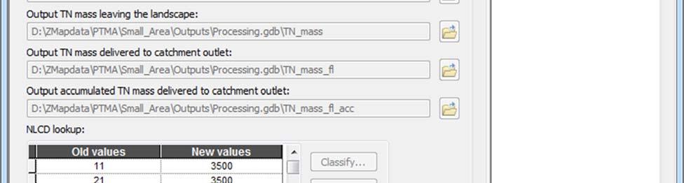
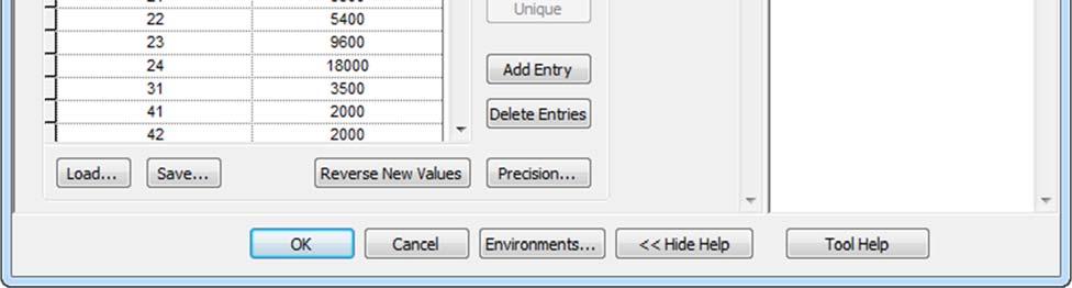
44 TOTAL NITROGEN LOADS AND ROUTING TO CATCHMENT OUTLET This tool calculates a predicted TN load leaving the landscape based on land use and literature values (see PTMApp theory and technical documentation for details) and the amount of that load reaching downstream locations. a. Inputs: i. Travel time to catchment outlet: Travel times for each raster cell to the nearest downstream catchment outlet. ii. Overland decay coefficient: The routing coefficient used in a 1 st -order decay equation to predict the sediment lost in transport during overland transport to the channelized streams. The default value for this input is 0.1. iii. Flow Direction Raster: A raster of flow direction from each cell to its steepest downslope neighbor. This layer is created outside of PTMApp preferably from a hydrologically conditioned DEM. iv. National land cover dataset: The recent data set raster whose integer values represent the land cover type. v. NLCD lookup: A lookup table relating the NLCD integer code value to a literature based annual loading value. The lookup values are multiplied by 1,000 for proper conversion within the tool (1 kg/hectare/year is entered as 1,000). b. Outputs: vi. Output TN mass Leaving the landscape: The amount of TN mass generated from the raster cell based on the land use and literature values. Units are in pounds/acre/year. vii. Output TN mass delivered to catchment outlet: The TN mass multiplied by a delivery ratio based on overland travel time to the catchment outlet. viii. Output accumulated TN mass delivered to catchment outlet: The TN mass delivered to the catchment outlet and accumulated in the downstream direction.

45 45

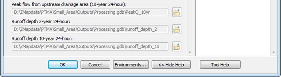
46 RUNOFF VOLUME AND PEAK FLOW In this step, PTMApp calculates the runoff volume and peak discharge for 2-year, 24-hour and 10-year, 24-hour precipitation events. The user has the option to manually change the precipitation depth of the rainfall events. a. Inputs: i. Data output folder: location where output products will be saved. ii. Flow Direction Raster: A raster of flow direction from each cell to its steepest downslope neighbor. This layer is created outside of PTMApp preferably from a hydrologically conditioned DEM. iii. Flow Accumulation Raster: A raster of accumulated flow into each cell. This layer is created outside of PTMApp preferably from a hydrologically conditioned DEM. iv. Curve Number: A Curve Number raster developed outside of the PTMApp. v. Upstream Travel Time: A raster of travel time in the upstream direction. b. Outputs: i. Catchment Runoff volume (2-year 24-hour): The catchment runoff volume in cubic feet for 2-year 24-hour rainfall event ii. Catchment Runoff volume (10-year 24-hour): The catchment runoff volume in cubic feet for 10-year 24-hour rainfall event iii. Peak flow from upstream drainage area (2-year 24-hour): Catchment peak discharge in cubic feet per second for 2-year 24-hour rainfall event iv. Peak flow from upstream drainage area (10-year 24-hour): Catchment peak discharge in cubic feet per second for 10-year 24-hour rainfall event v. Runoff depth (2-year 24-hour): Catchment runoff depth in inches for 2-year 24- hour rainfall event vi. Runoff depth (10-year 24-hour): Catchment runoff depth in inches for 10-year 24-hour rainfall event

47 47

48 SUMMARIZE CATCHMENT LOADINGS The Summarize Catchment Loading tool generates an output table that contains the source assessment information, routed to the catchment outlet, for the intervening drainage area of each unique catchment. a. Inputs: i. Data Output Folder: location where output products will be saved. ii. PTMApp products process internally include: Catchments, Sed_mass, Sed_mass_fl, Sed_mas_fl_acc, TP_mass, TP_mass_fl, TP_mas_fl_acc, TN_mass, TN_mass_fl, TN_mas_fl_acc b. Outputs: i. table_catchment: stores sediment, TP, and TN loads/yields routed to the catchment outlet

49 SEDIMENT, TOTAL PHOSPHORUS AND TOTAL NITROGEN CHANNEL ROUTING This tool calculates the amount of sediment, TP and TN load that is routed downstream based on a 1 st order decay equation using travel time. a. Inputs: i. Processing options: You may choose to determine loads/yields for priority resource catchments, adjoint catchments, or both (represented by the input All ). This option should match the option chosen when you generated your catchments. The default for this input is All. ii. Data Output Folder: location where output products will be saved. iii. Sediment channel transport coefficient: The routing coefficient used in a 1 st - order decay equation to predict the sediment lost in transport through channelized streams prior to or between priority resource points. The default value for this input is 0.2. iv. TP and TN channel decay coefficient: The routing coefficient used in a 1 st - order decay equation to predict the TP and TN lost in transport through channelized streams prior to or between priority resource points. The same value is applied for both TP and TN routing. The default value for this input is 0.1. v. Median sediment diameter: median diameter (mm) of eroded sediment. The default value for this input is 0.1. b. Outputs: i. Table catchment: Stores the leaving the landscape and delivered to catchment outlet sediment, TP and TN loading values for each catchment. ii. Adjoint Catchment Tables: Store the sediment, TP and TN loads routed to each adjoint catchment outlet (table_adj_catchment and table_adj_catchment_route). iii. Priority Resource Catchment Tables: Store the sediment, TP and TN loads routed to each priority resource outlet (table_p_res_catchment and table_p_res_catchment_route).

50 SCALED LOADS This tool is an optional tool. It scales the sediment, TP and TN loading values generated within PTMApp to match either modeled output or observed data, which may come from a calibrated watershed model or estimated loads based on monitoring data: a. Inputs:

51 51 i. Data output folder: This is the output path where the standardized PTMApp desktop geodatabases and associated data will be saved. Users can change this file path in the settings button. ii. Scale type: Select the type of data for the scaling. The model type will allow polygon features to be used for load scaling. The point type will scale loads based on observed data at one location. iii. Processing type: Select Adjoint Catchments or Proresource Catchments to run iv. the scale loads on. Spatial data layer: Choose the polygon or point feature class that contain the correct attributes. 1. The polygon layer for the Model type must be attributed with sed_yld_model, tp_yld_model, and tn_yld_model fields. 2. The point layer for the Gauge type must be attributed with sed_gauge, tp_gauge and tn_gague fields. b. Outputs: i. Table scaled load: Stores the scaled loads for sediment, TP and TN for each catchment.

52 BUILD LAKES DATA The Build Lakes Data tool uses an input lakes polygon layer to build the attribute catalog necessary to run lakes routing. This tool can be run for any storage feature provided in the lakes polygon layer, including lakes, reserviors, wetlands, and sloughs. a. Inputs: i. Data Output Folder: location where output products will be saved. ii. Lakes layer: A feature class including lake polygons which will be run through lake routing. The feature class must include the following attributes LAKE_ID (long integer) - a unique identifier for each lake Area_ac (floating point) surface area of the lake (acres) iii. Annual runoff depth: Feature class with the annual runoff depth (inches/year) summarized at a HUC-8 scale. This data is available for Minnesota in the Base.gdb. iv. Sediment channel transport coefficient: The routing coefficient used in a 1 st -order decay equation to predict the sediment lost in transport through channelized streams prior to or between priority resource points. The default value for this input is 0.2. v. TP and TN channel decay coefficient: The routing coefficient used in a 1 st -order decay equation to predict the TP and TN lost in transport through channelized streams prior to or between priority resource points. The same value is applied for both TP and TN routing. The default value for this input is 0.1. vi. Median sediment diameter: median diameter (mm) of eroded sediment. The default value for this input is 0.1. b. Outputs: i. Lakes_route: attributes were added to the Lake_route feature class in your Processing.gdb. A full description of these attributes can be found in the Attribute Catalog.

53 LAKE ROUTING The Lake Routing tool uses the sediment, TP, and TN retention fractions estimated in Build Lakes Data based on the morphometric features of each lake basin to estimate the sediment and nutrient load retained in each lake. The Build Lakes Data tool MUST be run prior to running the Lake Routing tool. a. Inputs: i. Data Output Folder: location where output products will be saved. ii. Lakes layer: The lakes layer modified in Build Lakes Data. iii. Priority resource snap point: This value determines the number of cells around each priority resource point to search for the highest flow accumulation cell. This input is necessary as priority resource points may not always be placed directly over the flow line. The default value is 0. Please reference section in

54 54 iv. Workshop Session 1 for setting this value while running Lake routing. A lower value may be recommended if lakes were conditioned using the Breakthrough method to capture lake inlets (pages in Workshop Session 1). For most applications values 0 to 5 are suitable. Data has been scaled by gauge or model (optional): optional input that should be checked if data has been scaled and you wish to have it reflected in your lake modeling results a. Outputs: i. Table priority resource catchment route: table summarizing load/yield delivered to each priority resource catchment outlet. This table will be updated based on lake routing results STREAM POWER INDEX (SPI) CALCULATOR The SPI Calculator uses rasters derived from a conditioned DEM to compute the Stream Power Index (SPI) expressed as: ln ( ). The SPI raster excludes cells with a upstream flow length less than 300 feet and cells with a larger drainage area than specified in the tool setting.

55 55 a. Inputs: i. Data output folder: location where output products will be saved. ii. Flow Accumulation Raster: A raster of accumulated flow into each cell. This layer is created outside of PTMApp preferably from a hydrologically conditioned DEM. iii. Slope raster: The slope (in percent) of the raw DEM. Only the raw DEM is required as input in this tool. iv. Upstream flow length (meters): Derived from the conditioned DEM using the spatial analyst Flow Length command with the upstream option selected. The units are meters. v. In-channel flow threshold (acres): The value defines the transistion between shallow concentrated flow and channelized flow using the cell count in the flow accumulation raster. The default value is 124. b. Outputs: i. SPI output raster: The output SPI raster.

56 MODULE: RANKING This Module allows the user to rank all of the TP, TN, and sediment loading and delivery data generated in the Catchments and Loading Module (see section 4.2) RANK - SPI This tool assigns a percentile ranking to each value in the SPI raster based on an assumed distribution. a. Input:

57 57 i. Data output folder: location where output products will be saved. ii. Catchment layer: Defines the area to assign SPI based rank values. iii. SPI raster: The input SPI raster for developing rank values that were created during the previous step. b. Output: i. SPI rank output: Raster with ranks assigned based on the input SPI raster.

58 RANK - LEAVING THE LANDSCAPE This tool assigns percentile rank values for the Sediment, TP and TN leaving the landscape loading raster using an assumed distribution. a. Inputs: ii. Data output folder: This is the output path where the standardized PTMApp desktop geodatabases and associated data will be saved. Users can change this file path in the settings button. iii. Sediment loading leaving the landscape: The amount of sediment load leaving the landscape predicted by RUSLE. iv. TN loading leaving the landscape: The TN mass leaving the landscape v. TP loading leaving the landscape: The TP mass leaving the landscape. b. Outputs: vi. Sediment ranking leaving the landscape: A raster with the percentile ranking values assigned using the assumed distribution from the sediment loading. vii. TN ranking leaving the landscape: A raster with the percentile ranking values assigned using the assumed distribution from the TN loading. viii. TP ranking leaving the landscape: A raster with the percentile ranking values assigned using the assumed distribution from the TP loading. ix. WQI mass rank: A raster combining the sediment, TP and TN ranking values with the following equation (WQI is a Water Quality Index): 0.25 _ 0.25 _ 0.5 _

59 RANK DELIVERED TO THE CATCHMENT OUTLET This tool assigns percentile rank values for the Sediment, TP and TN delivered to catchment outlet loading raster using an assumed distribution. a. Inputs: i. Data output folder: This is the output path where the standardized PTMApp desktop geodatabases and associated data will be saved. Users can change this file path in the settings button. ii. Sediment loading delivered to catchment outlet: The amount of sediment load delivered to the catchment outlet predicted by RUSLE and overland delivery ratio. iii. TN loading delivered to catchment outlet: The TN mass delivered to the catchment outlet.

60 60 iv. TP loading delivered to catchment outlet: The TP mass delivered to the catchment outlet. b. Outputs: i. Sediment ranking delivered to catchment outlet: A raster with the percentile ranking values assigned using the assumed distribution from the sediment loading. ii. TN ranking delivered to catchment outlet: A raster with the percentile ranking values assigned using the assumed distribution from the TN loading. iii. TP ranking delivered to catchment outlet: A raster with the percentile ranking values assigned using the assumed distribution from the TP loading. iv. WQI mass rank: A raster combining the sediment, TP and TN ranking values with the following equation: 0.25 _ 0.25 _ 0.5 _

61 RANK - PRIORITY RESOURCE DELIVERY This tool assigns percentile rankings to catchments based on their contribution to overall loads delivered to priority resources. a. Inputs: i. Data output folder: This is the output path where the standardized PTMApp desktop geodatabases and associated data will be saved. Users can change this file path in the settings button. b. Outputs: i. Table rank catchment: Stores percentile rankings based on a catchments unit yield of sediment, TP and TN for both leaving the landscape and delivered to catchment outlet for the entire project area. ii. Table rank priority resource catchment: Stores percentile rankings based on a catchments unit yield of sediment, TP and TN delivered to each priority resource.

62 CUSTOM WEIGHTING This tool is an optional tool. It modifies the catchment percentile rankings based on a user specified weight value. a. Inputs: i. Data output folder: This is the output path where the standardized PTMApp desktop geodatabases and associated data will be saved. Users can change this file path in the settings button. ii. Catchment: The catchment layer created in Generate Catchments. iii. User rank weight: A polygon feature class properly attributed with a rank_value field with values between 0-1. b. Outputs: i. Table r p res catchment: Appends modified ranking values to the table based on the user specified values.

63 MODULE: BEST MANAGEMENT PRACTICE (BMP) SUITABILITY This Module allows the user to identify potential locations on the landscape for the placement of BMPs and Conservation Practice (CP). In addition, the user can exclude areas for potential BMP placement based on local knowledge BMP SUITABILITY This tool uses topographic and land use characteristics and typical placement and design criteria for Best Management and Conservation Practices to locate suitable areas. Practices are categorized into treatment type categories and can be ran simultaneously or separately using the check boxes. a. Inputs: i. Data output folder: Data output folder: This is the output path where the standardized PTMApp desktop geodatabases and associated data will be saved. Users can change this file path in the settings button. ii. Treatment group check boxes (Run: storage, filtration, biofiltration, infiltration, protection, and source load reduction): Check each of the treatment groups you wish to have BMPs created for. By default, all treatment groups are checked. iii. Minimum fill depth of depression (in meters): A depressional area must have a depth greater than the minimum fill depth value to be considered suitable for storage BMPs. The default value is meters (6 inches). iv. Minimum surface area of depression (in acres): A depressional area must have a surface area greater than the minimum surface area value to be considered suitable for storage BMPs. The default value is 1 acre. b. Outputs: i. Data output folder: Separate feature classes are created for each treatment group in the assigned output folder.

64 EXCLUDED AREAS This is an optional tool which excludes areas from the BMP suitability results based on user-specified areas. This tool can be run on treatment types simultaneously or separately using the check boxes. a. Inputs: i. Data output folder: location where output products will be saved. ii. BMP null: A polygon feature class properly attributed with a bmp_group value of 0. iii. Treatment group check boxes (storage, filtration, biofiltration, infiltration, protection, and source reduction): Select the specific treatment groups you wish to have excluded. By default, all treatment groups are checked. b. Outputs i. Data output folder: Updates feature classes for each treatment type initially created in the BMP suitability tool.

65 65

66 MODULE: BENEFITS ANALYSIS This Module allows the user to estimate the efficiency of potential BMPs, calculate load reductions from BMPs at the BMP and downstream priority resources, scale load reductions based upon modeling or gage data, and conduct a treatment train analysis REDUCTION RATIO This tool estimates the ratio of water treatment to water delivered to potential BMPS and CPs. Reduction Ratio automatically finds the required inputs for completing the calculations after previous tools have been run. The tool will process even if only a subset of BMP treatment categories are present. However, if treatment categories are missing a warning will be generated in the geoprocessing results, notifying the user of the categories that were not processed. The output is the addition of data to the BMP Suitability attribute tables. The Reduction Ratio tool is sensitive to schema locks and fails to complete in case it detects such a lock see instructions under GENERAL INFORMATION on page 5. a. Inputs: i. Data output folder: This is the output path where the standardized PTMApp desktop geodatabases and associated data will be saved. Users can change this file path in the settings button. ii. Enter manual depth (optional) Use your custom 2yr and 10yr depths instead of the raster values (check if entering your own values). iii. 2yr depth: Optional depth to enter. iv. 10yr depth: Optional depth to enter.

67 67 b. Outputs: i. Various fields in the BMP treatment group feature classes are populated. Please see the Data and Attribute Catalogs for a full list of updated attributes SCREEN BMPS This tool allows the user to screen BMPs that are either too small or too inefficient to include. The input is the output from Reduction Ratio, which the tool automatically locates/accesses after the Reduction Ratio analysis has been performed. The user has the option to select which BMP Suitability Treatment Groups will be screened. The output is screened BMP Suitability datasets. Caution the Screen BMPs tool overwrites the original BMP Suitability outputs, while maintaining the attributes of those BMPs that are retained.

68 68 1. Inputs: a. Data output folder: location where output products will be saved b. BMP Treatment Group Expressions: (storage, filtration, biofiltration, infiltration, protection, and source load reduction): Query out BMPs which fall below size requirements for treating a particular design storm. Default values are based on the 10-yr, 24-hr design storm runoff. 2. Outputs: a. BMPs removed from existing treatment group feature classes.

69 REDUCTION EFFICIENCY The Reduction Efficiency tool utilizes the Reduction Ratio outputs to estimate the percent effectiveness of each potential BMP for treating TP, TN, and sediment. The Input for this tool is the BMP suitability output that has been processed through Reduction Ratio. The output from Reduction Efficiency is the percent reduction in TP, TN, and sediment attached to the BMP Suitability output attribute table for both the 2-yr, 24-hr and 10-yr, 24-hr runoff events. 2 year and 10 year, 24 hour events. 1. Inputs: a. Data output folder: location where output products will be saved b. Treatment Table: the tool internally accesses and uses table_treat in the Base.gdb in your output folder. This table, also called the Treatment Table, lists the removal efficiency statistics (including minimum, maximum, 1 st quartile, 2 nd quartile (a.k.a. median), and 3 rd quartile removal potentials for sediment, TP, and TN) for each BMP treatment group. This table will be used to estimate the removal efficiencies of BMPs in PTMApp. 2. Outputs: a. Various fields in the BMP treatment group feature classes are populated. Please see the Data and Attribute Catalogs for a full list of updated attributes. Note: The treatment table (table_treat) was developed based on an analysis of event-based BMP efficiencies aggregated in the Water Environment Research Foundation (WERF) BMP database. You may wish to update the statistics in this table to better reflect BMP efficiencies estimated in your project area or as better data becomes available.

70 70

71 ESTIMATE LOAD REDUCTIONS This tool uses the Reduction Efficiency outputs as an input and estimates TP, TN, and sediment load reductions provided by BMPs to the outlets of catchments. These calculations are performed for both the 2-yr, 24-hr and 10-yr, 24-hr runoff events. 1. Inputs: a. Data output folder: location where output products will be saved 2. Outputs: a. Various fields in the BMP treatment group feature classes are populated. Please see the Data and Attribute Catalogs for a full list of updated attributes.

72 SCALE LOAD REDUCTIONS This is an optional tool that will scale the load reductions to the catchment outlets provided by potential BMPs. The input table for scaling loads was generated in Catchments and Loading > Scale Loads and will be automatically found after that tool has been run. Note you are strongly encouraged to run this tool, if Scale Loads was run in the Catchments and Loading module to ensure load reduction outputs are consistent with your Source Assessment outputs. a. Inputs: i. Data output folder: location where output products will be saved. ii. Table scaled load: look-up table used to scale loads based on monitoring or model results. This was an output from the Catchments and Loading >> Scale Loads tool. b. Outputs: i. Various fields in the BMP treatment group feature classes are populated. Please see the Data and Attribute Catalogs for a full list of updated attributes

73 TREATMENT TRAINS This tool allows the user to estimate the load reductions in TN, TP, and sediment by BMPs that may be providing treatment in sequence. The user inputs one shapefile that has each record attributed with a treatment group code. The load reductions of the treatment train of BMPs are estimated relative to the priority resource points. Note This tool is the suggested method for estimating load reductions for a targeted implementation plan. The results will provide load reduction estimates at each priority resource point based upon the input BMP layer. a. Inputs: i. Data output folder: location where output products will be saved. ii. User BMP Path: User-created shapefile which includes all BMPs to run through the Treatment Trains procedures. This shapefile can include BMPs from multiples treatment groups. iii. Data has been scaled by gauge or model: Optional input that should be selected when PTMApp data has been scaled through Catchment and Loadings >> Scaled Data and Benefits Analysis >> Scaled Load Reductions tools. iv. Apply lakes: Optional input that should be selected when Catchments and Loading >> Lake Routing has been run and the user wished to include the effect of lakes on BMP sediment, TN, and TP reduction (at the priority resource catchment scale). b. Outputs: v. Table treat train catch: table listing results of the treatment train analysis with loads relative to the catchment outlet. vi. Table treat train priority resource: table listing results of the treatment train analysis with loads relative to the priority resource catchment outlet.

74 The input file needs to contain the outputs fields from the previous steps in the Benefits Analysis module. In other words, your input file structure should mirror the format of the BMP Suitability analysis treatment groups. 74

75 GENERATE BENEFITS TABLES This tool uses the results of Estimate Load Reductions to generate output tables from the Benefits Analysis Module that can be used for subsequent processes and generating output tables for local reporting. This tool also calculates the BMP load reductions to the priority resource points. a. Inputs: i. Data output folder: location where output products will be saved. ii. Apply lakes: Optional input that should be selected when Catchments and Loading >> Lake Routing has been run and the user wishes to include the effect of lakes on BMP sediment, TN, and TP reduction (at the priority resource catchment scale). b. Outputs: i. Table ba bmp all: table listing results of the benefits analysis. ii. Table ba load red: table listing BMP load reductions at the resource of concern. Note: Please see the Data Catalog, Attribute Catalog, and Workshop Session 3 for information on how these output tables can be used.

76 ATTACH TO CATCHMENTS This tool attaches the outputs from Benefits Analysis to the Catchment databases and prepares the data for use in the Cost Analysis Module. The output from this tool is needed to run tools in the Cost Analysis Module. a. Inputs: i. Data output folder: location where output products will be saved. b. Outputs: i. Table ba bmp all catchment: table showing one set of values per BMP treatment group for each catchment.

77 MODULE: COST ANALYSIS This module estimates the treatment cost ($/mass reduced) for potential BMPs based upon the default Minnesota EQUIP payment schedule on a per unit basis. The user has the option to adjust the per unit cost estimates based upon local knowledge. a. Inputs: i. Data output folder: location where output products will be saved. ii. Table ba bmp all catchment: table created in the previous tool, Benefits Analysis >> Attached to Catchments, the table lists one set of values per BMP treatment group for each catchment. iii. Units costs for BMP treatment groups. Default values are shown below and should be adjusted based on local knowledge: Storage Cost: $0.10 per cubic-yard Filtration Cost: $ per acre Biofiltration Cost: $44.92 per cubic-yard Infiltration Cost: $27, per acre (or ~ $5.62/sq-yard) Protection Cost: $2, per acre Source Reduction Cost: $30.87 per acre Note: We strongly recommend you review and update (if necessary) these costs to ensure they reflect costs of BMP installations in your area. b. Outputs: i. Table ca bmp costeff: Table with BMP cost effectiveness

78 78

79 EXTRACT FOR WEB This tool formats and packages data into a zip file for use in the PTMApp website. a. Inputs: i. Input processing geodatabase: This is the output path where the standardized PTMApp desktop geodatabases and associated data will be saved. Users can change this file path in the settings button. ii. Output location: Folder where the output zip file will be written. iii. Name your upload data: Name given to all files within the output. iv. Select on watershed one plan: Select your watershed from a dropdown list of all Minnesota 1W1P watersheds. v. Create name: Name of person creating this output zip. vi. Quality control output path: Location were QC text file will be created vii. Quality control file name: Name of QC text file.