June 2018 WORKSHOP SECTION 2 MANUAL: RUNNING PTMAPP-DESKTOP AN INNOVATIVE SOLUTION BY:

Transcription

1 June 2018 WORKSHOP SECTION 2 MANUAL: RUNNING PTMAPP-DESKTOP AN INNOVATIVE SOLUTION BY:

2 TABLE OF CONTENTS 1 PURPOSE SET UP DATA PATHS BASE DATA SETUP INGEST DATA CLIP WATERSHED PREPROCESSING CATCHMENTS AND LOADING GENERATE CATCHMENTS RUSLE CALCULATOR TRAVEL TIME TO CATCHMENT OUTLET SEDIMENT DELIVERY RATIO TO CATCHMENT OUTLET SEDIMENT ROUTING TO CATCHMENT OUTLET TOTAL PHOSPHORUS LOADS AND ROUTING TO CATCHMENT OUTLET TOTAL NITROGEN LOADS AND ROUTING TO CATCHMENT OUTLET RUNOFF VOLUME AND PEAK FLOW SUMMARIZE CATCHMENT LOADINGS SEDIMENT, TOTAL PHOSPHORUS AND TOTAL NITROGEN CHANNEL ROUTING: SCALED LOADS BUILD LAKES DATA LAKE ROUTING STREAM POWER INDEX (SPI) CALCULATOR RANKING SPI RANK LEAVING THE LANDSCAPE DELIVERED TO THE CATCHMENT OUTLET PRIORITY RESOURCE DELIVERY CUSTOM WEIGHTING BEST MANAGEMENT PRACTICE (BMP) SUITABILITY BMP SUITABILITY EXCLUDED AREAS INGEST ACPF BENEFITS ANALYSIS REDUCTION RATIO SCREEN BMPS REDUCTION EFFICIENCY ESTIMATE LOAD REDUCTIONS SCALE LOAD REDUCTIONS

3 7.6 TREATMENT TRAINS PREPROCESS TREATMENT TRAINS GENERATE BENEFITS TABLES ATTACH TO CATCHMENTS COST ANALYSIS COST ANALYSIS EXTRACT FOR WEB EXTRACT FOR WEB

4 1 PURPOSE The Prioritize, Target, Measure Application (PTMApp) is a software solution that consists of PTMApp-Desktop (an ArcGIS toolbar) and PTMApp-Web (Website) to assist practitioners with executing their strategies. This workshop manual provides instructions for setup and use of PTMApp-Desktop. The contents of this manual assume that the user has reviewed the full PTMApp-Desktop User Guide or taken the PTMApp-Desktop Workshop on preparing inputs for the toolbar. It also assumes that PTMApp-Desktop has already been installed on the user s computer (see PTMApp-Desktop User Guide for installation instructions). PTMApp-Desktop is a collection of tools developed to create a suite of Geographic Information System (GIS) products. The toolbar is organized into a series of modules which create a set of GIS products used in subsequent modules. The toolbar is distributed with base GIS data which can be clipped to your specific planning boundary. The products developed using the PTMApp-Desktop toolbar are intended to be used in the development of One Watershed - One Plan, source assessment, developing implementation plans, and assessing the ability to achieve various load reductions for sediment, nitrogen and phosphorus. ****Note**** this manual assumes the user has at least introductory experience using ArcGIS. Users should be familiar with adding data to a map project, joining data tables, formatting map symbology, querying data based on attributes, and spatial selection. It also assumes that the user is familiar with preparing input data for PTMApp-Desktop and processing data through the toolbar. User s should be aware the ESRI ArcGIS products tend to place read-write protection, also called schema locks, on data products that are opened within the software. Using the toolbar relies heavily upon retaining the rights to read and write data. As such, is recommended that users avoid opening data within ArcGIS or other programs while performing operations in the toolbar. If an error does occur, the user will need to close all ArcGIS software, exit out of any other software where data was being viewed, and restart ArcGIS. 3

5 2 SET UP DATA PATHS 2.1 BASE DATA SETUP Description - The toolbar is distributed with a state-wide (Minnesota) geodatabase called Base.gdb. The geodatabase contains many different types of GIS data useful in completing watershed plans, understanding water movement and for characterizing watershed conditions. Steps HOW TO: 1. Place this file geodatabase on your local computer or system network in a preferred location. Then, click the settings tab on the toolbar. 2. Specify the path to the Base.gdb here. 3. The Base.gdb data as well as some planning and processing data provided by the user, must be clipped to your watershed for analysis. All output data will be stored in geodatabases created in the workspace you assign here. Specify that workspace path here. Click Ok to save changes. 4

6 5 4. These will be your default settings for the toolbar (If you want to run a different watershed with different paths this can be done). Click the Send Error Logs string in the left window below and you will see a path to ing an error log. The default is ptmapp@state.mn.us. If an error occurs during processing you can forward an error log to the PTMApp Development Team at this . The error log is a text file named ERROR_LOG.txt. The information in this log is helpful for the developers when debugging the error. This error text file is generated once Clip Watershed is run and updated as any additional errors are generated while running PTMApp-Desktop.

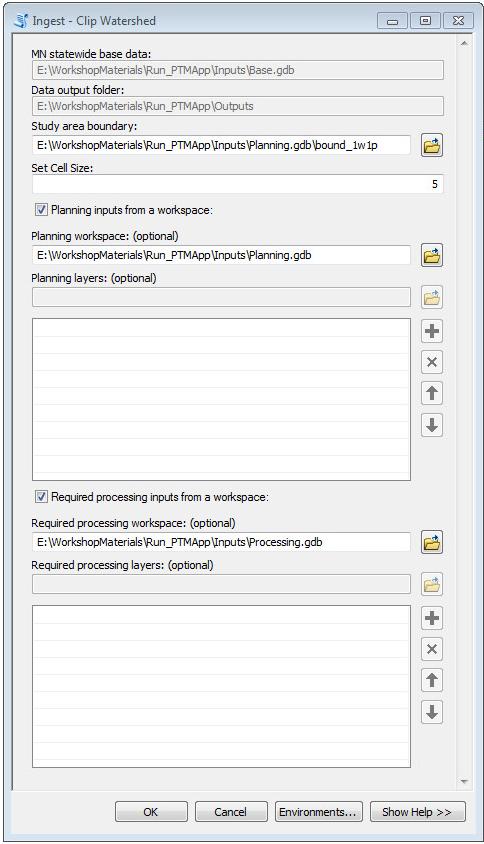
7 5. To save your settings, click either OK or Apply 3 INGEST DATA The Ingest Data Module is the starting point for processing data using PTMApp-Desktop. This module allows the user to set their analysis study area, clip the base data to their study area, and complete pre-processing necessary to run the remainder of the Modules. The study area file must be created prior to this step as a required input for PTMApp-Desktop. 3.1 CLIP WATERSHED Description - Clip Watershed confirms that all files needed to run PTMApp-Desktop are present and clips them to the extent of your study area (study area = bound_1w1p). Users have the option to drag and drop individual files or input their entire workspace. We suggest the following structure for the required processing workspace (called processing.gdb here) and planning workspace (called planning.gdb). We recommend using this structure as the same structure will be created in your output files. 6

8 Steps 1. On the PTMApp-Desktop toolbar go to Ingest Data - > Clip Watershed 2. The window below will appear. Specify the watershed to clip all the layers to in the Study area boundary parameter. Set Cell Size based on the cell size of your input rasters (in our workshop example, 5 meters). Input data (e.g. Planning and Processing file geodatabases) into the rest of the parameters for clipping the base, planning, and processing map data. After this tool, the processing can begin. 7

9 8

10 3. Upon completion, a text file is created indicating any missing layers needed for other PTMApp- Desktop modules. Clip Watershed now also includes functionality to check inputs provided by the user to ensure data meets formatting requirements of PTMApp-Desktop and is within expected bounds for data gathered in the State of 9

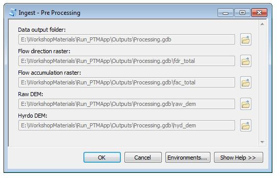
11 Minnesota. A list of these checks is provided in the Download QA/QC Desktop Outputs document on the PTMApp-Desktop/Theory & Documentation website. 3.2 PREPROCESSING DESCRIPTION - In this step, the remainder of preprocessing data needed for subsequent modules will be generated. After successfully running Clip Watersheds, the Preprocessing tool will automatically find all required inputs. Steps 1. Inputs: a. Data output folder: This is the output path where the standardized PTMApp-Desktop geodatabases and associated data will be saved. Users can change this file path in the settings button. b. Flow direction raster (fdr_total OR fdr_surf): A raster of flow direction from each cell to its steepest downslope neighbor. This layer is created outside of PTMApp-Desktop (preferably from a hydrologically-conditioned DEM). Guidance on creating this input has been provided as part of Workshop Section 1 in this 3-part workshop series. c. Flow accumulation raster (fac_total OR fac_surf): A raster of accumulated flow into each cell. This layer is created outside of PTMApp-Desktop (preferably from a hydrologicallyconditioned DEM). d. Raw DEM (raw_dem): The raw elevation DEM. e. Hydrologically-Conditioned DEM (hyd_dem): The raw elevation DEM modified to account for sub-surface flow paths and non-contributing areas (if included in analysis). 10

12 11

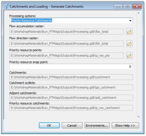
13 4 CATCHMENTS AND LOADING The Catchments and Loading module generates the fields scale catchments, estimates TN, TP, and sediment loads and yields both leaving the landscape and delivered to downstream priority resources, generates the stream power index (SPI), and performs volume and peak discharge calculations. This module also provides the user the opportunity to scale source loading data based on model (HSPF or SWAT) or monitoring data. 4.1 GENERATE CATCHMENTS DESCRIPTION - The Generate Catchments tool divides the planning area into catchments averaging approximately 40 acres in size, creates overlapping adjoint catchments that vary in size (if chosen) and priority resource catchments (if chosen) containing the watershed area for input priority resource outlet points. Steps 12

14 1. Inputs: a. Processing Options: You may choose to generate priority resource catchments, adjoint catchments, or both (represented by the input All ). New catchments will be created (or recreated if running again) for any of the three options available. The default for this input is All. Priority Resource Catchments are used to summarize flow to a resource point and should be chosen for this workshop. b. Flow Accumulation Raster: A raster of accumulated flow into each cell. This layer is created outside of PTMApp-Desktop (preferably from a hydrologically-conditioned DEM). c. Flow Direction Raster: A raster of flow direction from each cell to its steepest downslope neighbor. This layer is created outside of PTMApp-Desktop (preferably from a hydrologicallyconditioned DEM). d. Priority Resource Points: locations of priority resource points which will be used to delineate priority resource catchments e. Priority Resource Snap Point: This value determines the number of cells around each priority resource point to search for the highest flow accumulation cell. This input is necessary as priority resource points may not always be placed directly over the flow line. The default value is 0. Please reference section in Workshop Session 1 for setting this value while running Lake routing. A lower value may be recommended if lakes were conditioned using the Breakthrough method to capture lake inlets (pages in Workshop Section 1). Please not that using a snap point of 0 WILL require you to place the resource point directly on the fac_total or fac_surf flowline. You may wish to increase this value if your points may not fall directly on the flowline. Values up to 5 are common. 2. Outputs: a. Catchments: Subwatershed polygons delineated from the flow direction raster ranging in size from acres (40 acres on average) covering the entire planning boundary. b. Catchment Outlets: Raster layer with unique IDs corresponding to the catchments, adjoint catchments, and priority resource catchments. 1. ID values less than 9,900 are priority resource catchments 2. ID values between 9,900 and 500,000 are adjoint catchments 3. ID values greater than 500,000 are catchments. c. Adjoint Catchments: Watershed polygons delineated from the flow direction raster for all non-headwater catchments. Each watershed polygon encompasses the entire upstream drainage area for the corresponding pour point. d. Priority Resource Catchments: Watershed polygons delineated from the flow direction raster for all priority resource pour points imported in the Planning geodatabase. 13

15 14

16 4.2 RUSLE CALCULATOR Description - The RUSLE Calculator uses methodology and processes described in the USDA-ARS Agricultural Handbook No. 703 to compute an estimated annual sediment load leaving the landscape. Steps 1. Inputs: a. Raw elevation raster: The raw elevation DEM. b. Input Raw raster Z factor: Multiplies the elevation values by this factor. Default value is 1. c. Input R Factor: The Rainfall-Runoff Erosivity Factor (R) must have the same cell size as the raw DEM and have floating point values. d. Input Kw Factor: The Soil Erodibility Factor (Kw) is the soil-loss rate per erosion index unit for a specified soil as measured on a standard plot. The factor is available from the SSURGO soils database and should be a floating point raster with a cell size matching the raw DEM. e. Input C Factor: The Cover-Management Factor (C) is a ratio of soil loss from an area with specified cover and management to soil loss from an identical area in tilled continuous fallow. The C Factor is derived from the NASS dataset. It should have a cell size matching the raw DEM and have floating point values. f. Input P Factor: The Support Practice Factor (P Factor) is the ratio of soil loss with a support practice like contouring, stripcropping, or terracing to soil loss with straight-row farming up and down the slope. The P Factor should contain floating point values (but can be integer if all values equal 1) and have a cell size matching the raw DEM. g. M Weight Factor: Used in calculating of the Length-Slope Factor (LS). The M-weight factor allows for variation in the ratio of rill to Inter-rill erosion. This factor should also contain floating 15

17 point values (but can be integer if all values equal 1) and have a cell size matching the raw DEM. h. Input Upstream Flow Length: Derived from the conditioned DEM using the spatial analyst Flow Length command with the upstream option selected. The units are meters if Workshop Session 1 guidance was followed. i. Flow Direction Raster: A raster of flow direction from each cell to its steepest downslope neighbor. This layer is created outside of PTMApp preferably from a hydrologically-conditioned DEM. 2. Outputs: a. RUSLE sediment loss raster: The sediment loss rate predicted by RUSLE in tons/acre/year. b. Output LS Factor: Length-slope factor computed using the hydrologically-conditioned DEM. 16

18 Special Note: Messages such as the one below may appear with results for individual tools in the Ingest Data and Catchments and Loading modules to alert the users that his/her data may be out of range or not meet PTMApp-Desktop s specific input requirements. If one of these messages pop up, please review the specific data inputs/outputs it references to make sure they meet requirements of the PTMApp-Desktop tool. In some cases, these message may be erronously caused by rounding errors in ArcGIS. The message below is an example. The minimum LS -factor is actually , which was identified as < Obviously, this small difference is negligle and can be ignored. 4.3 TRAVEL TIME TO CATCHMENT OUTLET Description The Travel Time to Catchment Outlet tool computes the travel times for each raster cell to the nearest downstream catchment outlet using conditioned DEM products and a raster representing the travel time between cells. These travel times will be used to route sediment, total nitrogen (TN), and total phosphorus (TP) to the catchment outlet. 17

19 Steps 1. Inputs: a. Flow Direction Raster: A raster of flow direction from each cell to its steepest downslope neighbor. This layer is created outside of PTMApp (preferably from a hydrologicallyconditioned DEM). b. Flow Accumulation Raster: A raster of accumulated flow into each cell. This layer is created outside of PTMApp (preferably from a hydrologically-conditioned DEM). c. Time grid (in seconds) cell to cell: Raster representing the travel time between cells. 2. Outputs: a. Travel time to catchment outlet (in hours): Travel times for each raster cell to the nearest downstream catchment outlet. 18

20 4.4 SEDIMENT DELIVERY RATIO TO CATCHMENT OUTLET Description - The Overland SDR Calculator uses drainage area and flow length to calculate an overland Sediment Delivery Ratio (SDR) computed as [SDR = 0.41 x Drainage Area (in square kilometers) -0.3 ] with an additional adjustment based on the flow length distance to the flow line. Steps 1. Inputs: a. Grid cell SDR adjustment factor: Coefficient used within the Overland SDR Adjustment Factor equation to adjust the Overland SDR based on flow length. Default value is b. Flow Direction Raster: A raster of flow direction from each cell to its steepest downslope neighbor. This layer is created outside of PTMApp (preferably from a hydrologicallyconditioned DEM). c. Flow Accumulation Raster: A raster of accumulated flow into each cell. This layer is created outside of PTMApp (preferably from a hydrologically-conditioned DEM). d. Catchments: The catchment hydrologic boundaries created in the Generate Catchments tool. 2. Outputs: a. Output sediment delivery ratio: The ratio the RUSLE sediment load delivered to the catchment outlet. 19

21 4.5 SEDIMENT ROUTING TO CATCHMENT OUTLET Description The Sediment Routing to Catchment Outlet tool calculates the amount of sediment load predicted by RUSLE delivered to the catchment outlet. 20

22 Steps 1. Inputs: a. Sediment delivery ratio raster: The ratio the RUSLE sediment load delivered to the catchment outlet. b. RUSLE raster: The sediment loss rate predicted by RUSLE in tons/acre/year. c. Flow Direction Raster: A raster of flow direction from each cell to its steepest downslope neighbor. This layer is created outside of PTMApp (preferably from a hydrologicallyconditioned DEM). d. Flow Accumulation Raster: A raster of accumulated flow into each cell. This layer is created outside of PTMApp (preferably from a hydrologically-conditioned DEM). e. RUSLE adjustment factor: A multiplying factor used to calibrate the predicted sediment load by RUSLE to observed sediment load measurements. Default value is 1 (meaning no additional calibration). 2. Outputs: a. Output sediment mass Leaving the Landscape: The input sediment loss raster multipled by the RUSLE adjustment factor. Units are tons/acre/year. b. Output sediment mass delivered to catchment outlet: The amount of sediment load predicted by RUSLE delivered to the catchment outlet c. Accumulated sediment mass delivered to catchment outlet: The amount of sediment load delivered to the catchment outlet accumulated in the downstream direction. 21

23 4.6 TOTAL PHOSPHORUS LOADS AND ROUTING TO CATCHMENT OUTLET Description The Total Phosphorous Loads and Routing to Catchment Outlet tool calculates a predicted Total Phosphorus (TP) load leaving the landscape based on land use and literature values and the amount of that load reaching downstream locations. Steps 1. Inputs: a. Travel time to catchment outlet: Travel times for each raster cell to the nearest downstream catchment outlet. b. Overland decay coefficient: The routing coefficient used in a 1 st -order decay equation to predict the sediment lost in transport during overland transport to the channelized streams. The default value for this input is 0.1. c. Flow Direction Raster: A raster of flow direction from each cell to its steepest downslope neighbor. This layer is created outside of PTMApp (preferably from a hydrologicallyconditioned DEM). d. National land cover dataset: The recent data set raster whose integer values represent the land cover type. e. NLCD lookup: A lookup table relating the NLCD integer code value to a literature-based TP annual yield value. The lookup values are multiplied by 1,000 for proper conversion within the tool (i.e. 1 kg/hectare/year is entered as 1,000). 2. Outputs: a. Output TP mass Leaving the landscape: The amount of TP mass generated from the raster cell based on the land use and literature values. Units are in pounds/acre/year. b. Output TP mass delivered to catchment outlet: The TP mass multiplied by a delivery ratio based on overland travel time to the catchment outlet. 22

24 23 c. Output accumulated TP mass delivered to catchment outlet: The TP mass delivered to the catchment outlet and accumulated in the downstream direction.

25 4.7 TOTAL NITROGEN LOADS AND ROUTING TO CATCHMENT OUTLET Description The Total Nitrogen Loads and Routing to Catchment Outlet tool calculates a predicted total nitrogen (TN) load leaving the landscape based on land use and literature values and the amount of that load reaching downstream locations. Steps 1. Inputs: a. Travel time to catchment outlet: Travel times for each raster cell to the nearest downstream catchment outlet. b. Overland decay coefficient: The routing coefficient used in a 1 st -order decay equation to predict the sediment lost in transport during overland transport to the channelized streams. c. Flow Direction Raster: A raster of flow direction from each cell to its steepest downslope neighbor. This layer is created outside of PTMApp (preferably from a hydrologicallyconditioned DEM). d. National land cover dataset: The recent data set raster whose integer values represent the land cover type. e. NLCD lookup: A lookup table relating the NLCD integer code value to a literature-based TN annual yield value. The lookup values are multiplied by 1,000 for proper conversion within the tool (i.e. 1 kg/hectare/year is entered as 1,000) 2. Outputs: a. Output TN mass Leaving the landscape: The amount of TN mass generated from the raster cell based on the land use and literature values. Units are in pounds/acre/year. 24

26 25 b. Output TN mass delivered to catchment outlet: The TN mass multiplied by a delivery ratio based on overland travel time to the catchment outlet. c. Output accumulated TN mass delivered to catchment outlet: The TN mass delivered to the catchment outlet and accumulated in the downstream direction.

27 4.8 RUNOFF VOLUME AND PEAK FLOW Description The Runoff Volume and Peak Flow tool calculates the runoff volume and peak discharge for 2-year and 10-year 24-hour precipitation events. The user has the option to manually change the precipitation depth of the rainfall events. Steps 1. Inputs: a. Data Output Folder: location where output products will be saved. b. Flow Direction Raster: A raster of flow direction from each cell to its steepest downslope neighbor. This layer is created outside of PTMApp (preferably from a hydrologicallyconditioned DEM). c. Flow Accumulation Raster: A raster of accumulated flow into each cell. This layer is created outside of PTMApp (preferably from a hydrologically-conditioned DEM). d. Curve Number: A Curve Number raster developed outside of PTMApp. e. Upstream Travel Time: A raster of travel time in the upstream direction. 2. Outputs: a. Catchment Runoff volume (2-year 24-hour): The catchment runoff volume in cubic feet for 2-year 24-hour rainfall event b. Catchment Runoff volume (10-year 24-hour): The catchment runoff volume in cubic feet for 10-year 24-hour rainfall event c. Peak flow from upstream drainage area (2-year 24-hour): Catchment peak discharge in cubic feet per second for 2-year 24-hour rainfall event 26

28 27 d. Peak flow from upstream drainage area (10-year 24-hour): Catchment peak discharge in cubic feet per second for 10-year 24-hour rainfall event e. Runoff depth (2-year 24-hour): Catchment runoff depth in inches for 2-year 24-hour rainfall event f. Runoff depth (10-year 24-hour): Catchment runoff depth in inches for 10-year 24-hour rainfall event

29 4.9 SUMMARIZE CATCHMENT LOADINGS Description The Summarize Catchment Loading tool generates an output table that contains the source assessment information, routed to the catchment outlet, for the intervening drainage area of each unique catchment. Steps 1. Inputs: a. Data Output Folder: location where output products will be saved. b. PTMApp products processed internally include: Catchments, Sed_mass, Sed_mass_fl, Sed_mas_fl_acc, TP_mass, TP_mass_fl, TP_mas_fl_acc, TN_mass, TN_mass_fl, TN_mas_fl_acc 2. Outputs: a. table_catchment: stores sediment, TP, and TN loads/yields routed to the catchment outlet. 28

30 4.10 SEDIMENT, TOTAL PHOSPHORUS AND TOTAL NITROGEN CHANNEL ROUTING: Description The Sediment, TP and TN Channel Routing tool calculates the amount of sediment, TP and TN load that is routed downstream based on a 1 st -order decay equation using travel time. Steps 1. Inputs: a. Processing Options: You may choose to determine loads/yields for priority resource catchments, adjoint catchments, or both (represented by the input All ). This option should match the option chosen when you generated your catchments. The default for this input is All. b. Data Output Folder: location where output products will be saved. c. Sediment channel transport coefficient: The routing coefficient used in a 1 st -order decay equation to predict the sediment lost in transport through channelized streams prior to or between priority resource points. The default value for this input is 0.2. d. TP and TN channel decay coefficient: The routing coefficient used in a 1 st -order decay equation to predict the TP and TN lost in transport through channelized streams prior to or between priority resource points. The same value is applied for both TP and TN routing. The default value for this input is 0.1. e. Median sediment diameter: median diameter (mm) of eroded sediment. The default value for this input is

31 30 2. Outputs: a. Table catchment: Stores the leaving the landscape and delivered to catchment outlet sediment, TP and TN loading values for each catchment. b. Adjoint Catchment Tables: Store the sediment, TP and TN loads routed to each adjoint catchment outlet (table_adj_catchment and table_adj_catchment_route). c. Priority Resource Catchment Tables: Store the sediment, TP and TN loads routed to each priority resource outlet (table_p_res_catchment and table_p_res_catchment_route).

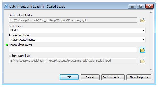
32 4.11 SCALED LOADS Description The Scaled Loads tool scales the sediment, TP and TN loading values generated within PTMApp to match either modeled output or observed data, which may come from a calibrated watershed model or estimated loads based on monitoring data. This is an optional button which should only be run if you wish to modify your loads to better match modeled or monitored data. Steps 1. Inputs: a. Data Output Folder: location where output products will be saved. b. Scale type: Select the type of data for the scaling. The model type will allow polygon features to be used for load scaling. The point type will scale loads based on observed data at one location. c. Processing type: Choose which catchment layer you would like loadings to be scale for: Adjoint Catchments or Priority Resource Catchments. d. Spatial data layer: Choose the polygon or point feature class that contain the correct attributes. 1. The polygon layer for the Model type must be attributed with sed_yld_model, tp_yld_model, and tn_yld_model fields. 2. The point layer for the Gauge type must be attributed with sed_gauge, tp_gauge and tn_gague fields. 2. Outputs: a. Table scaled load: Stores the scaled loads for sediment, TP and TN for each catchment. 31

33 32

34 4.12 BUILD LAKES DATA Description - The Build Lakes Data tool uses an input lakes polygon layer to build the attribute catalog necessary to run lakes routing. Steps 1. Inputs: a. Data Output Folder: location where output products will be saved. b. Lakes layer: A feature class including lake polygons which will be run through lake routing. The feature class must include the following attributes i. LAKE_ID (long integer) - a unique identifier for each lake ii. Area_ac (floating point) surface area of the lake (acres) c. Annual runoff depth: Feature class with the annual runoff depth (inches/year) summarized at a HUC-8 scale. This data is available for Minnesota in the Base.gdb. d. Sediment channel transport coefficient: The routing coefficient used in a 1 st -order decay equation to predict the sediment lost in transport through channelized streams prior to or between priority resource points. The default value for this input is 0.2. e. TP and TN channel decay coefficient: The routing coefficient used in a 1 st -order decay equation to predict the TP and TN lost in transport through channelized streams prior to or between priority resource points. The same value is applied for both TP and TN routing. The default value for this input is

35 f. Median sediment diameter: median diameter (mm) of eroded sediment. The default value for this input is Outputs: a. Lakes_route: attributes were added to the Lake_route feature class in your Processing.gdb. A full description of these attributes can be found in the Attribute Catalog. 34

36 4.13 LAKE ROUTING Description The Lake Routing tool uses the sediment, TP, and TN retention fractions estimated in Build Lakes Data based on the morphometric features of each lake basin to estimate the sediment and nutrient load retained in each lake. Build Lakes Data MUST be run prior to running Lake Routing. Steps 1. Inputs: a. Data Output Folder: location where output products will be saved. b. Lakes layer: The lakes layer modified in Build Lakes Data. c. Priority resource snap point: This value determines the number of cells around each priority resource point to search for the highest flow accumulation cell. This input is necessary as priority resource points may not always be placed directly over the flow line. The default value is 0. Please reference section in Workshop Session 1 for setting this value while running Lake routing. A lower value may be recommended if lakes were conditioned using the Breakthrough method to capture lake inlets (pages in Workshop Session 1). For most applications values 0 to 5 are suitable. d. Data has been scaled by gauge or model (optional): optional input that should be checked if data has been scaled and you wish to have it reflected in your lake modeling results 2. Outputs: a. Table priority resource catchment route: table summarizing load/yield delivered to each priority resource catchment outlet. This table will be updated based on Lake Routing results. 35

37 4.14 STREAM POWER INDEX (SPI) CALCULATOR Description - The SPI Calculator tool uses rasters derived from a conditioned DEM to compute the Stream Power Index (SPI) expressed as: ln ( ). The SPI raster excludes cells with an upstream flow length less than 300 feet and cells with a larger drainage area than specified in the tool setting. 36

38 Steps 1. Inputs: a. Data Output Folder: location where output products will be saved. b. Flow Accumulation Raster: A raster of accumulated flow into each cell. This layer is created outside of PTMApp (preferably from a hydrologically-conditioned DEM). c. Slope raster: The slope (in percent) of the raw DEM. e. Upstream flow length (meters): Derived from the conditioned DEM using the Spatial Analyst Flow Length command with the upstream option selected. The units are meters. f. In-channel flow threshold (acres): The value (# of cells) defines the transition between shallow concentrated flow and channelized flow using the cell count in the flow accumulation raster. The default value is Outputs: a. SPI raster: The output SPI raster. 37

39 5 RANKING The Ranking tool allows the user to rank all of the TP, TN, and sediment loading and delivery data generated in the Catchments and Loading Module. 5.1 SPI RANK Description The SPI Rank tool assigns a percentile ranking to each value in the SPI raster based on an assumed distribution. Steps 1. Input: a. Data Output Folder: location where output products will be saved. b. Catchment layer: Defines the area to assign SPI based rank values. c. SPI raster: The input SPI raster for developing rank values. 2. Output: a. SPI rank output: Raster with ranks assigned based on the input SPI raster. 38

40 5.2 LEAVING THE LANDSCAPE Description The Leaving the Landscape tool assigns percentile rank values for the Sediment, TP and TN leaving the landscape loading raster using an assumed distribution. Steps 1. Inputs: a. Data Output Folder: location where output products will be saved. a. Sediment loading leaving the landscape: The amount of sediment load leaving the landscape as predicted by RUSLE. b. TN loading leaving the landscape: The TN mass leaving the landscape. c. TP loading leaving the landscape: The TP mass leaving the landscape. 2. Outputs: a. Sediment ranking leaving the landscape: A raster with the percentile ranking values assigned using the assumed distribution from the sediment loading. b. TN ranking leaving the landscape: A raster with the percentile ranking values assigned using the assumed distribution from the TN loading. 39

41 c. TP ranking leaving the landscape: A raster with the percentile ranking values assigned using the assumed distribution from the TP loading. d. WQI mass rank: A raster combining the sediment, TP and TN ranking values with the following equation: (WQI is a Water Quality Index) 0.25 _ 0.25 _ 0.5 _ 40

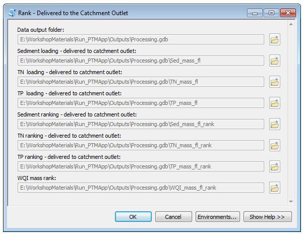
42 5.3 DELIVERED TO THE CATCHMENT OUTLET Description The Delivered to the Catchment Outlet tool assigns percentile rank values for the Sediment, TP and TN leaving the landscape loading raster using an assumed distribution. Steps 1. Inputs: a. Data output folder: location where output products will be saved. b. Sediment loading delivered to catchment outlet: The amount of sediment load delivered to the catchment outlet predicted by RUSLE and overland delivery ratio. c. TN loading delivered to catchment outlet: The TN mass delivered to the catchment outlet. d. TP loading delivered to catchment outlet: The TP mass delivered to the catchment outlet. 2. Outputs: a. Sediment ranking delivered to catchment outlet: A raster with the percentile ranking values assigned using the assumed distribution from the sediment loading. b. TN ranking delivered to catchment outlet: A raster with the percentile ranking values assigned using the assumed distribution from the TN loading. c. TP ranking delivered to catchment outlet: A raster with the percentile ranking values assigned using the assumed distribution from the TP loading. d. WQI mass rank: A raster combining the sediment, TP and TN ranking values with the following equation: 0.25 _ 0.25 _ 0.5 _ 41

43 42

44 5.4 PRIORITY RESOURCE DELIVERY Description The Priority Resource Delivery tool assigns percentile rankings to catchments based on their contribution to overall loads delivered to priority resources. Steps 1. Inputs: a. Data output folder: location where output products will be saved. 2. Outputs: a. Table rank catchment: Stores percentile rankings based on a catchments unit yield of sediment, TP and TN for both leaving the landscape and delivered to catchment outlet for the entire project area. b. Table rank priority resource catchment: Stores percentile rankings based on a catchments unit yield of sediment, TP and TN delivered to each priority resource. 43

45 5.5 CUSTOM WEIGHTING Description The Custom Weighting tool modifies the catchment percentile rankings based on a user specified weight value. This is an optional tool. Steps 1. Inputs: a. Data output folder: location where output products will be saved. b. Catchment: the catchment layer created in Generate Catchments c. User rank weight: A polygon feature class properly attributed with a rank_value field with values between Outputs: a. Table r p res catchment: Appends modified ranking values to the table based on the user specified values. 44

46 6 BEST MANAGEMENT PRACTICE (BMP) SUITABILITY This Module allows the user to identify potential locations on the landscape for the placement of BMPs and Conservation Practices (CP). In addition, the user can exclude areas for potential BMP placement based on local knowledge. 6.1 BMP SUITABILITY Description The BMP Suitability tool uses topographic and land use characteristics and typical placement and design criteria for Best Management and Conservation Practices to locate suitable areas. Practices are categorized into treatment type categories and can be ran simultaneously or separately using the check boxes. Steps 1. Inputs: a. Data output folder: location where output products will be saved. b. Treatment group check boxes (Run: storage, filtration, biofiltration, infiltration, protection, and source load reduction): Check each of the treatment groups you wish to have BMPs created for. By default, all treatment groups are checked. c. Minimum fill depth of depression (in meters): For storage, a depressional area must have a depth greater than the minimum fill depth value to be considered suitable for storage BMPs. The default value is meters (6 inches). d. Minimum surface area of depression (in acres): For storage, a depressional area must have a surface area greater than the minimum surface area value to be considered suitable for storage BMPs. The default value is 1 acre. 2. Outputs: a. Data output folder: Separate feature classes are created for each treatment group in the assigned output folder. 45

47 6.2 EXCLUDED AREAS Description The Excluded Areas tool excludes areas from the BMP suitability results based on userspecified areas. This tool can be run on treatment types simultaneously or separately using the check boxes. This is an optional tool. Steps 1. Inputs: a. Data output folder: location where output products will be saved. b. BMP null: A polygon feature class properly attributed with a bmp_group value of 0. 46

48 47 c. Treatment group check boxes (storage, filtration, biofiltration, infiltration, protection, and source reduction): Select the specific treatment groups you wish to have excluded. By default, all treatment groups are checked. 2. Outputs: a. Data output folder: Updates feature classes for each treatment type initially created in the BMP suitability tool.

49 6.3 INGEST ACPF Description This tool ingest practice polygons into PTMApp-Desktop that were identified by the Agricultural Conservation Planning Framework (ACPF) tool. Conservation practice placement opportunities mapped by the ACPF toolset include 13 different practices, including controlled drainage, grassed waterways, water and sediment control basins, and nutrient removal wetlands. The Ingest ACPF button attributes ACPF practices locations with necessary PTMApp-Desktop attributes and water quality benefits, including constituent delivery to the practices, and sediment, total phosphorus and total nitrogen removal both locally and regionally. Please note that you do not need to run Benefits Analysis or Cost Analysis for ACPF polygons run through this tool. The Ingest ACPF button runs the algorithms in the Benefits Analysis and Cost Analysis tools for you and creates each of the output products otherwise created in those modules. Steps 1. Inputs: a. Data output folder: location where output products will be saved. b. BMP null: A polygon feature class properly attributed with a bmp_group value of 0. c. Treatment group check boxes (storage, filtration, biofiltration, infiltration, protection, and source reduction): Select the specific treatment groups you wish to have excluded. By default, all treatment groups are checked. d. Input ACPF GDB: File geodatabase containing the ACPF dataset e. Output ACPF GDB: Empty file geodatabase to save ACPF data to which now include PTMApp-Desktop attributes following Ingest ACPF. f. Enter manual depth (optional): Use your custom 2yr and 10yr depths instead of the raster values (check if entering your own values). g. 2yr rainfall depth: Optional 2-year, 24-hour rainfall depth to enter. Units are in inches x 1,000. Current default is 3,550, which is 3.55 inches. h. 10yr rainfall depth: Optional 2-year, 24-hour rainfall depth to enter. Units are in inches x 1,000. Current default is 4,010, which is 4.01 inches. i. Treatment Table: the tool internally accesses and uses table_treat in the Base.gdb in your output folder. This table, also called the Treatment Table, lists the removal efficiency statistics (including minimum, maximum, 1 st quartile, 2 nd quartile (a.k.a. median), and 3 rd quartile removal potentials for sediment, TP, and TN) for each BMP treatment group. This table will be used to estimate the removal efficiencies of BMPs in PTMApp. j. Scale Load Reductions: check-box option to scale load reductions to the catchment outlets provided by potential BMPs. Please see guidance in the Scaled Loads section for additional information. k. Table scaled load: look-up table used to scale loads based on monitoring or model results. Only used when Scaled Load Reductions is checked. 48

50 2. Outputs: l. Apply lakes: Optional input that should be selected when Catchments and Loading >> Lake Routing has been run and the user wishes to include the effect of lakes on BMP sediment, TN, and TP reduction (at the priority resource catchment scale). m. Storage, Filter, Biofilter, Infiltration, Protection, and Source Reduction costs: units costs (either $/acre or $/cubic-yard) applied to each BMP. PTMApp sorts ACPF BMPs into each of these treatment groups. a. Ingest ACPF GDB: All PTMApp-Desktop output products will be saved to this file geodatabase, including those otherwise created in Benefits Analysis and Cost Analysis. 49

51 7 BENEFITS ANALYSIS This Module allows the user to estimate the efficiency of potential BMPs, calculate load reductions from BMPs at the BMP and downstream priority resources, scale load reductions based upon modeling or gage data, and conduct a treatment train analysis. 7.1 REDUCTION RATIO Description The Reduction Ratio tool estimates the ratio of water treatment to water delivered to potential BMPs and CPs. Reduction Ratio automatically finds the required inputs for completing the calculations after previous tools have been run. The tool will process even if only a subset of BMP treatment categories are present. However, if treatment categories are missing, a warning will be generated in the geoprocessing results notifying the user of the categories that were not processed. The output is the addition of data to the BMP Suitability attribute tables. The Reduction Ratio tool can be sensitive to schema locks and fails to complete in case it detects such a lock see instructions under GENERAL INFORMATION on page 5. Steps 1. Inputs: a. Data output folder: location where output products will be saved. 50

52 b. Enter manual depth (optional): an optional input that allows the user to specify the 2-year, 24-hour and 10-year, 24-hour rainfall depths rather than having it taken from the raster values. If you wish to enter your own values then check the box and enter your: 2-year rainfall depth (inches x 1,000) a. Default is 3550, or 3.55 inches 10-year rainfall depth (inches x 1,000) a. Default is 4010, or 4.01 inches 2. Outputs: a. Various fields in the BMP treatment group feature classes are populated. Please see the Data and Attribute Catalogs for a full list of updated attributes. 7.2 SCREEN BMPS Description The Screen BMPs tool allows the user to screen BMPs that are either too small or too inefficient to include in implementation planning. The input is the output from the Reduction Ratio tool, which is automatically located/accessed after the Reduction Ratio analysis has been performed. The user has the option to select which BMP Suitability Treatment Groups will be screened. The output is screened BMP Suitability datasets. Caution the Screen BMPs tool overwrites the original BMP Suitability outputs, while maintaining the attributes of those BMPs that are retained. 51

53 Steps 1. Inputs: a. Data output folder: location where output products will be saved b. BMP Treatment Group Expressions: (storage, filtration, biofiltration, infiltration, protection, and source load reduction): Query out BMPs which fall below size requirements for treating a particular design storm. Default values are based on the 10-yr, 24-hr design storm runoff. 2. Outputs: a. BMPs removed from existing treatment group feature classes. 52

54 7.3 REDUCTION EFFICIENCY Description - The Reduction Efficiency tool utilizes the Reduction Ratio outputs to estimate the percent effectiveness of each potential BMP for treating TP, TN, and sediment. The Input for this tool is the BMP Suitability output that has been processed through Reduction Ratio. The output from Reduction Efficiency is the percent reduction in TP, TN, and sediment attached to the BMP Suitability output attribute table for both the 2- year, 24-hour and 10-year, 24-hour runoff events. Steps 1. Inputs: a. Data output folder: location where output products will be saved b. Treatment Table: the tool internally accesses and uses table_treat in the Base.gdb in your output folder. This table, also called the Treatment Table, lists the removal efficiency statistics (including minimum, maximum, 1 st quartile, 2 nd quartile (a.k.a. median), and 3 rd quartile removal potentials for sediment, TP, and TN) for each BMP treatment group. This table will be used to estimate the removal efficiencies of BMPs in PTMApp. 2. Outputs: a. Various fields in the BMP treatment group feature classes are populated. Please see the Data and Attribute Catalogs for a full list of updated attributes. Note: The treatment table (table_treat) was developed based on an analysis of event-based BMP efficiencies aggregated in the Water Environment Research Foundation (WERF) BMP database. You may wish to update the statistics in this table to better reflect BMP efficiencies estimated in your project area or as better data becomes available. 53

55 7.4 ESTIMATE LOAD REDUCTIONS Description The Estimate Load Reduction tool uses the Reduction Efficiency outputs as an input and estimates TP, TN, and sediment load reductions provided by BMPs to the outlets of catchments. These calculations are performed for both the 2-year, 24-hour and 10-year, 24-hour runoff events. Steps 1. Inputs: a. Data output folder: location where output products will be saved 2. Outputs: a. Various fields in the BMP treatment group feature classes are populated. Please see the Data and Attribute Catalogs for a full list of updated attributes. 54

56 7.5 SCALE LOAD REDUCTIONS Description Scale Load Reductions is an optional tool that will scale the load reductions to the catchment outlets provided by potential BMPs. The input table for scaling loads was generated in Catchments and Loading >> Scale Loads and will be automatically found after that tool has been run. Note you are strongly encouraged to run this tool if Scale Loads was run in the Catchments and Loading module to ensure load reduction outputs are consistent with your Source Assessment outputs. Steps 1. Inputs: a. Data output folder: location where output products will be saved b. Table scaled load: look-up table used to scale loads based on monitoring or model results. This was an output from the Catchments and Loading >> Scale Loads tool. 2. Outputs: 55

57 a. Various fields in the BMP treatment group feature classes are populated. Please see the Data and Attribute Catalogs for a full list of updated attributes Note the red error symbol indicates this data was not found in the Processing.gdb as it was not created for this workshop example. 56

58 7.6 TREATMENT TRAINS PREPROCESS Description This tool allows the user to estimate the load reductions in TN, TP, and sediment by BMPs that may be providing treatment in sequence. The user inputs one shapefile that has each record attributed with a treatment group code. The load reductions of the treatment train of BMPs are estimated relative to the priority resource points. Note This tool is the suggested method for estimating load reductions for a targeted implementation plan. The results will provide load reduction estimates at each priority resource point based upon the input BMP layer. Steps 1. Inputs: a. Data output folder: location where output products will be saved. b. User input BMP: User-created shapefile which includes all BMPs to run through the Treatment Trains procedures. This shapefile can include BMPs from multiples treatment groups. BMP s created outside of PTMApp-Desktop BMP Suitability must still have the necessary BMP attributes as created in BMP Suitability to be run through Treatment Trains. Please see the attribute catalog for a list of these attributes. c. Enter manual depth (optional): Use your custom 2yr and 10yr depths instead of the raster values (check if entering your own values). d. 2yr rainfall depth: Optional 2-year, 24-hour rainfall depth to enter. Units are in inches x 1,000. e. 10yr rainfall depth: Optional 2-year, 24-hour rainfall depth to enter. Units are in inches x 1, Outputs: a. Output BMP: Modified version of shapefile provided as User input BMP which has now been formatted for use in Treatment Trains 57

59 7.7 TREATMENT TRAINS Description The Treatment Trains tool allows the user to estimate the load reductions in TN, TP, and sediment by BMPs that may be providing treatment in sequence. The user inputs one shapefile that has each record attributed with a treatment group code. The load reductions of the treatment train of BMPs are estimated relative to the priority resource points. Note This tool is the suggested method for estimating load reductions for a targeted implementation plan. The results will provide load reduction estimates at each priority resource point based upon the input BMP layer. 58

60 Steps 1. Inputs: a. Data output folder: location where output products will be saved. b. User BMP path: User-created shapefile which includes all BMPs to run through the Treatment Trains procedures. This shapefile can include BMPs from multiples treatment groups. Note: If Treatment Trains Preprocess was run, the Output BMP from that tool should be used here. c. Data has been scaled by gauge or model: Optional input that should be selected when PTMApp data has been scaled through Catchment and Loadings >> Scaled Data and Benefits Analysis >> Scaled Load Reductions tools. d. Apply lakes: Optional input that should be selected when Catchments and Loading >> Lake Routing has been run and the user wishes to include the effect of lakes on BMP sediment, TN, and TP reduction (at the priority resource catchment scale). 2. Outputs: a. Table treat train catch: table listing results of the treatment train analysis with loads relative to the catchment outlet. b. Table treat train priority resource: table listing results of the treatment train analysis with loads relative to the priority resource catchment outlet 59

61 7.8 GENERATE BENEFITS TABLES Description The Treatment Trains tool uses the results of Estimate Load Reductions to generate output tables from the Benefits Analysis Module that can be used for subsequent processes and generating output tables for local reporting. This tool also calculates the BMP load reductions to the priority resource points. Steps 1. Inputs: a. Data output folder: location where output products will be saved. b. Apply lakes: Optional input that should be selected when Catchments and Loading >> Lake Routing has been run and the user wishes to include the effect of lakes on BMP sediment, TN, and TP reduction (at the priority resource catchment scale). 2. Outputs: a. Table ba bmp all: table listing results of the benefits analysis. b. Table ba load red: table listing BMP load reductions at the resource of concern. Note: Please see the Data Catalog, Attribute Catalog, and Workshop Section 3 for information on how these output tables can be used. 60

62 7.9 ATTACH TO CATCHMENTS Description The Attach to Catchments tool attaches the outputs from Benefits Analysis to the Catchment databases and prepares the data for use in the Cost Analysis Module. The output from this tool is needed to run tools in the Cost Analysis Module. Steps 1. Inputs: a. Data output folder: location where output products will be saved. 2. Outputs: a. Table ba bmp all catchment: table showing one set of values per BMP treatment group for each catchment. 61

63 62

64 8 COST ANALYSIS 8.1 COST ANALYSIS Description This module has just this one tool, which estimates the treatment cost ($/mass reduced) for potential BMPs based upon the default Minnesota EQIP payment schedule on a per unit basis. The user has the option to adjust the per unit cost estimates based upon local knowledge. Steps 1. Inputs: a. Data output folder: location where output products will be saved. b. Table ba bmp all catchment: table created in the previous tool, Benefits Analysis >> Attached to Catchments, the table lists one set of values per BMP treatment group for each catchment. c. Units costs for BMP treatment groups. Default values are shown below and should be adjusted based on local knowledge: i. Storage Cost: $0.10 per cubic-yard ii. Filtration Cost: $ per acre iii. Biofiltration Cost: $44.92 per cubic-yard iv. Infiltration Cost: $27, per acre (or ~ $5.62/sq-yard) v. Protection Cost: $2, per acre vi. Source Reduction Cost: $30.87 per acre Note: We strongly recommend you review and update (if necessary) these costs to ensure they reflect costs of BMP installations in your area. 2. Outputs: a. Table ca bmp costeff: Table with BMP cost effectiveness. 63

65 9 EXTRACT FOR WEB 9.1 EXTRACT FOR WEB Description This module also has just this one tool, which extracts the information from the PTMApp- Desktop output data that is needed to populate web services for PTMApp-Web. It creates several tables that are needed for PTMApp-Web and reduces the size of the data to accommodate publication to web services. 64

66 Steps 1. Inputs: b. Users are required to specify: i. Input processing geodatabase: This is the output path where the standardized PTMApp-Desktop geodatabases and associated data will be saved. Users can change this file path in the settings button. ii. Output location: Folder where the output zip file will be written. iii. Name your upload data: Name given to all files within the output iv. Select on watershed one plan: Select your watershed from a dropdown list of all Minnesota 1W1P watersheds. v. Creator name: Name of person creating this output zip. vi. Quality control output path: Location were QC text file will be created vii. Quality control file name: Name of QC text file. viii. Note: The Eliminate small doughnut holes for performance does require an Advanced ArcGIS License. 65