Exercise 4. Watershed and Stream Network Delineation

Transcription

1 Exercise 4. Watershed and Stream Network Delineation GIS in Water Resources, Fall 2018 Prepared by David G Tarboton and David R. Maidment Revised 9 October, 2018 Purpose The purpose of this exercise is to illustrate watershed and stream network delineation based on digital elevation models using the Hydrology tools in ArcGIS and online services for Hydrology and Hydrologic data. In this exercise, you will select a stream gage location and use online tools to delineate the watershed draining to the gage. National Hydrography and Digital Elevation Model data will be retrieved for this area (Logan River Basin) from the National Map and NHDPlus website. You will then perform drainage analysis on a terrain model for this area. The Hydrology tools are used to derive several data sets that collectively describe the drainage patterns of the basin. Geoprocessing analysis is performed to fill sinks and generate data on flow direction, flow accumulation, streams, stream segments, and watersheds. These data are then used to develop a vector representation of catchments and drainage. This exercise shows how detailed information on the connectivity of the landscape and watersheds can be developed starting from raw digital elevation data, and that this enriched information can be used to compute watershed attributes commonly used in hydrologic and water resources analyses. Learning objectives Do an online watershed delineation and then extract the data for that watershed to perform a more detailed analysis. Identify and properly execute the sequence of Hydrology tools required to delineate streams, catchments and watersheds from a DEM. Evaluate and interpret drainage area and stream length properties from Terrain Analysis results. Computer and Data Requirements To carry out this exercise, you need to have a computer which runs ArcGIS Pro and includes the Spatial Analyst extension. No data is required to start this exercise. All the necessary data will be downloaded from the National Map. The exercise is divided in to the following activities that each comprise a sequence of steps 1. Online Watershed Delineation and Data Retrieval. 2. Hydrologic Terrain Analysis 3. Comparison with National Hydrography Dataset In the event that there are difficulties with obtaining the elevation and hydrography data for the exercise from the sources given in this exercise, a file containing this information is accessible at: This contains two zipped files of NHDPlus data and two USGS National Elevation Dataset grid files. 1

2 Before we start The USGS NWIS website for the Logan River: gives the following information about the Logan River Stream Site. Note the Latitude, Longitude and geographic coordinate system (NAD27). Note also the drainage Area. Compute the latitude and longitude in decimal degrees in an Excel Spreadsheet and save it. Online Watershed Delineation and Data Retrieval 1. Watershed Draining to a Stream Gage & Extracting a Digital Elevation Model In this section we do the following - Create a point feature at the outlet of the Logan River Watershed - Use the online Ready-To-Use Tools -> Hydrology -> Watershed tool to delineate the Logan River Basin - Create a 1 km buffer around the Logan River Basin - Extract the DEM for the Logan River basin within this buffer from the 1/3 arc-second DEM obtained from the National Map. 2

3 Results are saved in the project geodatabase in a Basemap feature class that is created to have the UTM coordinate system, which is the coordinate system of NED30m DEM, and chosen to standardize on in this exercise for consistency with this DEM. Open ArcGIS Pro and create a new map project by clicking on the Map.aptx project template. I named it Ex4. Click on the icon to Add Data and add the sheet from the spreadsheet with latitude and longitude of the Logan River Stream Gage. Right click on this spreadsheet layer and select Display XY data. This should open the XY Table to Point Geoprocessing tool. Set the X and Y fields to the spreadsheet columns with decimal degrees. Recall that the USGS NWIS website indicated a NAD27 coordinate system. Click Select Coordinate System to set the coordinate system to NAD27 (or more fully GCS_North_American_1927) 3

4 Locate Geographic Coordinate Systems North America USA and territories NAD1927 in the Coordinate System window and click OK. 4

5 5

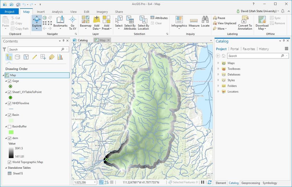
6 Click Run. A dot should appear on your map showing you where the Logan River stream site is. Zoom in on this to get a sense for the topography near Logan. I also changed the symbology of the point to make it easier to see and switched the basemap to Topographic. In the Geoprocessing pane under Portal expand Ready-To-Use Tools to locate and click on the Watershed tool. 6

7 In the Watershed tool set the Input Points to be the feature class created from your spreadsheet (Sheet1_XYTableToPoint). Set Data Source Resolution to FINEST. Leave all other settings at their defaults and click Run. 7

8 When the tool completes you should see the message Watershed completed successfully. You should also see Output Watershed that has been delineated using the online watershed delineation service added to your map. Notice that there is also an Output Snapped Points feature class that contains the outlet point "snapped" or moved to be on the streams. Zoom to layer Output Watershed. Wow, just like that you delineated the stream network of the Logan River. If you like, change the symbology to be more appealing. If you adjust color properties, you can get the watershed to be partly (50%) transparent. Save your project. Now let's get the digital elevation model for this area. We will use the National Map. Obtaining data from the National Map is not always quite as convenient as the ESRI Living Atlas, but it is the authoritative data source, and is available, even if you are not using ArcGIS with an ESRI account, so is a good skill to learn. If downloading the data from the National Map proves excessively time consuming the required data can be obtained from: Go to the National Map Download app 8

9 Zoom in near to Logan in Northern Utah and select Elevation Products (3DEP) then 1/3 arc-second DEM and click Find Products. 9

10 You should see a listing of products similar to The datasets listed are from the selected product within the display area of your map. You can click "Footprint" to see the extent of each dataset. Download the two datasets that cover the Logan River Drainage (using what you have learned about what it looks like from delineating its watershed. 10

11 The two datasets you should download are USGS NED 1/3 arc-second n42w112 and USGS NED 1/3 arcsecond n43w112, The part of the name n43w112 refers to the latitude 43 o N and longitude 112 o W of the North-West Corner of a 1 o x 1 o tile. This DEM is delivered in 1 o x 1 o tiles that will need to be merged. In this case there are just two tiles. For larger watersheds you may need multiple tiles. You should now in your Downloads folder have 2 zip files. Unzip each of these and from each of the unzipped folders add the Raster Datasets grdn42w112_13 and grdn43w112_13 to your map. After zooming out you should see something like 11

12 The two DEM datasets need to be merged. In Geoprocessing find the Mosaic to New Raster tool and set the inputs as follows 12

13 Pixel type needs to be 32 bit float and Number of Bands needs to be 1, consistent with the properties of the DEMs we downloaded from the National Map. You should end up with a single raster demerged that combines the two DEMs downloaded from the national map. Look at the properties of this raster. 13

14 You should see quite a large number of rows and columns, and also that the cell size is x The fact that the coordinate system is Geographic, tells you that this is in decimal degrees. Calculate, for latitude value of 42 o N, following methods learned in earlier homework the cell size in m that corresponds to this decimal degree value x Report the cell size in the N-S and in the E-W direction, as well as the cell area. Assume a spherical earth with radius 6370 km. To turn in: Cell length (N-S) in m, width (E-W) in m, area in m 2 for the DEM cells in the merged DEM. Now let's organize our data into a consistent projection. In the Catalog pane, navigate to your Ex4.gdb geodatabase (automatically created when you create a new ArcGIS Pro project). Note that this already has in it the Sheet1_XYTableToPoint, feature_set, and feature_set1 feature classes from the watershed delineation work at the beginning of the exercise, and the demerged raster. Note that the labels used to display some of these feature classes in the map are different from these feature class names in the geodatabase. In this geodatabase select New/Feature Dataset to create a feature dataset to hold our work. Set the name to Basemap. For the coordinate system select NAD 1983 UTM Zone 12 N. I have chosen to standardize on this coordinate system for this exercise. 14

15 Click Run. Now you have a feature dataset Basemap in your project geodatabase to hold data in the NAD 1983 UTM Zone 12 N Coordinate System. Right click on Sheet1_XYTableToPoint layer in the Map table of and select Data -> Export Features. 15

16 In the Geoprocessing Copy Features tool that opens, set the Output feature class to Gage in the Basemap feature dataset and click Save. Click Run in the Geoprocessing pane to copy these features. This serves to project the geographic coordinates of this site feature class to the UTM Zone 12 N Coordinate System of the Basemap feature dataset. 16

17 Similarly use Data -> Export Features with the Output Watershed layer to copy it into the Basemap feature dataset with name "Basin". This copying to a single feature dataset serves to project the data to a consistent coordinate system (here UTM Zone 12 N) and collect it together in one place in an organized way. It is strictly not necessary for the software, but is a good habit of organization for users. Remove the Output Snapped Points and Outlet Watershed layers. Now let's extract and analyze the DEM for this basin. We use a buffer to select an area slightly larger than the basin to avoid edge effects. Go to the Geoprocessing panel. Search for the Buffer (Analysis Tools) in the geoprocessing toolbox. 17

18 Set the inputs as follows, and run: This produces a feature class BasinBuffer that buffers our basin by 1 km. Next search for the Extract by Mask (Spatial Analyst) tool and set the inputs as follows, saving the output raster in Ex4.gdb\demgc. Note that the DEM is stored at the top level in the geodatabase because a raster cannot be stored in a feature dataset. Note that I used the name demgc to remind myself that this dataset is still in geographic coordinates. The result is a DEM just over the buffered area. 18

19 Next search for the Project Raster (Data Management Tools) tool and set the inputs as follows, saving the output raster in Ex4.gdb\dem. 19

20 Right click on the Map data frame in the table of contents and click on Properties Click on Coordinate Systems and choose NAD 1983 UTM Zone 12N. 20

21 This switches the Map display to the chosen coordinate system. You should see the basin look longer and thinner, which is a better approximation of what it really looks like, compared to the geographic coordinates that were previously in effect. Remove demgc, demerged, grdn43w112_13 and grdn42w112_13. We do not need these anymore. Save your project. To turn in. The number of columns and rows, grid cell size, minimum and maximum elevation values in the Logan River Basin DEM (just named dem above). Hydrologic Terrain Analysis This activity will guide you through the initial hydrologic terrain analysis steps of Fill Pits, calculate Flow Direction, and calculate Flow Accumulation (steps 1 to 3). The resulting flow accumulation raster then allows you to identify the contributing area at each grid cell in the domain, a very useful quantity fundamental to much hydrologic analysis. Next an outlet point will be used to define a watershed as all points upstream of the outlet (step 4). Focusing on this watershed streams will be defined using a flow accumulation threshold within this watershed (step 5). Hydrology functions will be used to define separate links (stream segments) and the catchments that drain to them (steps 6 and 7). Next the streams will be converted into a vector representation (step 8) and more Hydrology toolbox functionality used to evaluate stream order (step 9) and the subwatersheds draining directly to each of the eight stream gauges in the example dataset (step 10). The result is quite a comprehensive set of information about the hydrology of this watershed, all derived from the DEM. 21

22 1. Fill This function fills the sinks in a grid. If cells with higher elevation surround a cell, the water is trapped in that cell and cannot flow. The Fill function modifies the elevation value to eliminate these problems. Select Spatial Analyst Tools Hydrology Fill. Set the input surface raster as dem and output surface raster as fil in Ex4.gdb. Press Run. Upon successful completion of the process, the fil layer is added to the map. Let's examine the impact of Fill on the DEM. Select Spatial Analyst Tools Map Algebra Raster Calculator and evaluate fil - dem. 22

23 Select Spatial Analyst Tools Surface Contour. Set the inputs as follows to determine 20 m contours of the original DEM, dem. Symbolize the fil - dem and contour layers similar to: Zoom in on the deepest Sink; you should see something similar to the image below. 23

24 This is Peter Sink. It is a real topographic feature, not an artifact, so it is a bit erroneous to fill it. Nevertheless for the sake of a complete watershed we fill it. The website gives details on the record low temperatures that have been recorded here. To turn in. A layout showing the deepest sink in the Logan River basin. Report the depth of the deepest sink as determined by fil-dem. 24

25 2. Flow Direction This function computes the flow direction for a given grid. The values in the cells of the flow direction grid indicate the direction of the steepest descent from that cell. Select Spatial Analyst Tools Hydrology Flow Direction. Set the inputs as follows, with output "fdr" and "drp". Press Run. Upon successful completion of the process, the flow direction grid "fdr" and percentage drop grid "drp" are added to the map. 25

26 To turn in: Make a screen capture of the attribute table of fdr and give an interpretation for the values in the Value field using a sketch. 3. Flow Accumulation This function computes the flow accumulation grid that contains the accumulated number of cells upstream of a cell, for each cell in the input grid. Select Spatial Analyst Tools Hydrology Flow Accumulation. Set the inputs as follows. Note that I selected an Integer output type because we are not using a weight raster input and the result is a count (integer) of the number of upstream grid cells that drain into each grid cell. Press Run. Upon successful completion of the process, the flow accumulation grid fac is added to the map. This process may take several minutes for a large grid, so take a break while it runs! Adjust the symbology of the Flow Accumulation layer "fac" to a classified scale with multiplicatively increasing breaks that you type in, to illustrate the increase of flow accumulation as one descends into the grid flow network. Use the Classify Button to enable you to select Manual Interval method and to type in your class breaks into the Upper value window in the Class breaks section. 26

27 After applying this layer symbology you may right click on the "fac" layer and Sharing -> Save As Layer File 27

28 The saved Layer File may be imported to retrieve the symbology definition and apply it to other data. Pan and zoom to the outlet where the river leaves the watershed. Turn off unnecessary layers and arrange layer order so that you can see the Basin feature class on top of the fac layer. Use the identify tool to determine the value of "fac" at the point where the main stream exits the area defined by the Basin polygon. This location is indicated in the following figure. The value obtained represents the drainage area in number of 10 x 10 m grid cells. Calculate the drainage area in km 2. Compare this drainage area to the drainage area reported by the USGS at the Logan River stream site (214 mi 2 ) and to the area of the Basin feature class obtained from the online service watershed delineation. 28

29 To turn in: Report the drainage area of the Logan River basin in both number of 10 m grid cells and km 2 as estimated by flow accumulation. Report the area of the Logan River basin in km 2 as calculated by the arcgis.com watershed function. Report the area of the Logan River basin in km 2 as reported by the USGS for the Logan River stream site. Discuss reasons for any differences. 4. Stream Definition Let's define streams based on a flow accumulation threshold within this watershed. Select Spatial Analyst Tools Map Algebra Raster Calculator and enter the following expression, using the name Str for the output raster. 29

30 The result is a raster representing the streams delineated over our watershed. This extends across the buffer area at the downstream end. To ensure that our streams are within the watershed we want let's clip this. Locate the Extract by Mask (Spatial Analyst) tool and set the inputs as follows: The result is a stream raster entirely within the Logan River Basin. 30

31 5. Stream Links This function creates a grid of stream links (or segments) that have a unique identification. Either a link may be a head link, or it may be defined as a link between two junctions. All the cells in a particular link have the same grid code that is specific to that link. Select Spatial Analyst Tools Hydrology Stream Link. Set the inputs as follows and click OK. The result is a grid with unique values for each stream segment or link. Symbolize strlink with unique values so you can see how each link has a separate value. 31

32 6. Catchments The Watershed function provides the capability to delineate catchments upstream of discrete links in the stream network. Select Spatial Analyst Tools Hydrology Watershed. Set the inputs as follows. Notice that the Input raster or feature pour point data is the strlink grid. This results in the identification of catchments draining to each stream link. Click OK. The result is a catchment grid where the grid cells in the area draining directly to each link are assigned a unique value the same as the link it drains to. This allows a relational association between lines in the strlink grid and area's in the catchment grid. Symbolize the catchment grid with unique values so you can see how each catchment has a separate value. 32

33 7. Conversion to Vector Let's convert this raster representation of streams derived from the DEM to a vector representation. Select Spatial Analyst Tools Hydrology Stream to Feature. Set the inputs as follows. Note that I named the output drainageline in the Ex4_project.gdb\BaseMap feature class. Note here that we uncheck the Simplify polylines option. The simplification can cause streams to "cut corners" that can result in errors. The result is a linear feature class "drainageline" that has a unique identifier associated with each link. Select Conversion Tools From Raster Raster to Polygon. Set the inputs as follows again avoiding simplification of polygons, but also setting to Create multipart polygons 33

34 The result is a Polygon Feature Class of the catchments draining to each link. Due to the geometry of grid cells in catchment, you may get multiple polygons for a single catchment grid code value. However by selecting the multipart option above they are combined into one multipart polygon. The feature classes drainageline and catchpoly represent the connectivity of flow in this watershed in vector form. To turn in: The number of drainageline segments and catchments delineated from this DEM. To turn in: Describe (with simple illustrations) the relationship between strlink, drainageline, catchment and catchpoly attribute and grid values. What is the unique identifier in each that allows them to be relationally associated? To turn in. Prepare a layout showing the stream network and catchments delineated directly from the DEM. To turn in. Report the total stream length, basin area and drainage density for the Logan River Basin as determined from the DEM delineated streams. Based on drainage density calculate the average overland flow distance water originating on a hillslope has to travel before reaching a stream. [Hint: Refer to slide 35 from ExtendedTerrainAnalysis.pptx in lecture 10.] 34

35 Zoom in to the North edge of the basin and you can see that there is a difference between the watershed boundary as delineated from the online watershed delineation tool and 10 m DEM. Prepare a layout that illustrates this discrepancy and estimate the difference in Logan River drainage area due to this discrepancy. (Note that "estimate" is key here. It is OK to measure differences and estimate area approximately. We are not looking for an elaborate GIS analysis to determine this discrepancy precisely. To turn in: Layout illustrating discrepancy in watershed boundary at the North end of Logan River basin. Report your estimate of the Logan Watershed area difference in km 2 due to this discrepancy. Comparison with National Hydrography Dataset (NHDPlus V2.1) 1. Obtaining NHDPlus Data NHD Plus data is available from Click on Version 2, Data and Great Basin 16 in the map to get to Download NHDPlusV21_GB_16_NHDSnapshotFGDB_06.7z and NHDPlusV21_GB_16_EROMExtension_03.7z In case there are problems with data downloaded from this source, the required information can be obtained from: 35

36 You can read more about this dataset in the documentation if you are interested ftp://ftp.horizonsystems.com/nhdplus/nhdplusv21/documentation/nhdplusv2_user_guide.pdf. You should have two files in your downloads. Put these in your Ex4 folder and use a zip program to Extract Here. Both should unzip into the same NHDPlusGB folder. GB stands for Great Basin. Add NHDFlowline.shp to your map. 36

37 You should get 37

38 Add the table (dbf file) EROM_MA0001.dbf to your map Open the table EROM_MA0001 From reading the documentation column Q0001E holds flow from gage adjustments in cfs. Let's join this to NHDFlowline. If the version of NHDFlowline you have does not contain a COMID field, the required information is contained in the field Permanent_Identifier. However, this is a text field and to make the join work, the field types for both tables need to be the same, namely Long integer. To fix this, Add a field to the NHDFlowline table for COMID, with type Long, and then Calculate the value of this field as COMID = Permanent_Identifer. You can then proceed with the exercise. Alternatively, an 38

39 NHDPlus flowline dataset with the COMID field already available is accessible at: Right click on NHDFlowline and select Joins and Relates -> Add Join. 39

40 In the Add Join Tool set inputs as follows, noting that ComID is the common identifier field used to join tables in NHDPlus. Click Run. If you examine the NHDFlowline attribute table now you will see that EROM_MA0001 attributes have been joined. Use Select Layer By Location to select features from NHDFlowline that Have their center in Basin, the watershed that was delineated online earlier. 40

41 You should see just the streams within the basin selected 41

42 Right click on NHDFlowline and select Data -> Export Features to open the Copy Features tool and set the Output Feature Class as NHDStreams in the BaseMap Feature Dataset. Click Run. Note that by saving the result in this feature dataset the copy process also projects the data (just the selected data) to the coordinate system of the feature dataset. Also, since flow attributes were joined these are retained in the NHDStreams feature class written to the Basemap feature dataset. Remove NHDFlowline from the map and Save. 42

43 You should now see just the extracted NHDStreams features on your map view. Symbolize NHDStreams using gage adjusted flow E (Q0001E) to give a flow map. In the Symbology panel, select Graduated Symbols and Q0001E for the field. Click on Template and set the color, and apply. To turn in: Prepare a layout showing NHDPlus streams within the Logan River Basin symbolized using line width scaled by gage adjusted flow. Report the mean annual gage adjusted flow at the most downstream segment in the Logan River drainage from NHD plus. Compare this mean annual flow to the mean annual flow from the Logan River stream gage. 2. Main Stream Properties In this section we do the following - Use ArcGIS pro query functionality to select the Logan River main stream - Use Summary Statistics tool to tabulate stream length - Use stream length and area data to calculate drainage density and average hillslope length To identify the main stem of the Logan River and determine some of its properties open the Select By Attributes geoprocessing tool in the Map tab. 43

44 Click and configure a query to select where GNIS_NAME is Equal to Logan River. Click Click Run in the geoprocessing tool. The Logan River main stream should be selected. 44

45 Right click NHDStreams layer and select Data Export Features and save the selected features as LoganMain in the Logan.gdb\Basemap feature dataset. This is a feature representing just the Logan River. Once the LoganMain Feature Class has been written you should clear selection to remove selection from the map view. Let's examine the length of LoganMain. Open the attribute table of LoganMain. Note that there are multiple columns that give length. LENGTHKM is length in km from the NHD. shape_length is the far right column and is the length evaluated by ArcGIS when the data was loaded into the geodatabase. All geodatabase features have geometry measures (e.g. length or area). The units of shape_length are the 45

46 units of the feature dataset coordinate system, which are meters in this case. You should note consistency between LENGTHKM and shape_length once units are converted. Right click on the column header Shape_Length of the far right column and select Summarize. Add the fields LENGTHKM and shape_length and the statistic type SUM. Note the name of the output table. Make sure that the Case field is blank and run. Open the resultant statistics table that was output: 46

47 Note the values of Sum. These are the length of LoganMain (the Logan River main stream) from the two length fields. Note that they should be numerically close once the shape_length is converted to km. They differ due to different approximations and coordinate systems being used here, and by NHDPlus. Similarly, create a statistical summary of the NHDStreams feature class to determine the total length of streams in the Logan River Basin. Lastly, open the attribute table for Basin and look for the far right column Shape_Area. This is the Basin area in m 2. Calculate the drainage density for the Logan River as (Total Channel Length)/(Basin Area). At this point you have extracted all the data you need locally and are ready to begin Hydrologic Terrain Analysis. To turn in. Prepare a layout showing the topography, Basin Outline, NHDPlusV2 streams, and Logan River Main stem stream for the Logan River Basin. Include a scale bar and North arrow and appropriate title, labeling and legend so that the map is self-describing. To turn in. Report the main stream length, total stream length, basin area and drainage density for the Logan River Basin as determined from NHDPlus flowlines. Comment on the differences between this drainage density and the DEM derived drainage density. OK. You are done! Summary of items to turn in. 1. Cell length (N-S) in m, width (E-W) in m, area in m 2 for the DEM cells in the merged DEM. 2. The number of columns and rows, grid cell size, minimum and maximum elevation values in the Logan River Basin DEM 3. A layout showing the deepest sink in the Logan River basin. Report the depth of the deepest sink as determined by fil-dem. 4. Make a screen capture of the attribute table of fdr and give an interpretation for the values in the Value field using a sketch. 5. Report the drainage area of the Logan River basin in both number of 10 m grid cells and km 2 as estimated by flow accumulation. Report the area of the Logan River basin in km 2 as calculated by the arcgis.com watershed function. Report the area of the Logan River basin in km 2 as reported by the USGS for the Logan River stream site. Discuss reasons for any differences. 6. Describe (with simple illustrations) the relationship between StrLnk, DrainageLine, Catchment and CatchPoly attribute and grid values. What is the unique identifier in each that allows them to be relationally associated? 7. Prepare a layout showing the stream network and catchments delineated directly from the DEM. 8. Report the total stream length, basin area and drainage density for the Logan River Basin as determined from the DEM delineated streams. Based on drainage density calculate the average overland flow distance water originating on a hillslope has to travel before reaching a stream. [Hint: Refer to slide 35 from ExtendedTerrainAnalysis.pptx in lecture 10.] 47

48 9. Layout illustrating discrepancy in watershed boundary at the North end of Logan River basin. Report your estimate of the Logan Watershed area difference in km 2 due to this discrepancy. 10. Prepare a layout showing NHDPlus streams within the Logan River Basin symbolized using line width scaled by gage adjusted flow. Report the mean annual gage adjusted flow at the most downstream segment in the Logan River drainage from NHD plus. Compare this mean annual flow to the mean annual flow from the Logan River stream gage. 11. Prepare a layout showing the topography, Basin Outline, NHDPlusV2 streams, and Logan River Main stem stream for the Logan River Basin. Include a scale bar and North arrow and appropriate title, labeling and legend so that the map is self-describing. 12. Report the main stream length, total stream length, basin area and drainage density for the Logan River Basin as determined from NHDPlus flowlines. Comment on the differences between this drainage density and the DEM derived drainage density. 48