Exercise 5 - Watershed and Stream Network Delineation from DEMs GIS in Water Resources Fall 2014

Transcription

1 1 Exercise 5 - Watershed and Stream Network Delineation from DEMs GIS in Water Resources Fall 2014 Prepared by Ayse Kilic and Bhavneet Soni 1 University of Nebraska-Lincoln This exercise illustrates watershed and stream network delineation using digital elevation models (DEM) using the Hydrology tools in ArcGIS and online services for Hydrology and Hydrologic data. In this exercise, you will develop a stream basin by selecting a stream gage location (the USGS discharge gauge (USGS station ID ) on the Loup River near Genoa, Nebraska) and using the ArcGIS online tools to delineate the watershed draining to the gage. National Hydrography (NHD flowline) and Digital Elevation Model (NED30m) data will be retrieved for the Loup River Basin from online services. You will then perform drainage analysis on a terrain model for this area. The ArcGIS Hydrology tools will be used to derive several terrain parameter data sets that describe the drainage patterns of the basin. Geoprocessing analysis is performed to fill sinks (pits) and to generate data on flow direction, flow accumulation, catchments, streams, stream segments, and watersheds. These data are then used to develop a vector representation of catchments and drainage lines from selected points that can then be used in network analysis. This exercise shows how connectivity between the landscape and streams can be developed starting from raw digital elevation data, and that this enriched information can be used to compute watershed attributes commonly used in hydrologic and water resources analyses. Background on the Loup River From Wikipedia: The Loup River is a tributary of the Platte River, approximately 68 miles (109 km) long, in central Nebraska. The river drains a sparsely populated rural agricultural area on the eastern edge of the Great Plains southeast of the Sandhills. The name of the river means "wolf" in French, named by early French trappers after the Skidi band of the Pawnee, whose name means "Wolf People," and who lived along its banks. The river and its tributaries, including the North Loup, Middle Loup, and South Loup, are known colloquially as "the Loups", comprising over 1800 mi (2900 km) of streams and draining approximately one-fifth of Nebraska. A diversion dam southwest of Genoa diverts water to the Loup Canal to hydroelectric facilities in Monroe and then in Columbus. The canal then runs into the Platte a short distance below its confluence with the Loup. 1 Some of the materials and structure for this exercise originated from Dr. David Tarboton, Utah State University.

2 2 Learning Objectives The objectives of this exercise are to delineate the watershed and stream network for a selected basin using DEM and spatial analyst tools in ArcGIS. We will also delineate the watershed using online delineating tools. The processing will include: 1. Downloading and Importing Gauge station location (Point Data) 2. Downloading the DEM and NHD data from ESRI Online Sources 3. Extracting the DEM data 4. Delineating the Watershed from DEMs 5. Network Delineation 6. Network Analysis Special requirements for the Exercise We need to activate the Spatial Analyst extension before we proceed with the exercise. Once you have activated it on your computer you do not need to repeat this step again Select Customize Extensions Select 3D Analyst and Spatial Analyst extension. We will be using these during the exercise.

3 3 You also need to be subscribed to the ArcGIS online services. This is done by obtaining an invitation from the administrator of the UNL account. This invitation will be arranged by the instructor. You will need to activate the invitation. Part 1: Online Watershed Delineation and Data Retrieval from ESRI A watershed is the total drainage area upstream of a point. For this exercise we will delineate the watershed upstream of the USGS Stream Gauge site on the Loup River near Genoa, Nebraska. 1.1 Adding the USGS Gauge station to the Map We need to add the Gauge Station s coordinates to ArcMap. Information about the gauge station can be found at the USGS water data website, map viewer: Zoom in to the area and locate the gauge station. Otherwise, you can search for the station ID number

4 4 Click on the Access Data to get location information. Transfer the geographical information into an excel spreadsheet and convert the latitude/ longitude from degrees, minutes, seconds to decimal degrees. (Decimal Degrees = degree + minutes/60 + seconds/3600). Following the steps from previous exercises, add the spread sheet to ArcMAP and display XY data based on the LAT DD (for Y) and Long DD (for X) columns. You will want to make sure you select NAD83 as the coordinate system (see below). Right click on this spreadsheet layer and select Display XY data.

5 5 Set the X and Y fields. Recall that the USGS NWIS website indicated a NAD83 coordinate system. Click Edit to edit the coordinate system Locate Geographic Coordinate Systems North America NAD1983 in the Spatial Reference Properties window and click OK.

6 6 Now you have the Gauge station in NAD83 coordinate system in the map. Let s now add a topographic base map to serve as a background in the viewer, so that we have some frame of reference where our gauge is.

7 7 You can see our gauge station is on the Loup River near Genoa. We should export the data as a feature dataset or a shape file. However, before we do that, let s open Arc Catalog and create a folder and a geodatabase to store your files. You are going to be creating a lot of files from terrain preprocessing. It is important that you create a Geodatabase to store and organize output files. In addition, some of the terrain processing tools will give you error or will not run without the output location set into a Geodatabase. Now let's set up a folder and geodatabase for your work. First create a folder (for instance, for the instructor: C:\Ayse\Ex5\Sol1). Then, save the map document in this folder (Ex5.mxd). This serves to

8 8 establish a place on disk where temporary files can be written and a Home location in Catalog. Now, create a new Geodatabase and name it Loup.gdb. Inside the Loup.gdb, create a feature data set and name it Basedata and set its Projection coordinates as Albers Equal Area Conic. The Albers Equal Area Conic is usually the best projection system for preserving area. Click Next, Next and Finish. Now let s export the data, Right click on the Events layer Save the file as Gauge in the BaseData Feature dataset under your Loup GDB. Placing the Gauge feature inside the BaseData feature will automatically adopt the Albers projection of the BaseData feature. This serves to project the geographic coordinates of this site feature class to the North America Albers coordinate system of the BaseData feature dataset and make it a permanent feature class. Remove Sheet1$ Events.

9 9. Online watershed Delineation and Data Retrieval 1.2. Elevation Data To do any kind of watershed or water flow analysis you need to have Elevation information. The next step is to add Elevation data to the map.

10 Open ArcCatalog. Double Click on Add ArcGIS Server. Select Use GIS Services, the first option. 10

11 11 Enter the Server URL and your ArcGIS.com user name and password. Note that username and password are case-sensitive. You should see ARCGIS on elevation.arcgis.com displayed in your Catalog under GIS Servers.

12 12 Expand the tool to see the services available NED30m is the USGS National Elevation Dataset digital elevation model. Drag and drop NED30m from ArcCatalog onto your ArcMap to add this data to the ArcMap data frame. Close the coordinate systems warning. You may have to try this a few times before the NED30m shows up in ArcMap. Make sure you have both windows for Arc Catalog and ArcMap is open.

13 13 The first view in ArcMap look like the following. You can then zoom in to the gage for the Loup River Watershed tool in the Hydrology toolbox Now we are going to add the Watershed tool in the Hydrology toolbox. The server url is at

14 14

15 Now locate the watershed tool in the Hydrology toolbox in Arc Catalog. We are going to create a watershed representing all contributing areas above Loop River gage at Genoa. 15

16 16 Click on watershed and set Input Points to Gauge (the Loop River stream site). Set Data Source Resolution to 30 meter. Leave other inputs at their defaults and click OK to run the tool. When the tool completes, you should have an Output Watershed that has been delineated using the ESRI online watershed delineation service. It appears in the GPInMemoryWorkspace part of the map document table of contents. You need to have List by Source option selected for Table of Contents (TOC). Notice that there are two layers listed: Output Watershed which shows the outline of our watershed boundary of the Loup River above Genoa. The second feature is called Output Snapped Points and contains the outlet point "snapped" or moved to be on the stream. We will use this later on the exercise.

17 17 Right click on Output Watershed and select Data and Export Data to export this delineated watershed and name the output feature class as Basin in Loup.gdb\BaseData. This saves the Basin feature class on your computer. We will be using this Basin basemap to extract data. This is our study domain.

18 18 Likewise, save the Output Snapped Points in Loup.gdb\BaseData\GageSnap feature class. Saving these results locally retains them in case you have to restart. If that happens, the GPInMemoryWorkspace would be lost and you would have to repeat this procedure.

19 19 Let s zoom in near the outlet of the Loup River basin (Genoa guage). Note whether or not the location of the gauge has been shifted relative to the original location that you used. This is to move the outlet onto the stream flow path in the preprocessed NED30m DEM that underlies the watershed delineation. Estimate the amount of shift and why it occurred. Which location do you conclude is the most accurate and why.

20 20 Notice that our watershed boundary has a stair step shape (the green color above) because it is based on DEM grid cells. Check to make sure that the underlying NED30m DEM coordinate system is the same as the display data frame. If not, you would need to change data frame to the coordinate system of the DEM. Check this by Right clicking and evaluating the projection system. Compare that information with the same thing for the DEM. Extracting the DEM for the Basin from NED30m Next we want to extract the DEM for this area. Here we want the DEM over an area slightly bigger than the watershed. Let's use a 1 km buffer.

21 21 Search for the Buffer (Analysis) tool and set the inputs as follows This process may take several minutes to complete (watch the lower righthand part of your screen for progress). When finished, the basin will now be outlined by the buffered basin feature that is 1 km larger (see following figure where the basin and buffered basin are viewed with no fill):

22 22 Next, we will search for the Extract by Mask (Spatial Analyst) tool and set the inputs as follows The result is a DEM over the buffered area of the basin. This DEM is 1 km larger than the Loup River basin so that we have no problems during calculations of terrain parameters including slope and flow direction.

23 23 This completes the downloading and extraction of the DEM from the online services. The DEM is now ready for terrain analysis. To turn in: The number of columns and rows, and grid cell size in the Loup River basin DEM. The minimum and maximum elevation values in the Loup River basin DEM. The next step is to bring in the NHD flow line data National Hydrography Data Service (NHDPlusV2). Next we are going to bring in flowlines that have been preprocessed by ESRI and are made available via ArcGIS server. This product is only available via the online subscription. When possible, it is best to use the online data to save processing, downloading, unzipping time. In Catalog, under GIS Servers add the ArcGIS service as you did before for elevation and hydrology services.

24 24 Under Tools in the Landscape 1 service, double click on Extract Landscape Source Data (see image below) and choose NHDPlus V2 Flowlines as the Landscape Layer and Basin as the study area. Wait until this message box appears Open the Geoprocessing Results Window in ArcMAP (in the top menu):

25 25 Expand the current session and you will see a NHDPlusv.zip file appear. Double Click to open the output zip file and copy the geodatabase folder Landscape.gdb that is inside the zip file into the folder where you are working (for example: C:\Ayse\Ex5\Sol1). (Click on the

26 26 Landscape.gdb to select it, right click and select copy and then go to your working folder (for example C:\Ayse\Ex5\Sol1). Do the copy and paste in the same Explorer window): Add the feature class NHDPlusv from Landscape.gdb (that is in your working folder) to the ArcMap display and symbolize using Gage Adjusted Flow E to give a flow map. Under Symbology, select Quantities and Graduated colors. Ignore warnings. Format the labels.

27 27 This is now a local set of NHDPlus vector streamlines for the Loup River Basin Main Stream Properties Let's now identify the main stem of the Loup River, including the Middle Loup River, and determine some of its properties. Open the attribute table for NHDPlusv. Select By Attributes and click on Get Unique Values to see the names of the stream. Note: The hydrographic GNIS names contained in and displayed by the NHD are from the GNIS (Geographic Name Information System) database which holds the Federally recognized name of each feature and defines the location of the feature by state, county, USGS topographic map, and geographic coordinates. You need to write a Query to select where gnis_name = 'Loup River' OR gnis_name = 'Middle Loup River'

28 The query will select both main stem and middle loop rivers and they should display as a highlighted color. 28

29 29 Now we will export the selected Loup and Middle Loup entries. Right click on the NHDPlusv layer and select Data Export Data and save the selected features as LoupMain in the Loup.gdb\Basedata feature dataset. This is a feature that contains only information on the Loup and Middle Loup rivers (but none of their tributaries). Let's examine the length of the mainstem Loup (and Middle Loup) River from its source to this outlet (Genoa gauge). In the attribute table of LoupMain locate the column "Length (km)" and Right click on the header and select Statistics

30 30 Note the Sum value and the units (the length of the Loup and Middle Loup River from its source to this outlet at Genoa gauge). To turn in. Prepare a layout showing the topography (DEM), Basin Outline, NHDPlusv streams and Loup River Main stem and Middle Loup streams for the Loup River Basin. Include a scale bar and North arrow and appropriate title, labeling and legend so that the map is self-describing. Part 2. Hydrologic Terrain Analysis This activity will guide you through the initial hydrologic terrain analysis steps of Filling Pits, calculating Flow Direction, and calculating Flow Accumulation (steps 1 to 3). The resulting flow accumulation raster will allow you to identify the contributing area at each grid cell in the domain, a very useful quantity fundamental to hydrologic analysis. Next an outlet point will be used to define a watershed as all points upstream of the outlet (step 4). Focusing on this watershed, streams will be defined using a flow accumulation threshold within the watershed (step 5). Hydrology functions will be used to define separate links (stream segments) and the catchments that drain to them (steps 6 and 7).

31 31 Next the streams will be converted into a vector representation (step 8) and more Hydrology toolbox functionality used to evaluate stream order (step 9) and the subwatersheds draining directly to each of the eight stream gauges in the example dataset (step 10). The result is a comprehensive set of information about the hydrology of this watershed, all derived from the DEM. Step 1: DEM Conditioning (Fill Pits) Search and Run the Fill tool to fill in the Sinks in the DEM. Sinks are the cells that are surrounded by cells all having an elevation higher than it, i.e the water will not flow anywhere from the pit cell. Running this tool is very memory and CPU intensive and will take a long time. Save the file into the Geodatabase. Select Spatial Analyst Tools Hydrology --> Fill. Set the input surface raster as DEM and output surface raster as fill in Loup.gdb. Let's examine the impact of Fill on the DEM. Select Spatial Analyst Tools Map Algebra Raster Calculator and evaluate the differences between FILL and the original DEM by calculating the difference FILL DEM in Raster Calculator. Save the result as FillMinusDEM.

32 32 View this difference map. Comment on the differences, where they occur, and why they occur. You should on an area to make this assessment. If you see lots of pits, especially in the Sandhills area, suggest what these pits are, in reality. To help with your assessment, also create a Contour map from the DEM. Select Spatial Analyst Tools Surface Contour. You can set the Contour interval to 10 m. An overlay of the Contour lines on top of the FillMinusDEM map, where the map is colorized to show low values as green and large values as blue is shown below:

33 33 The above figure on the left is a closeup of the boxed area in the west central part of the Loup River Basin. That figure, with contours and colorized differences (showing filled pits), may give you a better idea of what these features are. (The circled area is commented on later). Question: what are these, and should they be filled?

34 34 Step 2. Flow Direction To delineate the Watershed, we should know which way the water is flowing from a cell. To determine this, search for tool Flow Direction. This tool compares each cell with its neighboring cells to determine the direction of steepest descent, and therefore, where each cell is draining to. Flow Direction Tool applied to the Fill DEM. Flow direction is saved as FDR and the Drop raster is saved as DRP. If we zoom in to the same area as above (for the FillMinusDEM), we can see the actual detail for specific slopes:

35 35 Note that some of these shapes have straight edges. This occurs because the flowline (direction) has been determined for the pit-filled areas, and these areas are perfectly flat after the filling. Therefore, the direction tool gets confused and assigns a variety of directions. The following snapshot is along the Middle Loup River and shows the drainage of south-facing slopes and north-facing slopes into the river:

36 36 Step 3.Flow Accumulation Once we know the Flow direction we can ascertain how the flow is getting accumulated and where small groups of cells turn into streams and where streams turn into rivers. Search for the Flow Accumulation tool or Spatial Analyst Tools Hydrology Flow Accumulation. Use the Flow direction as the input raster and save the output in to the Geodatabase as FAC. The Flow Accumulation tool is a very CPU and Memory intensive process. You will need to be patient. Have some coffee. Watch an old episode of Friends and relax. This tool will take substantially more time than it took to make the Flow Direction raster (it may take about 1 hour). The initial result in the viewer will look like the following:

37 37 The result initially looks like just a black screen because all values close to zero are colored black, but there are some cells in the main river having high values for accumulated cells. Therefore, the color stretch shows most cells as black. If you zoom in you will see some of the stream structure. Adjust the symbology of the Flow Accumulation layer to a classified scale with multiplicatively increasing breaks that you type in, to illustrate the increase of flow accumulation as one descends through the grid flow network. In symbology, use 8 classes and select the Classify Button and choose the Manual method to type in your class breaks in the window in the lower right hand corner of the menu window.

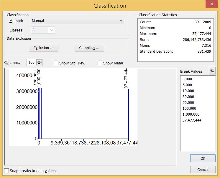
38 38

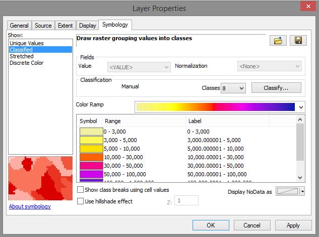
39 39

40 40 Turn off the unnecessary layers and pan and zoom to the outlet of the outlet of the basin, which is at the Genoa Gaging Station. This location is indicated in the following figure. Use the identify tool to determine the value of "FAC" at the outlet. The value obtained represents the drainage area in number of 30 x 30 m grid cells. Calculate the drainage area in km 2. Turn in the drainage area into the gauge station in both number of 30 m grid cells and as km 2 as estimated by the flow accumulation tool. Compare this to the area of the basin, as a check where the area of the basin is obtained from two different sources: a) from the attribute table for the basin, and b) from the USGS properties menu for the Genoa gage as shown below. Also, determine why the Drainage area in the USGS Description has a dfferent value than the contibuting drainage area for this particular basin(think about what we have dicussed under the flow direction analysis).

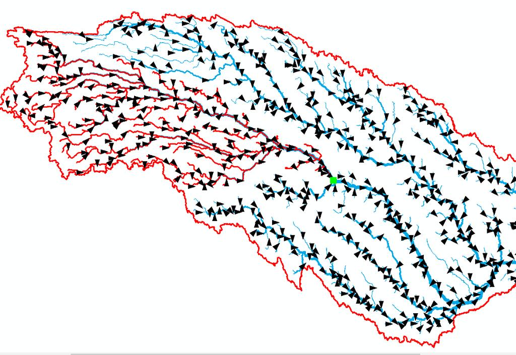
41 41 Step 4: Watershed We will run the Watershed tool twice. The first time we run it, we will ask for delineation of all of the watershed above the Genoa gauge. This will give us a single watershed unit. The second time through, we will run the Watershed tool using stream segments (links) to delineate small catchments throughout the basin. Note that we already have the entire watershed via the watershed tool from the ESRI online watershed delineation service that was run earlier. But it is a good check to do it again, plus to see the outcome. Before we can use a single point as the pour point in the Watershed tool, we need to snap the gauge location to the 30 m cell that has the highest FAC, and we turn that location into a 30 m equivalent size. We do this using the Snap Pour Point tool: The result of the Snap Pour Point will be a single raster layer that has the value of the maximum FAC and it will be the size of one 30 m cell (the red cell in the following screenshot, where the blue symbol is the original location of the gauge and the green cell is the location when previously snapped to the ESRI online watershed tool) :

42 42 For the first time through: Search and run the Watershed Tool using the Snap_to_FAC as the feature pour point data and FDR as input: Use the Flow direction raster (FDR) for Input flow direction and the Snap_to_FAC for feature point data. It is important to use the 30 m Snap_to_FAC raster point to make sure that the Watershed tool sees

43 43 that the outlet cell is located on the maximum accumulation cell. The result should be a Watershed raster that has the value 1 over the area upstream from the outlet point. The following is a result (in green) when using the filled DEM-based flow direction and flow accumulation tools. The purple line is the basin boundary derived from the online Watershed tool. Notice that there is some disagreement at a few locations along the edge. Step 5. Delineating the Stream Network Stream networks can be delineated from a Digital Elevation Model (DEM) using the output from the FLOWDIRECTION and FLOW ACCUMULATION tools. Flow accumulation, in its simplest form, is the number of upslope cells that flow into a particular cell. By applying a threshold value to the values of FLOWACCUMULATION, a stream network can be defined that is comprised of catchments that are of the size of the threshold value. For this exercise we will explore the effect of using a thresholds of 5,000 (a standard value) and 30,000 cells. Search and open the Raster Calculator and apply the query of FAC > 5000 and Watershed_FAC > 0. The Watershed_FAC > 0 will cause the accumulation to apply only to our watershed. Save the result as STR5000. Run the Calculator a second time and apply the query of FAC > Save the result as STR ("FAC" > 5000) & ("Watershed_FAC" > 0)

44 The result is a raster representing the streams delineated over our watershed that have flow accumulation > 5000 and that are inside the watershed boundary. 44

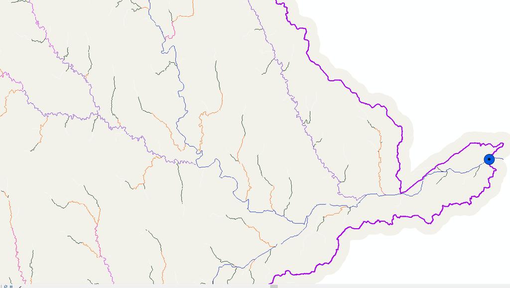
45 45 The raster image shows the Streams (Blue color) where the flow accumulation is more than 5,000 grid cells within the watershed. Now let s change the color of 0 Values (Cells with Flow Accumulation < 5,000) to no color, you can zoom and see the layout of various streams. For the 30,000 threshold (results below), the streams are much shorter and less dense. This makes sense, since 30,000 cells must accumulate before we call something a stream.

46 46 Step 6. Stream Links The Stream Link function creates a grid of stream links (or segments) that have a unique identification. A link may be a head link, or it may be defined as a link between two junctions. All cells in a particular link have the same grid code that is specific to that link. Search and run Stream Link Tool

47 47 The result is a grid with unique values for each stream segment or link. Symbolize StrLnk5000 with unique values so you can see how each link has a separate value. The streams look like the results from the raster calculator above. Run the same Stream Link tool for the 30,000 cell threshold and call the results StrLnk Catchments The Watershed function provides the capability to delineate unique catchments upstream of discrete links in the stream network. Run the Watershed tool again but this time use the input raster as the strlnk. Run this tool twice, once using StrLnk5000 and once using StrLnk30000.

48 48 The result is a Catchment grid where the subcatchment area draining directly to each link is assigned a unique value that is the same as the link it drains to. This allows a relational association between lines in the StrLnk grid and Area's in the Catchments grid. Symbolize the Catchments grid with unique values so you can see how each catchment has a separate value. Catchments when threshold is set to 5000.

49 49 Catchments when threshold is set to Closeup view of catchments and streams when threshold is set to 5000.

50 50 Closeup view of catchments and streams when threshold is set to Questions: Compare the two catchment grids (based on 5000 and 30,000 thresholds). Which one appears to present the best representation of catchments for purposes of hydrologic modeling? Justify your answer. Based on the close ups, what are the primary differences between the two catchment maps? Step 7. Conversion to Vector Let's convert the raster representation of streams derived from the DEM to a vector representation. This is useful to reduce disk storage requirements and to create a continuous vector or each stream segment that can identified in a hydrologic model and that is independent of the raster grid. Search and Run Stream to Feature tool for the threshold data. Remember that the vector result is a feature and should be saved under the feature class Basedata that we created earlier. Also make sure to uncheck the Simplify Polylines checkbox.

51 51 The simplify polygons option can cause streams to "cut corners" that will result in errors when they are later matched with values on an underlying stream order grid during the process of determining stream order. The result is a linear feature class "DrainageLines_30000" that has a unique identifier associated with each link. Similarly convert the Watershed and Catchments into polygons by using Raster to Polygon tool

52 52

53 53 The results are a Polygon Feature Class of the catchments draining to each link. The feature classes DrainageLine and CatchPoly represent the connectivity of flow in this watershed in vector form and will be used later for some Network Analyses, that requires having these data in vector form. The following screenshot shows the polygons for the threshold catchments, with the red boundary the polygon created from the Watershed_FAC feature. If we turn on the drainagelines_30000 polygons that represent the stream network, we get the following:

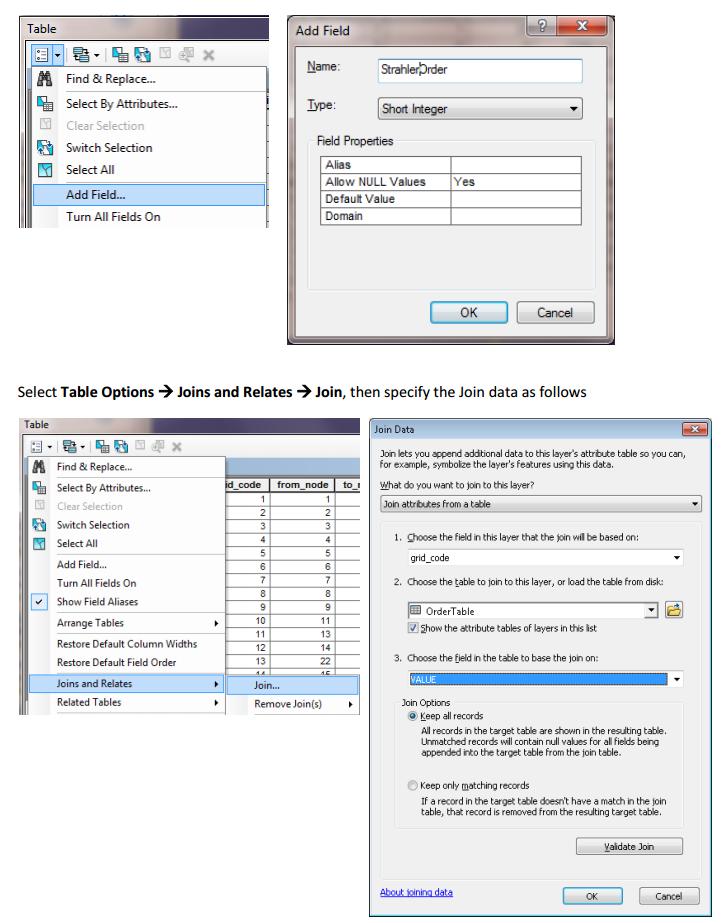
54 54 Turn in Screenshots of the last two figures showing the polygons of catchments and then also with overlays of the stream segment lines. Describe (with simple illustrations) the relationship between StrLnk, DrainageLine, Catchments and CatchPoly attribute and grid values. What is the unique identifier in each that allows them to be relationally associated? Step 8: Strahler Stream Order Stream order is used to define stream size based on a hierarchy of tributaries,

55 55 Search and run tool Stream Order The result is a Raster StrahlerOrder that holds Strahler Order values for each grid cell. Let's now associate these with the streams represented by DrainageLine. Locate the Zonal Statistics as Table (Spatial Analyst) tool and run it with inputs as follows

56 56 The result is a Table "OrderTable" that has zonal statistics from the StrahlerOrder grid corresponding to each link in the StrLnk grid. Open the DrainageLine attribute table. Select Table Options Add Field. Specify the name StrahlerOrder and leave other properties at their default. (Strahler Orders are small integer numbers that should fit in a Short Integer data type)

57 57

58 58 The DrainageLine table now displays many more columns because it has included all the columns from OrderTable. Since the Strahler Order is the same for each link, the fields MIN, MAX, MEAN, MAJORITY, MINORITY, MEDIAN all hold the same value, the stream order and any one of these can be copied into the StrahlerOrder field we just created. Right Click on the StrahlerOrder field header and select Field Calculator. Click Yes to the warning about working outside an edit session, then double click on the OrderTable. MIN field so that the Field Calculator displays as follows and click OK. Notice that the StrahlerOrder field is now populated with the minimum OrderTable. MIN values. Remove all Joins from the DrainageLine table.

59 Symbolize the DrainageLine feature class using Strahler Stream Order for color and line width. 59

60 60 Turn In: A layout showing the stream network and catchments attractively symbolized with scale, title and legend. The symbology should depict the stream order for each stream.

61 61 Part 3. Network Analysis 3.1. Creating a Geometric Network Some of the real power of GIS comes through its use for Network Analysis. A Geometric Network is an ArcGIS data structure that facilitates the identification of upstream and downstream connectivity. Here we step through the process of creating a geometric network from the vector stream network representation obtained above, and then use it to determine some simple aggregate information. Zoom in to near the Outlet. You will see that there is not perfect agreement between the NHDPlus streams and the DrainageLine stream we delineated (see previous screenshots). These are due to differences between the raster DEM and vector mapping of NHD.

62 62 The redish line is the primary Loup River from NHD and the thick blue is the Drainageline developed from DEM above. To perform Network Analysis we need an outlet at the downstream end of our stream. Here we use the point in the GageSnap feature class determined from the initial Watershed delineation. This needs to be edited to move right on to the downstream end of the stream network. Open the Catalog window and right click on Loup.gdb\BaseData New Geometric Network. You may have to first close ArcMap to free up the BaseData.

63 Click Next on the New Geometric Network screen. Enter the name LoupNet, then click Next 63

64 64 At the prompt to Select roles for the network feature class, switch the role under Sources and Sinks for Gauge to Yes. This will be used as a Sink for the network. This is a location that receives flow. Click Next. Do not add any weights at the prompt about weights, just click Next. Click Finish at the summary prompt. The result is a Geometric Network LoupNet that can be used to perform network operations.

65 Open ArcMAP and the project, and bring in the Utility Network Analyst by right clicking on the grey area of the ArcMAP toolbar (some empty space near the top). 65

66 66 The result is a set of black dots on each network link. These indicate that flow directions for the network are not assigned. To assign network flow direction, the Outlet needs to have a property called AncillaryRole set to be the encoding for Sink. Open the Editor Toolbar and select Start Editing (Click Continue if there is a warning). You may need to right click on the same grey area near the top in ArcMAP to make the Editor tool bar visible:

67 67 Use the Editor Edit Tool to select the GaugeSnap symbol and move it to the intersection of the watershed and the DrainageLine. You may have to work a little to get the gauge symbol highlighted. There may be a little dropdown box next to the symbol that shows up to help you select only the gauge. Once selected, you can move the gauge up to the outlet and on the drainage line.

68 68 Before After After moving the gauge, click on the Attributes button on the Editor Toolbar to open the attributes display panel. The panel should show that the AncillaryRole for this point is "None". Change it to Sink.

69 69 Next, click on the Set Flow Direction Tool on the Utility Network Analysts toolbar You should see the black dots switch to arrows indicating that Flow in the network is now set towards the designated Sink at the outlet. This network is now ready for Analysis. Stop Editing by Stopping the Editor (using the Editor menu), saving edits and preventing anything else from getting changed.

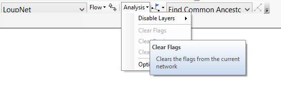
70 Analysis Using a Geometric Network Geometric Network analysis can be used to identify the number of stream links upstream of a point, the total length of the upstream stream links, the total upstream area, drainage density (total length/total area), number of downstream links along path to outlet, and distance to the outlet along the streams. Let s identify one location of interest as a point on the Middle Loup River about ½ way up the basin (see image below), just above the entry of Victoria Creek, a large side tributary. A close-up snapshot of location is below. Zoom to the vicinity of that location (see location below) and place an edge flag using the Utility Network Analyst Add Edge Flag Tool. You may want to add US Topo map to identify the location of interest. If you place the edge flag on a wrong stream, or put more than one edge flag, you can clear the flags located under the Analysis tab of Utility Network Analyst.

71 71

72 72 The above is zoomed in of the Victoria creek confluence with the Middle Loup River. Overlying the topo map. The edge flag is shown as green symbol and it is placed on the Middle Loup above the confluence with Victoria Creek. Notice, that drainage lines do not agree perfectly with the topo map. The topo map is older, but it shows more meandering of the streams which is real and is missed by the steepest descent rule!! This could have serious impact in models that estimate velocities and erosion of streams, transit times, and environment characteristics such as fish habitat (pools and riffles). Please always remember this! You can bookmark this zoomed in view so that you can come back to it later. You can do this by creating the bookmark and giving it a name:

73 73 Now that we placed the edge flag on our location, we can Set the Trace Task to Trace Upstream and press Solve. Next click on the Solve button (see below). The result is a red highlighting of the link that has the edge flag and all links upstream.

74 74 Now we can create a table of segment lengths, etc. in the reaches upstream of our point. Go to Select Analysis and then Options Switch the Results format to Selection. Select Analysis Clear Results and run the trace again.

75 75 Now Open the Attributes table for the DrainageLine (the one with 30,000 threshold) feature and see the selected records Right click on column header Shape_Length and see the Statistics

76 76 These records will differ based on where you put your Edge Flag and in how the various catchments were created (5000 vs etc). Question: Record the total length and number of stream links upstream of your flag. Switch the Trace Task to Trace Downstream and press Solve again. Notice how the selected stream links switch to those downstream from the flag. The following is the view of the entire basin showing downstream of our edge flag highlighted until the outlet.

77 77 Question: Determine the total length of these links as an estimate of the distance along the rivers from your Flag edge to the downstream outlet. Join the Catchment30000 attribute table into the DrainageLine30000 table (operate on the Drainageline feature and click join) using the Grid_Code for a field that join will be based on (see below). This provides access to the area draining directly to each stream link.

78 78 Evaluate the total area upstream of the Flag edge using Shape_Area Statistics. You can also, by placing a flag at an upstream link, determine the flow path (and its length) from any distant link to the outlet. Now, evaluate the length of the longest flow path by choosing a link that appears to have the longest flow path (a bit of trial and error may be necessary) (see screenshot below).

79 79 Prepare a layout that illustrates the longest flow path in the Loup River Basin Turn In: A table and screen shots of an Edge Flag Point for the longest flow line, showing the number of upstream stream links, the total length of upstream stream links, the total upstream area, drainage density (total length/total area), number of downstream links along path to outlet, distance to outlet along the streams. A layout illustrating the longest flow path in the Loup River watershed and giving the length in km. Summary of Items to turn in: PART The number of columns and rows, and grid cell size in the Loup River basin DEM. The minimum and maximum elevation values in the Loup River basin DEM Note the Sum value and the units of the length of the Loup and Middle Loup River from its source to this outlet at Genoa gauge Prepare a layout showing the topography (DEM), Basin Outline, NHDPlusv streams and Loup River Main stem and Middle Loup streams for the Loup River Basin. Include a scale bar and North arrow and appropriate title, labeling and legend so that the map is self-describing. PART 2

80 80 Step 1: The above figure on the left is a closeup of the boxed area in the west central part of the Loup River Basin. That figure, with contours and colorized differences (showing filled pits), may give you a better idea of what these features are. (The circled area is commented on later). o Question: what are these, and should they be filled? Step 3: Turn in the drainage area into the gauge station in both number of 30 m grid cells and as km2 as estimated by the flow accumulation tool. Compare this to the area of the basin, as a check where the area of the basin is obtained from two different sources: a) from the attribute table for the basin, and b) from the USGS properties menu for the Genoa gage as shown below. Also, determine why the Drainage area in the USGS Description has a different value than the contributing drainage area for this particular basin(think about what we have discussed under the flow direction analysis). Step 6: Questions: Compare the two catchment grids (based on 5000 and 30,000 thresholds). Which one appears to present the best representation of catchments for purposes of hydrologic modeling? Justify your answer. Based on the closeups, what are the primary differences between the two catchment maps? Step 7: o Turn in screenshots of the last two figures showing the polygons of catchments and then also with overlays of the stream segment lines. o Describe (with simple illustrations) the relationship between StrLnk, DrainageLine, Catchments and CatchPoly attribute and grid values. What is the unique identifier in each that allows them to be relationally associated? o A layout showing the stream network and catchments attractively symbolized with scale, title and legend. The symbology should depict the stream order for each stream. PART Question: Record the total length and number of stream links upstream of your flag. Question: Determine the total length of these links as an estimate of the distance along the rivers from your Flag edge to the downstream outlet. A table and screen shots of an Edge Flag Point for the longest flow line, showing the number of upstream stream links, the total length of upstream stream links, the total upstream area, drainage density (total length/total area), number of downstream links along path to outlet, distance to outlet along the streams. A layout illustrating the longest flow path in the Loup River watershed and giving the length in km.