AROMAT-I Final Report

Transcription

1 BELGIAN INSTITUTE FOR SPACE AERONOMY AROMAT-I Final Report ESA Study: Airborne Romanian Measurements of Aerosols and Trace gases under contract /15/NL/FF/gp Alexis Merlaud, Mirjam den Hoed, and the AROMAT team The first final report written in the framework of a series of European Space Agency (ESA) field campaigns referred to as AROMAT which were held in Romania in September 2014 (AROMAT-I) and August 2015 (AROMAT-II). AROMAT-I envisaged to test recently developed airborne measurement systems dedicated to air quality research and to explore the possibilities for a larger Sentinel-5 precursor calibration/validation campaign. A full campaign description, data acquisition and analysis, results, two satellite validation dedicated case studies and conclusions are presented in this report. Page 0 of 134

2 Change Log Version Date Status Authors Reason for change Draft Send to Alexis Merlaud M. den Hoed, A. Merlaud New document Draft Send to AROMAT team M. den Hoed, A. Merlaud Updated version Draft Send to ESA and team Hoed, Merlaud, team Completed version Final Send to ESA and team Merlaud, Meier Final Co-authors Name Thomas Wagner (and the MPIC team) Daniel Constantin Andreea Boscarnea Marc Allaart Andreas Meier Anca Nemuc (and the INOE team) Thomas Ruhtz Company MPIC UGAL INCAS KNMI IUP INOE FUB Internal distribution Name Dept Copies For Approval Acceptance Information External distribution Name Company Copies For Approval Acceptance Information Page 1 of 134

3 Table of Content Change Log... 1 Co-authors... 1 Internal distribution... 1 External distribution... 1 List of Acronyms... 6 List of Institutes... 7 List of Participants... 8 Applicable Documents Purpose of the Document Objectives of the AROMAT Activity Objectives for AROMAT-I Objectives for the campaign dataset to serve Instrumental set-up Short overview of the instruments Airborne in-situ Measurements Airborne Remote Sensing Measurements Ground Based Remote Sensing Measurements Ground in-situ Measurements Auxiliary Measurements Unmanned Aerial Vehicle Platforms UAV Flights by RRA and UGAL Flight configuration UAV flights by INCAS Airborne platform Useful satellite instruments and examples of relevant satellite data Ozone Monitoring Instrument METOP AND GOME CALIPSO Overview of the campaign Campaign Time Line Target sites Bucharest Turceni Daily data acquisition tables Page 2 of 134

4 5. Data analysis NO2-sonde (KNMI) Algorithms for the NO2-sonde Precision of the NO2-sonde Parameters received from the radiosonde Aerosol Particle Sizer (APS) SWING (BIRA-IASB) DOAS analysis Georeferencing of the slant columns Conversion to vertical columns Error analysis AirMAP (IUP) Derivation of vertical column densities Results Error analysis Mobile-DOAS (BIRA-IASB) Mobile-DOAS (UGAL) NITROGEN DIOXIDE (NO 2 ) SULPHUR DIOXIDE (SO 2 ) Selected results Mobile-DOAS (MIPC) Spectral Analysis Conversion to VCDs Selected Results Multiwavelength Raman LIDAR (RALI) Data processing procedure Error calculation UV scanning LIDAR (MILI) Data processing procedure Error calculation Aerosol Chemical Speciation Monitor (ACSM) C-ToF Aerosol Mass Spectrometer (AMS) Gas analysers from INOE Gas analysers from UGAL Page 3 of 134

5 5.14 Sun Photometer Aureole and Sun Photometer Data format NO2-sonde, KNMI Aerosol Particle Sizer (APS) SWING (BIRA-IASB) AirMAP (IUP) Mobile-DOAS (BIRA-IASB) Mobile-DOAS (UGAL) Mobile-DOAS (MIPC) Multiwavelength Raman LIDAR (RALI) UV scanning LIDAR (MILI) Aerosol Chemical Speciation Monitor (ACSM) C-ToF Aerosol Mass Spectrometer (AMS) NOx, SO2, CO, O3, THC, AND CO2 Measurements (INOE) NO, NO2 and SO2 Measurements (UGAL) Sun Photometer Bucharest case study Summary of Bucharest measured geophysical parameters Atmospheric trace gases Aerosol properties Analysis of the Golden Day, September 8 th Multiwavelength Raman LIDAR (RALI) Sun photometer-time series data C-ToF Aerosol Mass Spectrometer (AMS) Synergy AirMAP Coincidences with available satellite products Bucharest as location for validation activities OMI overpass at September 8th Simulation for S5P validation Turceni case study Summary of Turceni measured geophysical parameters Atmospheric trace gases Page 4 of 134

6 Aerosol properties Analysis of the Golden Day, September 11 th UV scanning LIDAR (MILI) NO 2 sonde Aerosol Chemical Speciation Monitor (ACSM) Gas analyzers AirMAP SWING Mobile DOAS measurements Synergy Comparison between Magurele and Turceni, September 11th, Coincidences with available satellite products Simulations for S5P validation Summary and lessons learned Acknowledgements References Appendices Summary of retrieved parameters by INOE Additional Airmap measurements in Berlin on AROMAT Data Acquisition Report Page 5 of 134

7 List of Acronyms (MAX-)DOAS ACSM AirMAP AMS APSR AROMAT ASCII ATMOSLAB CCD DOASIS DSCD EARLINET FWHM GPS LOS MILI N/A NMHC NTC OPAMP PBL PC PM10 PPBV PTU QDOAS QGIS RALI RCS SCD SCIATRAN SD SNR or S/N SWING THC UAV UHF UPS UTCC UV VCD (Multi-Axis) Differential Optical Absorption Spectroscopy Aerosol Chemical Speciation Monitor Airborne imaging DOAS instrument for Measurements of Atmospheric Pollution Aerosol Mass Spectrometer Aerodynamic Particle Sizer Spectrometer Airborne Romanian Measurements of Aerosols and Trace gases American Standard Code for Information Interchange Airborne Laboratory based on Hawker Beechcraft Charge-Coupled Device DOAS Intelligent System: all-round tool for working with spectral data Differential Slant Column Densities European Aerosol Research LIDAR Network Full Width at Half Maximum Global Positioning System Lines Of Sight Eye-safe UV scanning LIDAR Not Applicable NonMethane HydroCarbons Negative Temperature Coefficient (thermistor) OPerational AMPlifier Planetary Boundary Layer Personal Computer Particulate Matter up to 10 micrometres in size Parts Per Billion by Volume Pressure, Temperature, and humidity (sensor) User interface dedicated to the DOAS retrieval of trace gases Cross-platform, free, open source desktop Geographical Information System Multiwavelength depolarization Raman LIDAR Range Corrected Signal Slant Column Density Software package with radiative transfer model and retrieval algorithm Secure Digital Signal-to-Noise Ratio Small Whiskbroom Imager for trace gases monitoring Total HydroCarbons Unmanned Aerial Vehicle Ultra High Frequency Uninterruptible Power Supply Coordinated Universal Time Ultra Violet Vertical Column Density Page 6 of 134

8 List of Institutes The institutes presented below have participated in the AROMAT campaign and have contributed to its scientific purposes by performance of the following task(s): European Space Agency (ESA): Mission leader and funder. The Belgian Institute for Space Aeronomy (BIRA-IASB): Played the principal role in campaign organization and has performed both measurements with the self-developed SWING instrument mounted on a UAV [p. 28], and with a mobile-doas instrument mounted on a car [p. 36]. The Royal Netherlands Meteorological Institute (KNMI): Contributed substantial to the campaign organization and has flown self-developed NO2-sondes under a meteorological balloon as well as on a UAV [p.13]. The Dunarea de Jos University of Galati (UGAL): Substantially Contributed to the campaign organization and has conducted both mobile-doas car measurements [p. 41] and in-situ trace gas measurements from a mobile lab [p. 56]. The National R&D Institute for Optoelectronics (INOE): Substantially Contributed to the campaign organization, and has performed an extensive series of ground measurements: LIDAR [p. 47], aerosol [p.59], trace gas [p. 63], and auxiliary measurements [p. 67]. Also an Aerodynamic Particle Sizer Spectrometer was operated on board of a UAV [p. 22]. The Institute of Environmental Physics Bremen (IUP): Conducted airborne measurements with the self-developed AirMAP instrument on board of a Cessna research aircraft [p. 32]. The National Institute of Aerospace Research ELIE CARAFOLI (INCAS): Built and operated a large beach-craft type research UAV and operated from it a commercial aerosol particle sizer [p. 22]. The Max Planck Institute for Chemistry (MPIC): Performed car-max-doas measurements throughout the campaign [p. 44]. The Free University of Berlin (FUB): Operated their Cessna P207 research aircraft and conducted both handheld sun photometer and airborne measurements [p. 71]. Reev River Aerospace (RRA): Operated all UAV flights performed in Turceni and built the two UAV s deployed at that location [p. 16]. The National Institute of Aerospace Research ELIE CARAFOLI (INCAS): Built and operated a large research UAV equipped with a commercial aerodynamic particle sizer [p. 22]. Page 7 of 134

9 List of Participants The following participants have committed themselves for the benefit of the good results achieved during the first AROMAT campaign: Name Alexis Merlaud Frederik Tack Michel Van Roozendael Dirk Schuettemeyer Paul Ingmann Thomas Ruhtz Carsten Lindemann Andreea Boscornea Visoiu Constantin Sorin Vajaiac Paula Mursa Andre Seyler Anca Nemuc Cristian Radu Doina Nicolae Andreas Richter Anja Schoenhardt Andreas Meier Mirjam den Hoed Marc Allaart Piet Stammes Thomas Wagner Reza Shaiganfar Katharina Riffel Sebastian Donner Florin Mingireanu Ionut Mocanu Daniel Constantin Carmelia Dragomir Marius Bodor Lucian Georgescu Institute BIRA BIRA BIRA ESA ESA FUB FUB INCAS INCAS INCAS INCAS INOE INOE INOE INOE IUP IUP IUP KNMI KNMI KNMI MPIC MPIC MPIC MPIC ROSA RRA UGAL UGAL UGAL UGAL Page 8 of 134

10 Applicable Documents Type Author Company Reference Statement of Work Dirk Schuettemeyer ESA EOP-SM/2625/DS-ds Campaign Implementation Plan Alexis Merlaud BIRA AROMAT-CIP-1 Data Acquisition Report Mirjam den Hoed KNMI AROMAT-DAR-1 1. Purpose of the Document The purpose of this document is to provide a complete description of all the work done during the first ESA study titled Airborne ROmanian Measurements of Aerosols and Trace gases (AROMAT-I), which was held on two sites in Romania in September It provides a comprehensive overview of the campaign including its context and objectives, a description of the instrumental set-up, the activities performed and the main results achieved. Also the applied methods for data unpacking, formatting and calibration, data quality analysis and data processing for scientific analysis and the generation of data products is described. Furthermore, examples of processed data are provided in the form of an in-depth data analysis for the two measurement sites Bucharest and Turceni, describing the measured geophysical parameters and presenting comparisons with available satellite products including simulations for Sentinel-5-precursor (S5p) validation. Lastly the lessons learned during AROMAT-I are presented to be taken into account during follow-up activities and future campaigns in the framework of AROMAT and/or in Romania. Page 9 of 134

11 2. Objectives of the AROMAT Activity The overall objectives of AROMAT were derived from the general scientific objectives of several upcoming European Space Agency (ESA) missions in the context of future Earth Observation (EO) programmes and their user community. In addition the objectives were relevant for validation campaigns, which are prepared and conducted as part of current satellite missions, in orbit or under development like the Copernicus Sentinel-4/-5 missions. Such campaigns provide feedback on key issues related to the definition, performance and product quality of different remotely sensed and in-situ species monitored by satellite instruments. 2.2 Objectives for AROMAT-I The main objective of this first AROMAT campaign was to test newly developed airborne sensors and to evaluate their capabilities as validation tools for future air quality space borne sensors, in particular TROPOMI. At the same time the recent trend to develop compact sensors was taken into account since these would also fit on board smaller aircraft and even current state of the art UAVs. Typical examples of compact sensor developments at the time were the AirMAP instrument developed by the University of Bremen in Germany, the SWING instrument developed by BIRA in Belgium, and the NO2-sonde developed by KNMI in the Netherlands (chapter a, a, b and appendix I). These three recently developed airborne instruments dedicated to NO 2 monitoring have been operated quasi-simultaneously during the second Turceni phase, also referred to as phase B of the campaign, when the AROMAT measurements concentrated on one of the large thermal plants in the Jiu Valley (figure 1, location B). Their airborne measurements would yield simultaneously recorded NO 2 vertical columns from AirMAP and SWING, and NO 2 vertical profiles from the NO2-sonde. In addition to these airborne sensors, ground-based measurements were conducted to provide valuable complementary geophysical data. From LIDAR measurements aerosol extinction profiles would be obtained as well as the dynamics of the atmosphere. In-situ measurements would indicate the ground level of NO 2 and of several other species relevant for air quality research, such as SO 2 and carbon monoxide (CO). Furthermore, mobile-doas measurements revealed the vertical columns of NO 2 and SO 2 along the roads in the vicinity of the plant. Page 10 of 134

12 Figure 1: NO 2 map of Romania derived from OMI data. The two targets of the AROMAT campaign are labeled A (Bucharest) and B (Turceni-Rovinari power plants) (Adapted from Constantin et al., 2013) The AROMAT experiment took advantage of the high NO 2, SO 2, and aerosol levels and gradients in the Turceni area to investigate the consistency and the complementarity of the different measurement approaches, e.g. comparing the maps derived from AirMAP and SWING, or introducing the NO2-sonde and LIDAR profile information in the column measurements from AirMap, SWING, and mobile DOAS. Combining the information from the NO 2 vertical columns measured from ground level upwards by the mobile DOAS systems to those measured from a known altitude downwards by AirMAP and SWING would reveal valuable information about the NO 2 vertical profile shape (e.g. the actual height of the NO 2 ), which can be compared to the NO 2 vertical profiles measured by the NO2-sonde. The experiment addressed various geophysical questions: What are the NO 2, SO 2 and aerosol levels and vertical distributions upwind and downwind of the plants? What is the spatial extent and the shape of the exhaust plume? How are these quantities correlated? What are the diurnal variations of these species in this area in summer? What is the diurnal evolution of the boundary layer height? In the context of satellite validation studies, the measurements would provide information on the NO 2 variability within part of a virtual S5p swath by covering several of the envisaged seven by seven kilometre pixels within a short time interval. The NO 2 vertical profiles measured with the NO 2 -sonde were to be included in the satellite retrievals to investigate the effect of these profiles on the tropospheric satellite products. The scientific objectives of the Bucharest (figure 1, location A) phase, also referred to as phase A of the AROMAT campaign, were similar to the Turceni phase, however without the UAV and balloon flights, since flight clearances for unmanned platforms are an issue over this populated area. The dataset of Bucharest would yield insights on the typical pollution levels around and across the city in summer, the time variations of the species and their spatial gradients. Noteworthy is that a ring road Page 11 of 134

13 motorway enabled the team to perform full circles around the city with mobile-doas instruments. Using accurate wind data, it would be possible to derive the total NO 2 flux from Bucharest, as was already done for several large cities with similar systems. All these geophysical information will be valuable to prepare the 2017 larger TROPOMI calibration and validation campaign in the Bucharest area, but AROMAT will also be useful as a precursor campaign from a logistics and administrative point of view. 2.3 Objectives for the campaign dataset to serve In summary, the campaign dataset was intended to serve the following objectives: Verification of different sensor s performances using airborne measurement activities. Through this activity, it would be possible to verify that their measured signals are suitable for observation from space in the context of future missions, and support the elaboration of mission-specific algorithms, Assessment of 3-dimensional variability of different species in the atmosphere utilising state of the art retrieval techniques Provision of a basis for the quantitative assessment of current existing satellite data also taking heterogeneous scenes into account Verification of the overall concept as an airborne support activity to Earth Explorer and Copernicus missions. Page 12 of 134

14 3. Instrumental set-up During AROMAT-I three recently developed airborne instruments dedicated to NO 2 monitoring (AirMAP from IUP, the NO 2 -sonde from KNMI, and SWING from BIRA) were operated, respectively from the FUB Cessna, weather balloons, and an Unmanned Aerial Vehicle (UAV) of UGAL. Commercial aerosol particle sizers were also used onboard an INCAS UAV. These airborne measurements were performed in coincidence with measurements conducted with ground-based instruments, such as NO x, SO 2, CO and Ozone (O3) in-situ gas analyzers from INOE and UGAL, 2 LIDARs from INOE and four mobile-doas systems from UGAL, MPIC and BIRA. The latter can also detect SO 2 and H 2 CO, which are mandatory products for TROPOMI/S5p. Paragraph 3.1 gives a short description of all instruments mentioned, while an extensive overview of the instrumental set-up can be found in the Data Acquisition Report (DAR) (Appendix I). In paragraph 3.2 an overview is given of satellite instruments currently in orbit, from which relevant data can be retrieved to test the validation capabilities of the AROMAT-I measurement approach. 3.1 Short overview of the instruments Airborne in-situ Measurements a NO2-sonde The KNMI NO 2 -sonde has been measuring 13 vertical NO 2 -profiles, 11 flying under a meteorological balloon and 2 flying on a UAV platform. The NO 2 sensor s measurement principle is based upon the chemical reaction between Nitrogen dioxide and luminol, a chemiluminescent reaction that produces a faint blue light. The reaction chamber contains luminol dissolved in (alkaline) water. Ambient air is pumped through a Teflon pump, and bubbled through the sensing solution. The light that is produced by the reaction is detected by an array of photodiodes that is glued to the reaction chamber. The electric current from the photodiodes is converted into a voltage with a highly sensitive operational amplifier (OPAMP), and passed through a filter that removes high frequency fluctuations. The NO 2 -sonde, when operated under a meteorological balloon, consists of 2 parts: the NO2-sensor that was developed at KNMI, and a commercial radiosonde. In this document the algorithms used to derive NO 2 from the NO 2 -sonde, the expected precision of its results, and the expected precision of the radiosonde are discussed in section 5.1. Please note that the inner workings of the radiosonde are not described, as this is a commercial instrument. Page 13 of 134

15 Figure 2 (left): NO2-sonde + radiosonde before launch in Turceni. Figure 3 (right): Close-up of the NO2-sensor, which during operation resides inside of the Styrofoam box b Aerosol Particle Sizer Spectrometer (APS) Location of measurements: Clinceni, Ilfov (44.358N E) The instrument was installed on the INCAS UAV and flown over Clinceni area up to 1.1km. Measurement principle: The Aerodynamic Particle Sizer provides the diameter of particles using time-of-flight technique on μm particles, measured in an accelerating flow field with a single high speed timing processor. Simultaneously, a light scattering technique is used to detect particles between 0.37 and 20 μm. The Aerodynamic Particle Sizer Spectrometer can measure from 0.5 to 20 μm by aerodynamic sizing and 0.37 to 20 µm by optical detection. Known issues: the sampling module from the UAV was somehow basic and the high size particles could be obstructed, leading sometimes to erroneous data readings. Species measured: aerosol size distribution in number, volume and mass weight units. Parameters delivered: PM1, PM2.5, PM10, TSP, aerosol size distribution Airborne Remote Sensing Measurements a SWING onboard the Uni. Galati UAV The SWING payload is a whiskbroom imaging system developed at BIRA in collaboration with UGAL and designed to be operated from an Unmanned Aerial Vehicle (UAV) [RD-1]. The instrument is based on an AVANTES compact ultra-violet visible spectrometer and a scanner to achieve whiskbroom imaging of the trace gases fields. Including the housing and the electronics, the weight, size, and power consumption of the SWING payload are respectively 1200 g, 33x12x8cm 3, and 10 W. Page 14 of 134

16 Figure 4: SWING mounted on UGAL UAV at UAV airfield 1.3 km NNW of the Turceni power station. Figure 5: Overview of the SWING instrument components b AirMAP The Airborne imaging Differential Optical Absorption Spectroscopy (DOAS) instrument for Measurements of Atmospheric Pollution (AirMAP) has been developed for the purpose of trace gas measurements and pollution mapping. The instrument was operated on the FUB Cessna 207 Turbo aircraft. The AirMAP is a push-broom UV/vis imager with a wide field-of-view of around 51 across track, leading to a swath width of about the same size as the flight altitude. Due to its large swath and the use of a frame transfer charge coupled device (FT-CCD) detector, gapless maps of horizontal Page 15 of 134

17 trace gas distributions can be acquired within a relatively short time. For example with the AirMAP setup it is possible to examine the sub-pixel variability within one OMI (Ozone Monitoring Experiment) pixel (13x24 km at nadir) in a time window of less than one hour with ground spatial resolutions below 100 m at a typical flight altitude of 3.2 km. Figure 6: Sketch of AirMAP s instrumental setup, (Schönhardt et al. 2015). Figure 7: AirMAP's observation geometry adapted from (Schönhardt et al. 2015). The instrumental setup and the viewing geometry are shown in Figure 6 and Figure 7, respectively. Scattered sunlight from below the aircraft is collected with a wide field of view objective. The light is coupled into an imaging grating spectrograph via a sorted fiber bundle, retaining the spatial information. The dispersed light is imaged onto a FT-CCD. The CCD images are stored on a PC. From a maximum of 35 individual viewing directions, represented by 35 single fibers, the number of viewing directions can be adapted to each situation by averaging according to signal-to-noise or spatial resolution requirements. The single fibers are stacked vertically at the spectrometer entrance Page 16 of 134

18 slit and are oriented across flight direction in the focal point of the telescope. The spectrometer is an Acton 300i imaging spectrograph with a focal length of 300 mm, and an f-number of f/3.9. The wavelength region can be chosen according to the chemical species of interest, with a spectral coverage of 41 nm or 86 nm, using a 600 g/mm grating blazed at 500 nm or a 300 g/mm grating blazed at 300 nm, respectively. During the AROMAT campaign the 600 g/mm grating was used for measurements in the visible spectral range ( nm). The 300 g/mm grating was used for measurements in the UV ( nm). The spectrometer is temperature stabilized at 35 C. The frame transfer technique of the CCD provides a fast frame rate, because the electrons are quickly shifted into a second storage area for read-out. This allows gapless measurements, because the next image can be recorded within milliseconds. For data safety reasons, the CCD readout is interrupted and restarted every few minutes resulting in small measurement gaps. The instrument is further equipped with an optional camera for scene photography. These photographic images are triggered by the spectroscopic measurements and can be used, e.g., for position control and interpretation of the observed scene. The AirMAP instrument as well as the aircraft is equipped with an Attitude and Heading Reference System (AHRS) and GPS sensor. The instrument measures spectra of scattered sunlight. The spectra are analyzed using Differential Optical Absorption Spectroscopy (DOAS) in order to derive column densities of trace gases. A detailed description of the instrumental setup, its performance, the viewing geometry and the georeferencing is described in (Schönhardt et al. 2015) Ground Based Remote Sensing Measurements a Mobile-DOAS from BIRA-IASB The BIRA double channel mobile-doas instrument is based on a double channel Avantes spectrometer installed on a car. The spectral range is nm with a 1.2 nm resolution (FWHM). An optical head, mounted on the car window, holds the two telescopes achieving a 2.5 field-of-view with fused silica collimating lenses. One telescope points zenith while the other is directed 30 above the horizon. Two 400 µm chrome plated brass optical fibers connects the telescopes to the spectrometer. Page 17 of 134

19 Figure 8: Measurement of NO 2 in Turceni during AROMAT with the BIRA Mobile DOAS system (the optical head is visible on the window) b Mobile-DOAS from UGAL "Dunarea de Jos University" of Galati was involved in AROMAT-1 campaign with zenith-sky mobile DOAS observations. Using the zenith-sky mobile DOAS system UGAL was able to determine the tropospheric NO 2 and SO 2 amount along the route of measurements around Bucuresti and Turceni. In Figure 9 is presented the mobile DOAS system used by UGAL during AROMAT-1. Figure 9: The mobile DOAS system (sketch and artistic photo). The mobile DOAS instrument used for AROMAT measurements is based on a compact Czerny-Turner spectrometer (AvaSpec-ULS2048XL-USB2, of mm dimensions and 855 g weight) placed in a car. The spectral range of the spectrometer is nm with 0.7 nm resolution (FWHM) with a focal length of 75 mm. The entry slit is 50 μm and the grating is 1200 L/mm, blazed at 250 nm. A flexible device (a piece of wood with a hole cached in a small metallic plate), mounted Page 18 of 134

20 on the top of the road vehicle, holds the telescope achieving a 1.2 field-of-view with fused silica collimating lenses. The spectrometer is connected to the telescope through a 400 μm chrome plated brass optical fiber. Each spectrum is recorded by a laptop and georeferenced by a GPS receiver. The spectrometer and the GPS receiver are powered by the laptop USB ports. The entire set-up is powered by 12 V of the car through an inverter. Each measurement is a 10-second average of 10 scans accumulations at an integration time between ms. All observations were performed only in zenith geometry c Mobile-DOAS from MPIC The MPIC team used two Mini-MAX-DOAS instruments mounted on the roof of a car. One instrument covered the UV and blue spectral range and was directed in backward direction. The second instrument covered the visible spectral range and was directed in forward direction (see Fig. 10). A summary of the instrumental properties and the measurements strategies is given in Table 1. The temporal coverage of successful measurements of both instruments is provided in Table 1. Figure 10: Two Mini-MAX-DOAS instruments mounted on the roof of the car. Property UV-instrument Vis-instrument Spectral range nm nm Spectral resolution nm nm Typical integration time 30 or 60 sec 30 sec Viewing direction 90 and 22 backward 90 and 22 forward Table 1: Instrumental properties and measurement strategies of both Mini-MAX-DOAS instruments d Multiwavelength Raman LIDAR (RALI) Location of measurements: Magurele, Ilfov (44.35 N, E) Measurement principle: elastic backscattering of the laser light (1064, 532 and 355nm) by the molecules and aerosols in the atmosphere Page 19 of 134

21 Known issues: the overlap of the LIDAR is above 500m; layers near to the ground cannot be quantitatively assessed; information extracted from the LIDAR describes generally long-range transport of particles, i.e. in the free troposphere Species measured: aerosols Parameters delivered: 1-h averaged backscatter and extinction vertical profiles (cloud screened) 5-min. averaged PBL height e UV scanning LIDAR (MILI) Location of measurements: Turceni, Gorj (44.66N, E) Measurement principle: elastic backscattering of the laser light (355nm) by the molecules and aerosols in the atmosphere Known issues: the overlap of the LIDAR is above 200m; layers near to the ground cannot be quantitatively assessed; information extracted from the LIDAR describes generally long-range transport of particles, i.e. in the free troposphere Species measured: aerosols Parameters delivered: 1-h averaged backscatter and extinction vertical profiles (cloud screened) 5-min. averaged PBL height Ground in-situ Measurements a Aerosol Chemical Speciation Monitor (ACSM) Location of measurements: Turceni, Gorj (44.66N, E) Measurement principle: sampled submicronic aerosols are vaporized and detected by an electron impact quadrupole mass spectrometer; an automated zeroing system is implemented, using the naphthalene filter (Ng et al., 2011; Petit et al., 2015). Known issues: the ACSM uses sampling technique near to the ground; information extracted from this instrument generally describes locally-produced aerosols; in some particular meteorological conditions, particles from elevated layers may reach the ground and be sampled by the ACSM Species measured: aerosols Parameters delivered: 30 min average mass concentrations of particulate Organics, Sulfate, Nitrate, Ammonium and Chloride Page 20 of 134

22 3.1.4.b C-ToF Aerosol Mass Spectrometer (AMS) Location of measurements: Magurele, Ilfov (44.35 N, E) Measurement principle: mass spectrometry implies the submicronic aerosols vaporization and conversion to positive ions, which can then be detected by the mass spectrometer; particle aerodynamic diameter is determined from particle time-of-flight velocity measurements using a beam -chopping technique (Jayne et al., 2000). Known issues: the C-ToF AMS uses sampling technique near to the ground; information extracted from this instrument generally describes locally-produced aerosols; in some particular meteorological conditions, particles from elevated layers may reach the ground and be sampled by the C-ToF AMS (Nicolae et al., 2013). Species measured: aerosols Parameters delivered: mass concentration time series for several species aerosols: organics, nitrate, sulphate, ammonium, chloride vacuum aerodynamic size distribution of submicronic aerosols c Gas analysers from INOE Location of measurements: Turceni, Gorj (44.679N, E) Measurement principle: The gas analyzers measure gas concentrations using classical methods such as the cross-flow modulated semi decompression chemoluminiscence method (for NO x monitor), UV fluorescence (SO 2 monitor), non-dispersion cross modulation infrared analysis method (CO monitor), ultraviolet absorption method (O 3 monitor), cross-flow modulated selective combustion type method combined with a hydrogen ion detection method (THC monitor) and gas filter correlation spectroscopy (CO 2 ). Known issues: The instruments require periodic zero/span calibrations to ensure the quality of the data. Another issue that could affect the data is related to the instrument response time. According to the measured species, the gas analyzers have different response times related to the measurement principle. For the CO monitor, the response time is within 50 seconds at the lowest range (LR), the SO 2 monitor has a response time within 120 seconds LR, the NO 2, NO monitor has a response of 90 seconds LR, for the THC monitor the response time is within 60 seconds and the time response for the ozone monitor is 75 seconds. These response times can affect fast changing concentrations of ambient gas detected by the instrument. Species measured: CO (0-100ppm), SO 2 (0-0.5ppm), NO, NO 2 (0-1ppm),CH 4, NMHC, THC (0-50ppmC), O 3 (0-1ppm) Parameters delivered: The primary parameter measured by the instrument is the concentration of one or several gas species within the ppb-ppm range. Page 21 of 134

23 3.1.4.d Gas analysers from UGAL "Dunarea de Jos University" of Galati was involved in AROMAT-I campaign with in-situ measurements using a mobile laboratory, which was used in both locations, Bucharest and Turceni. The main instruments operated from this mobile lab were: UV Fluorescence Sulfur Dioxide (SO 2 ) analyzer, Model: AF22M; Chemiluminescent Nitrogen Oxides Analyzer (NO/NO 2 /NOx - NH3), Model AC32M; Calibrator (Model: LNI); Weather station (wind speed, temperature, relative humidty, solar radiation, precipitation, and atmospheric pressure); System for data acquisition and digital processing. Figure 11: The mobile in-situ laboratory of UGAL e Sun Photometer (INOE) Location of measurements: Magurele, Ilfov (44.35 N, E) Measurement principle: direct sun measurements at eight spectral bands: 340, 380, 440, 500, 670, 870, and 1020 nm. The instrument is part of the Aerosol Robotic Network (AERONET) and the data is available online. Known issues: parameters are retrieved for the atmospheric column; the output includes both retrieved aerosol parameters and calculated on the basis of the retrieved aerosol properties (Dubovik and King, 2000); the volume particle size distribution dv(r)/dlnr (μm3/μm2) is retrieved in 22 logarithmically equidistant bins in the range of sizes 0.05μm r 15 μm (Dubovik et al., 2000). Species measured: aerosols Parameters delivered: AOD (550nm), Angstrom exponent ( nm), size distribution, fine mode fraction Page 22 of 134

24 3.1.5 Auxiliary Measurements During the AROMAT campaign auxiliary measurements have been conducted, measuring not the by AROMAT targeted aerosols and trace gases, but other geophysical constants like sun radiance, sky radiance and weather conditions a Weather Station (INOE) On the rooftop of the INOE minivan a weather station was installed measuring the following meteorological parameters contained in the Weather station directory : station name, date, time, rain data, wind direction, wind speed, pressure, relative humidity and temperature b Microtops II: Technical Description: The handheld Sun photometer manufactured by SOLAR LIGHT and owned by the Freie Universität Berlin offers five channels with different narrow spectral filters at 380nm, 500nm, 870nm, 936nm (for columnar water vapor retrieval) and 1020nm. The instruments provides the operator a Sun target screen to enable accurate pointing of the instrument at the sun. The Microtops is connected to a Garmin GPS 72H device by a serial data cable to provide position and UTC time of each scan. In the settings required by the GSFC for AERONET processing, the instrument does 20 scans within approximately 8 seconds and only stores the data from the scan with the highest signal. The Data acquisition was performed on ground during AROMAT-1 flight operations at the Baneasa Airport and was processed by the standard microtops software. Figure 12: Microtops-II (left), and MT-II results of September 2 nd and September 9 th respectively in Bucharest (middle and right) c Aureole & Sun Adapter 2 The airborne spectrometer system FUBISS-ASA2 provides simultaneous measurements of the direct solar irradiance and the aureole radiance in two different solid angles. The high resolution spectral radiation measurements are used to derive vertical profiles of aerosol optical properties. Combined measurements in two solid angles provide better information about the aerosol type without additional and elaborated measuring geometries. It is even possible to discriminate between absorbing and non-absorbing aerosol types. Furthermore, they allow to apply additional calibration methods and simplify the detection of contaminated data (e.g. by thin cirrus clouds). For the characterization of the detected aerosol type a new index is introduced which is the slope of the Page 23 of 134

25 aerosol phase function in the forward scattering region. The instrumentation is a flexible modular setup, which has already been successfully applied in airborne and ground-based field campaigns. Technical data FUBISS-ASA2 Spectral range (usable) [nm] Spectral resolution (FWHM) 10 [nm] Spectral pixel distance 3.3 [nm] Number of channels 256 Field of View Direct 1,5 [ ] Aureole I 4 ± 0.85 [ ] Aureole II 6 ± 0.96 [ ] pointing accuracy < 0.1 [ ] Typical measurement time for single spectra Direct (clear Atmosphere) (turbid Atmosphere) Aureole (clear Atmosphere) (turbid Atmosphere) Dynamic range 15 [bit] Table 2: Technical data from FUBISS-ASA1 and FUBISS-ASA2. [ms] [ms] Figure 13: Aircraft installation of FUBISS-ASA2(left) and its measurement principle illustrated (right) d Cessna 207T Navigation System (IGI AEROcontrol) AEROcontrol is IGI's GPS/IMU system for the precise determination of position and attitude of an airborne sensor. This can be the position of the projection center and the angles omega, phi, kappa of the aerial camera system or an airborne laser scanner. The AEROcontrol system consists of an Inertial Measurement Unit (IMU-IIe) based on fibre-optic gyros (FOG) and a Sensor Management Unit (SMU) with integrated high end GPS receiver. Page 24 of 134

26 AEROcontrol can be operated either as a stand-alone system or combined with other Sensor Management Units via its Ethernet interface. Because of its modular design, the AEROcontrol SMU can be adapted to customer needs easily. The SMU can manage three different events (eg. trigger for camera or real-time data) and one IMU input. (Ref.: The data processing can be performed in three steps. The first mandatory step performed by the AEROoffice pre-processing software gives already position and attitude information in medium quality. An optional step can be a differential GPS correction by the Inertial explorer software of the GPS manufacturer Novatel. The last step of the AEROoffice post-processing software merges the results into an inertial closure with higher accuracy and error information e Complementary Data The European Center for Medium range Weather Forecasting (ECMWF) forecast model PBL height was used to compare the similar product from LIDAR (Dee et al.,2011). The MODIS AOD(Levy et al.,2015) was used to constrain the LIDAR extinction profile in Turceni, and to compare the 2 locations. HYSPLIT backtrajectories (Draxler et al, 2014) were used to estimate the source and paths of the aerosol layers reaching the 2 locations at the altitudes measured by the LIDARs. 3.2 Unmanned Aerial Vehicle Platforms During the AROMAT-I campaign two so-called Unmanned Aerial Vehicles were used from which the ASPR, SWING and the NO 2 -sonde were operated UAV Flights by RRA and UGAL The Uni. Galati UAV was used in the Turceni phase of the campaign and performed flights with the SWING instrument or the NO 2 sonde. Figure 14: UAV of the University of Galati, developed by Reev River Aerospace Page 25 of 134

27 This Uni. Galati UAV was developed and operated during the campaign by Reev River Aerospace. It has a 2.5 m wingspan, it is electrically propelled and typically fly at 100 km/h. The autonomy is 1h30 and it can reach an altitude of 3 km in autopilot. Figure 15: Three of the UGAL UAV flight paths in Turceni (10 and 11 September 2014) Figure 15 shows three of the SWING flights performed with the Uni. Galati UAV during the AROMAT campaign. They were performed in visual range and the UAV reached an altitude of 600 m above the ground Flight configuration UAV flights by INCAS Figure 16: INCAS unmanned airborne platform. Page 26 of 134

28 INCAS owns under the nomenclature ATMOSLAB a fully operational airborne laboratory, a ground mobile laboratory and a parallel computing system and a large scale UAV. The available UAV was built as a 1:3 scale model of a conceptual passenger aircraft for the validation of the designed flight characteristics, and was used used for mounting the INOE ASPR sensor system. The UAV platform was equipped with a Nelsn Hobbysi control system, that is formed by a SMARTFLY board personally customized main-board, which guarantees the necessary redundancy to ensure the process of flight in optimal conditions. Furthermore it has a 3W-275XiB2 TS / CS engine, which is based on two cylinders with a cylinder capacity of 150 m 3. Other specifications are: Propulsion System: 3W-275cc, Wingspan: 21 ft. (252 ), Length: 14 ft. (168 ), Flying Weight: 115 pounds and Height: 50. Figure 17: UAV flight paths of performed during AROMAT-1 campaign , first and second flight. During the flights performed under AROMAT-1 campaign the UAV platform was equipped with a commercial Aerodynamic Particle Sizer (TSI Instruments). The selected research area was the Bucharest metropolitan area, more specific at about 20 km South-West of the city (around Clinceni area). Some flight paths followed during the research campaign (performed on ) are presented in Figure Airborne platform FUB Cessna 207T The aircraft used in this experiment was a single engine Cessna 207T. The aircraft can be equipped with multiple instruments with a maximum instrument weight of up to 300 kg. It has three downward and one sideward looking opening. The instruments can be mounted on the cabin floor with mechanical adapters or in an 19 Rack. Each modification to an aircraft has to pass a certification program. The FUB Institute for space sciences is certified (LBA.21J.0023) by the Luftfahrtbundesamt (LBA) to design changes to aircraft specifically designed and modified for research or scientific purposes (pursuant Regulation (EC) No 1592/2002, Article 4(2) and Annex II (b), corresponding JAR-21, Subpart E) in accordance with the applicable airworthiness requirements. The instrumentation and all requirements to modify the existing aircraft were certified in accordance to the previews rules. Page 27 of 134

29 Table 3: CESSNA 207 T aircraft technical data. Figure 18: FUB Cessna 207T. Page 28 of 134

30 Figure 19: AROMAT-1 FUB Cessna 207T navigation data results: Overview of flights. 3.3 Useful satellite instruments and examples of relevant satellite data The Ozone Monitoring Instrument (OMI), the Global Ozone Monitoring Experiment-2 (GOME-2), and the Cloud-Aerosol LIDAR and Infrared Pathfinder Satellite Observation (CALIPSO) are examples satellite instruments making use of remote sensing the observation from a distance monitoring the earth and its atmosphere from space using a variety of techniques. These three satellite instruments currently in orbit, produce relevant data from the composition of the earth s atmosphere (O 3 vertical profiles, accurate information on the total column amount of NO 2, SO 2, water vapour, oxygen/oxygen dimmer, bromine oxide, aerosol characterization) and cloud coverage on a daily basis. AROMAT data, airborne as well as ground-based, can be used to validate the geophysical parameters measured by these instruments, quantifies using state of the art retrieval techniques and algorithms. The instrumental and experimental set-up of AROMAT should yield a better characterization of 3-dimensional variability of different species, which is a major limiting factor for satellite validation. In this paragraph three satellite instruments are described that currently produce relevant data that could be validated using data from AROMAT. Page 29 of 134

31 3.3.1 Ozone Monitoring Instrument OMI is a nadir viewing imaging spectrograph that measures the solar radiation backscattered by the Earth's atmosphere and surface over the entire wavelength range from 270 to 500 nm with a spectral resolution of about 0.5 nm. The instrument is situated on board of the EOS-AURA satellite from the American Space Agency NASA. It takes this satellite 98 minutes to complete its orbit around the earth imaging a 2600 kilometer wide strip with every orbit. After fourteen orbits which are being traveled within a day, the entire planet earth has been covered. In the normal global operation mode, the OMI pixel size is 13 km 24 km at nadir (along x across track). In the zoom mode the spatial resolution can be reduced to 13 km 12 km. The small pixel size enables OMI to look in between the clouds, which is very important for retrieving tropospheric information. Usage of a two-dimensional detector makes it possible to measure the complete spectrum in the ultraviolet/visible/near-infrared wavelength range, which enables one to retrieve several trace gases from the same spectral measurement, combined with a very high spatial resolution and daily global coverage. The instrument accurately measures the extend of air pollution (NO 2, SO 2, soot, particulate matter (PM) and volcanic ash) in different cities worldwide and how it travels. This enables one to map large-scale air pollution transport like from the United States (US) to Europe and from China to the US. The data is used to generate air quality forecasts and to issue volcanic ash warnings. Moreover, the thickness of the Ozone layer is measured to the smallest detail, which is important for climate change and greenhouse effect studies, as well as for human health. The Ozone layer filters the Ultraviolet (UV) radiation that is harmful for human skin. Too much exposure to UV can lead to the formation of skin cancer. Partly due to changeable weather conditions, the thickness of the Ozone layer varies, causing the natural filter to work better one day than the other. By means of OMI UV forecasts can be made one week ahead for the entire world. OMI enables both policy makers and scientists to measure to what extend the measures taken to limit depletion of the Ozone layer are having the desired effect. OMI Standard Data products include Level-1b data, the O3 total column, the O3 vertical profile, Cloud Pressure and Fraction, Surface UVB flux, the HCHO total column, the BrO total column, the OClO slant column, surface Reflectance, the OMI slit function and most important for the AROMAT-I campaign the NO2 total and tropospheric column, the SO2 total column and Aerosol. Page 30 of 134

32 Figure 20: Vertical Columnar Density of SO 2 in Dobson Units, measured by OMI in Romania between 2005 and From the TEMIS website ( files containing OMI NO 2 data for individual orbits can be downloaded..tar files are compressed files and once they are unpacked, can be opened in a free software program called Panoply. Panoply can be used to explore all level 2 data fields associated with the OMI Level 2 DOMINO NO 2 retrieval including cloud cover error characteristics and geo location fields. OMI measures a tropospheric and total vertical column of NO 2. The following 3 figures show data fields collected by OMI. From these multiple data fields the NO 2 levels can then be zoomed in to identify the pixels corresponding to Bucharest and Turceni. Figure 21 (left): Panoply generated DOMINO NO 2 plot that shows the tropospheric vertical column density for the 8 th of September for the particular orbit that passes Romania. Figure 17 (right): TEMIS generated plot of the NO 2 tropospheric vertical column averaged over September 2014 for Europe measured by OMI. Page 31 of 134

33 The OMI data can be visualised in more detail with the Geospatial Interactive Online Visualization ANd analysis Infrastructure (GIOVANNI), a web-based application developed by the NASA Goddard Earth Sciences Data and Information Services Center (GES DISC) that provides a simple way to visualize, analyze, and access vast amounts of earth science remote sensing data without having to download the data, and by the TEMIS website. GIOVANNI and TEMIS can be useful to zoom into smaller pixels to better understand the pollution levels that are measured in individual countries and even cities. Figure 21 (right) and Figure 22 show the NO 2 levels measured by OMI in Europe and Romania respectively. When looking at the OMI tropospheric column product from NASA, it can be clearly seen that the two sites of interest for AROMAT, Bucharest and Turceni, are situated in the middle of Romania s two most important NO 2 hotspots. Figure 22: Time Averaged Map of NO 2 Tropospheric Column (30% Cloud Screened) daily 0.25 deg. [OMI OMNO2d v003] 1/cm 2 over 2014 for Romania. Image plotted using GIOVANNI v METOP AND GOME-2 The MetOp satellite series is the core element of the EUMETSAT Polar System (EPS), developed in partnership with the European Space Agency. It carries a complement of new European instruments, as well as versions of operational instruments flown on the corresponding NOAA satellites of the USA. The EUMETSAT programme includes provision for the development of the MetOp spacecraft in conjunction with the European Space Agency (ESA), the construction and launch of three new MetOp spacecraft, the development of the corresponding instruments and ground infrastructure, and provision for routine operations over a period of 15 years from the date of first launch. This polar system is complementary to EUMETSAT's existing Meteosat satellites in geostationary orbit. The two EPS MetOp satellites (MetOp-A and MetOp-B) fly in a sun-synchronous polar orbit at an altitude of about 840 km, circling the planet 14 times each day and crossing the equator at 09:30 local (sun) time on each descending (south-bound) orbit. Successive orbits are displaced westward Page 32 of 134

34 due to the Earth's own rotation, giving global coverage of most parameters at least twice each day, once in daylight and once at night. METOP carries a number of instruments including the Global Ozone Monitoring Experiment-2 (GOME-2). This instrument is designed to measure the total column and profiles of atmospheric ozone and the distribution of other key atmospheric constituents. GOME-2 is a nadir viewing acrosstrack scanning spectrometer with a swath width of 1920 km. It measures the radiance backscattered from the atmosphere and the surface of the Earth in the ultraviolet and visible range. The instrument uses four channels to cover the full spectral range from 200 to 790 nm with a spectral sampling of 0.11 nm at the lower end of the range, rising to 0.22 nm at the higher end. The instrument employs a mirror mechanism which scans across the satellite track with a maximum scan angle that can be varied from ground control, and three multi-spectral samples per scan. The ground pixel size of GOME-2 is 80 x 40 km² for the shortest integration times, but is usually 8 times larger for the detector measuring the shortest UV wavelengths. From GOME-2 data the following data products are retrieved: Near real-time total and tropospheric column of O 3 and NO 2, near real-time O 3 profile, near real-time UV index, offline total column of SO 2, BrO, H 2 O, HCHO, OClO, offline surface UV, and Aerosols in near real-time. Figure 23: Trospheric column of NO 2 measured by GOME-2 on 08 September (left) and 11 September (right) retrieved using the TM4NO2A model version 2.3 on the TEMIS website CALIPSO Background: aerosols are small particles suspended in the atmosphere. They have both natural sources such as desert dust, sea salt, volcanic eruptions, smoke from forest fires, and anthropogenic sources like the burning of coal, oil, and other fossil fuels, manufacturing chemicals, and traffic. When aerosol concentrations become high enough, they can pose serious health risks, especially to individuals with respiratory problems. Aerosols can affect weather and climate, and can even change cloud properties. Also, they can influence the composition of the atmosphere by enabling chemical reactions to occur on their surfaces. Page 33 of 134

35 The air we breathe is strongly affected by aerosols produced by other countries and vice versa because they have a long lifetime and can travel hundreds of miles from their source. In 2006, CALIPSO ( was launched into orbit around the Earth as part of the "A-train", a constellation of Earth observing satellites, to provide important missing information about the aerosol layer height in the atmosphere. Specific mission objectives were to study direct aerosol forcing and uncertainty, indirect aerosol forcing and uncertainty, surface and atmospheric fluxes, and cloud-climate feedbacks. CALIPSO flies as part of the Aqua satellite constellation (or A-Train), which consists of the Aqua, CloudSat, CALIPSO, PARASOL, and Aura satellite missions. The constellation has a nominal orbital altitude of 705 km and inclination of 98 degrees. Aqua will lead the constellation with an equatorial crossing time of about 1:30 PM. CloudSat and CALIPSO lag Aqua by 1 to 2 minutes and will be separated from each other by 10 to 15 seconds. Each satellite completes orbits per day with a separation of 24.7 degrees longitude between each successive orbit at the equator. The CALIPSO payload consists of three co-aligned nadir-viewing instruments: The Cloud-Aerosol LIDAR with Orthogonal Polarization (CALIOP): a two-wavelength polarizationsensitive LIDAR that provides high-resolution vertical profiles of aerosols and clouds developed by Ball Aerospace Corporation. CALIOP utilizes three receiver channels: one measuring the 1064 nm backscatter intensity and two channels measuring orthogonally polarized components of the 532 nm backscattered signal. The Wide Field Camera (WFC): a fixed, nadir-viewing imager with a single spectral channel covering the nm region, selected to match band 1 of the MODIS (MODerate resolution Imaging Spectroradiometer) instrument on Aqua. The Imaging Infrared Radiometer (IIR): a nadir-viewing, non-scanning imager having a 64 km by 64 km swath with a pixel size of 1 km. The instrument uses a single microbolometer detecter array, with a rotating filter wheel providing measurements at three channels in the thermal infrared window region at 8.7 mm, 10.5 mm, and 12.0 mm. The CALIOP beam is nominally aligned with the center of the IIR image, and also the IIR wavelengths were selected to optimize joint CALIOP/IIR retrievals of cirrus cloud emissivity and particle size. Page 34 of 134

36 Figure 24: color-modulated, altitude-time image of Total (Parallel + Perpendicular) attenuated backscatter LIDAR level 1 data recorded by CALIPSO 532 nm at nighttime. Page 35 of 134

37 4. Overview of the campaign This section gives an overview of the two campaign target sites, their locations and their main characteristics. It also describes the campaign timeline and the time schedule followed for the measurements that were performed during AROMAT-I. 4.1 Campaign Time Line Figure 25 below gives an overview of all AROMAT related activities performed between the first preparatory teleconference on November 13 th 2013 and the final presentation of the campaign results at ESTEC on February 18 th Next to the actual campaign, activities mentioned include teleconferences scheduled, preparatory activities performed, documents prepared, group meetings organised and data products developed. Figure 25: Chronological overview of all activities conducted, documents established and milestones achieved in the framework of AROMAT-I. Page 36 of 134

38 4.2 Target sites The campaign focused on two sites in Romania: Bucharest, which is Romania s largest city with two million inhabitants and the Jiu Valley between Rovinari and Craiova. The latter is a rural area where several of Romania s largest power plants are located, including the plants in Turceni and Rovinari. These two sites are visible as NO2 hotspots in the Ozone Monitoring Instrument (OMI) data. In Bucharest, the campaign team made use in particular of the existing infrastructures at INCAS and the atmospheric observatory at INOE. The Cessna was based in Baneasa airport, while the INCAS UAV flew around the Clinceni airfield, in the direct vicinity of Bucharest. In Turceni, the AROMAT team was based at the local soccer facility, from where weather balloons were launched, and where the mobile labs were installed. The UGAL UAV took off from a field in front of the Turceni power plant. Figure 26: OMI Tropospheric vertical column of NO 2 around and above Romania between 2005 and Bucharest The first phase, also referred to in this document as phase A of the AROMAT campaign, was conducted in Bucharest. This city with geographical coordinates N, E is with 2.3 million inhabitants including metropolitan areas both the capital of and largest city in Romania. Satellite data revealed (e.g. OMI, see Fig. 1) elevated NO 2 columns around the city, in particular due to heavy car traffic. Figure 27 shows the Bucharest metropolitan area including the external ring, the Baneasa airport where the Cessna was based, and Măgurele, a small town situated in the southwest Page 37 of 134

39 of Bucharest where INOE is located (44 20'53.54"N, 26 1'51.09"E). In phase A of the campaign LIDAR measurements as well as in-situ gas sampling were performed at INOE. Furthermore, mobile DOAS measurements were conducted along the external ring around Bucharest, while the Cessna carrying AirMAP was flying above the city. Figure 27 (left): The Bucharest metropolitan area with important locations for the AROMAT campaign. Figure 23 (right): Mobile DOAS measurements of NO 2 measured around the Bucharest ring prior to the campaign in August Figure 28: Prevailing wind directions for Bucharest in September for the years 2012, 2013 and Page 38 of 134

40 4.2.2 Turceni The large power plants of the Gorj county situated in the small villages Turceni and Rovinari were the target sites for the second phase, also referred to as phase B of the AROMAT campaign. They are located along the national road 66, between the cities of Targu Jiu and Craiova. The Turceni power station (44 40'7.74"N, 23 24'24.00"E) is the largest electricity producer in Romania and one of the largest thermal power plants in Europe. The power plant in Rovinari ( N, E), which is only 32 kilometers Northwest of Turceni, is also a very large power plant. Figure 29 (left): The Jiu Valley between the cities of Targu Jiu and Craiova with important locations for the AROMAT campaign. Figure 25 (right): Overview of places of interest in Turceni i.e. the soccer field and the UAV airfield. Measurements performed by INOE in Rovinari as well as by UGAL and BIRA around the plants and on the roads prior to the campaign, have revealed high NO 2, SO 2, and particle levels in the Jiu valley area. In-situ and LIDAR measurements from INOE did indicate that the maximum amounts occured in the early morning, before the PBL development. Prevailing wind directions between 1961 and 2000 in the plant area were found to be southwest to northeast. More detailed information about the prevailing wind directions in September between 2012 and 2014 is visualized in figure 26. The Turceni power plant was the main target of the AROMAT campaign s phase B. The balloon-borne NO2-sondes were launched from the local soccer field in Turceni (44 40'45.404"N, 23 22'40.45"E), which was situated 2.5 kilometer northwest of the plant. Also, two mobile labs from INOE and UGAL were installed close to the soccer field from which the power plant was visible, which was mandatory for the scanning LIDAR. The UAV carrying SWING or a NO2-sonde took off from a field 1.3 kilometer NNW of the power power plant, where it had more space for takeoff and landing compared than it would have had at the soccer field. Page 39 of 134

41 Figure 30: Prevailing wind directions for Turceni in September for the years 2012, 2013 and Figure 31: Geophysical target of campaign phase B, the Turceni power plant. Figure xxx (right): Page 40 of 134

42 4.3 Daily data acquisition tables Table 4 below provides an overview of the data availability of all measurements performed during the AROMAT-I campaign. Tables were generated on a daily basis, thus facilitating to check for coincident, high quality data sets. Page 41 of 134

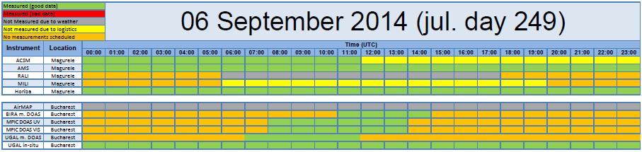
43 Page 42 of 134

44 Table 4: Data acquisition tables presenting daily data availability during AROMAT-I. Page 43 of 134

45 5. Data analysis 5.1 NO2-sonde (KNMI) Algorithms for the NO2-sonde Fundamental to the NO2-sonde is the observation that when air is bubbled through a basic (ph 12.2), watery solution of luminol, an amount of blue light is produced that is proportional to the concentration (kg/m 3 ) of NO 2 in the air. The main challenge of the NO2-sonde is the minute amount of light that is produced. On the one hand, the atmospheric concentration of NO 2 is very low (in the order of parts-per-billion (ppbv), on the other hand, the reaction between NO 2 and luminol appears to be very inefficient. In order to get sufficient signal photodiodes are used that have a high surface area to detect the blue light. Photodiodes convert this light to an electrical current that is proportional to the amount of light received, over many orders of magnitude. This current is fed through an OPAMP that converts the current into a voltage. The photodiode + OPAMP system generates a small but temperature dependent offset. Figure 32 (left): Schematic overview of the NO2-sonde measurement principle. Figure 28 (right): Picture of the NO2-sonde inner electronics. The photodiodes were found to also produce a current when exposed to a temperature gradient, while in the NO2-sonde temperature gradients always develop during measurement. Therefore, to compensate for this effect, a second array of photodiodes is used, that is mounted behind an aluminum film. This array is referred to as the "blind" array, since its photodiodes are exposed to the same temperature gradients as the "seeing" photodiodes, but the light from the reaction cannot reach them. The seeing and the blind photodiodes will give a signal in Volt: Vs = R * l + Os + R * G Vb = Ob + R * G Page 44 of 134

46 Table 5: Calculation of the signal from the photodiodes of the NO2-sonde. Vs: voltage from the seeing photodiodes Vb: voltage from the blind photodiodes R: amplification of the current to voltage converter l: amount of light Os: offset of the seeing amplifier Ob: offset of the blind amplifier G: temperature gradient over the photodiodes Vs - Vb = R * l + ( Os - Ob ) Table 6: Calculation of the amount of light resulting from the chemical reaction between luminol and NO 2. Which is rephrased as: l = ( Vs - Vb - D ) / R Table 7: Rephrased calculation from table 6, introducing temperature dependent dark Voltage D. D: temperature dependent dark voltage Note that the dark voltage "D", can be determined by replacing the luminol solution with water. In this case "l" is zero, and D = Vs Vb. The dark voltage is normally parameterized as: D = a0 + a1 * exp ( T * a2 ) Table 8: Calulation of the 3 parameters describing the detector dependent dark voltage. Where T is the temperature in degrees Celsius. a1, a2, a3 are determined in the laboratory prior to flight, the values used in the AROMAT-I campaign, are shown in table 10. In order to get the observed amount of NO 2, we need to correct for: cp(t) = pump rate (at the ground) ce(p) = pump correction (at altitude) cs(t) = sensor efficiency P = ambient pressure divided by hpa All these corrections are formulated in such a way that they are close to 1 at standard pressure and temperature. Page 45 of 134

47 So finally: NO 2 = ( Vs - Vb - D ) * cp * ce * cs * C / P Table 9: Calulation of the concentration of NO 2 measured by the NO2-sonde cp(t) = ( T + K + 5 ) / ( K + 30) ; K = Celsius Ce(P) = 1 in the troposphere Cs(t) = exp ( ( T - 25) * 0.02 ) The final constant "C" is basically unknown, and should ideally be obtained through calibration of the NO2-sonde against a known source of NO 2, or by inter-comparing NO2-sondes. As is shown table 10, sensors were used with a wide variety of C values. date sensor Launch (m) A0 (V) A1 (V) a2 C (pppv/v) F58/T F42/T F60/T F65/T F67/T F68/T F64/T F42/T F50/T F52/T F69/T Table 10: Values for dark voltage parameters a0, a1 and a2, and for calibration constants C, as used during AROMAT-I Precision of the NO2-sonde For large signals, a measurement error of 10% or less should be achievable. There are a number of sources of errors that normally are ignored, which may introduce an error of a few percent. The most important source is a change in instrument sensitivity due to a change in ph value of the solution. Sensing solution acidification is caused by a reaction between its strong base KOH and CO 2 from ambient air. Another error is introduced by the temperature dependent flow through the pump. Ideally, the temperature inside the pump cylinder would be measured, but instead the sensor temperature plus five degrees Celsius is used as a proxy. However, the largest source of uncertainty is introduced when calibrating the sonde against a "known" source of NO 2. The method used most of the time, has been comparing the results of the NO2-sonde with another instrument in the field. Page 46 of 134

48 Figure 33 (left): 4 NO 2 -sondes measuring side-my-side commercial NO x -analyzer inlet. Figure 29 (right): Voltage recorded by each sonde scaled to NO 2 concentration in ppbv simultaneously recorded by the commercial NO x -analyzer. In our experience, this is the most significant source of uncertainty the NO2-sonde is subjected to, because of one of the following situations: - The instrument used for comparison was poorly calibrated. - During the comparison of the NO2-sonde and another instrument, the NO 2 concentration was not sufficiently high. - The instrument used for comparison was sensitive to other Nitrogen compounds (NO y ). - No instrument was available for comparison. In the last case one has to revert to a "theoretical" sensitivity of the NO2-sonde, a value that can be off by up to 50%. It is important to point out, that in case the calibration is poor, the shape of the obtained NO2- profile is not affected. Page 47 of 134

49 Figure 34: 11 NO 2 vertical profiles recorded during AROMAT-I, all flown from Turceni. For very small signals, other sources of errors become important. This is very relevant, because the NO2-sonde will normally reach altitudes where almost no NO 2 is present. Often, still a signal appears to be present. Two sources of spurious signals have been identified. 1) The NO2-sonde has a small sensitivity to ozone in the order of magnitude of 2 % per molecule. It is difficult to correct for this effect when the actual ozone profile has not been measured. 2) There could be an error introduced by the data-acquisition hardware. Ideally, the dark voltage "D", should be measured using the same data-acquisition system as is used during the flight of the sonde, thus using a radiosonde for data recording. However, D is parameterized in the lab using another type of datalogger, which could introduce an offset in the data. Efforts were made to minimize the effect, but there are practical limitations on how well this can be done. (For example: Unknown remains the fact whether the offsets in the data acquisition systems are temperature, pressure, or humidity dependent). The assumption is made that the remaining offsets could be in the order of a few millivolts, in Vs, Vb and D Parameters received from the radiosonde Details of the data processing in the radiosonde, or its ground station, have not been published. Therefore the information in this paragraph is limited to quoting the estimated accuracy of the results from various sources. (Note that the radiosondes were not calibrated before launch during the AROMAT-I campaign.) time 1 second Page 48 of 134

50 altitude 5 meters, see note below pressure 1 hpa temperature 0.2 Celsius relative humidity 5 %-points position 10 meters wind speed 0.15 m/s wind direction 10 degrees, divided by wind speed in m/s Table 11: Radiosonde parameter accuracy. Note on altitude: The altitude is computed from pressure, temperature and humidity, assuming hydrostatic equilibrium. The most important source of error, is the estimation made for the altitude (height above sea level) of each launch point. The following assumptions were made: Football field 122 meter ASL UAV field 116 meter ASL Hotel car-park 127 meter ASL Table 12: Altitude estimations for NO2-sonde launch locations. 5.2 Aerosol Particle Sizer (APS) Data processing procedure: the instrument has proprietary software processing routines to provide all data products in ASCII and graphical formats. Error calculation: since the data processing routines are not available for the end-user, the associated uncertainties are related only to systematic errors provided by the manufacturer. 5.3 SWING (BIRA-IASB) The data analysis of SWING measurements consists of three steps: (i) a DOAS analysis of the spectra (ii) the georeferencing of these slant columns, (iii) the conversion to vertical column using air mass factors DOAS analysis The first step is achieved with the QDOAS software (Danckaert et al, 2014) using the settings presented in table 13. Figure 35 shows an example of a DOAS fit of NO 2 in one of the SWING spectra recorded downwind of the Turceni power plant during AROMAT (11 September 2014). For this DOAS fit, the SNR (understood as the ratio between the slant and its error) is 24. Page 49 of 134

51 Spectral range nm NO2 Van Daele et al (98) O4 Hermans H2O Harder and Brault (97) O3 Burrows et al. (99) Ring Chance and Sputr (97) Polynomial order 5 Table 13: DOAS settings used for the analysis of the SWING spectra Figures 35 (left):doas fit of NO2 in a SWING spectra. The measured optical depth (differential and relative to a reference spectrum) appears in black while the red curve is the laboratory NO2 cross-section. It should be noted that by definition the DOAS analysis is performed with respect to a reference spectrum and that for SWING, this reference spectrum is chosen amongst the zenith measurements (SWING was set to record a zenith measurement every 500 spectra) and selected based on ancillary measurements to be above a clean area, upwind of the power plant (see Fig. 36). Figure 36: Tracks of the SWING flight in September 11 and position of the reference spectrum. Mobile DOAS measurements indicate that this reference was recorded outside the plume. Page 50 of 134

52 The outcome of the DOAS analysis are the time series of DSCDs, of which an AROMAT-1 example can be seen in Fig. 37. The UAV was performing loops and overpassing Turceni exhaust plume. The error on the DSCDs is visible on the zoom in the top of Fig. 37 and indicates a SNR of around 25 above the plume. Figure 37: Time series of NO 2 DSCDs during a SWING-UAV flight, with a zoom on one plume overpass showing also the error bars Georeferencing of the slant columns The second step of the SWING data analysis implies to assign a position to each measurement first on the UAV track and then on the ground. This step would be straightforward if the computer in SWING was recording the position and attitude together with the spectra but due to size and speed issues, the attitude information and GPS were recorded by the UAV pc instead. Figure 38 presents some examples of the GPS and attitude angles (pitch and roll) as measured by the IMU of the UAV during the flight on 11 September Page 51 of 134

53 Figure 38: Attitude and GPS measurements recorded on the UAV computer. The SWING PC clock was synchronized with the GPS time in the field before the measurements, which was useful but not accurate enough. Therefore, in a second step, we used the pressure measurements in SWING to derive a SWING altitude that was aligned with the GPS altitude of the UAV (See Figure 39). Finally, a fine alignment was done making the signal level in the spectra coherent with the angular distance to the sun. Figure 39: Time series of the altitudes recorded during the flight on 11 September 2014 by (green) the GPS of the UAV and (blue) the pressure sensor in SWING Once the spectra accurately time-referenced, the pixel projection on the ground was achieved using the UAV position, scanner position, and attitude angles using the geometric formulas in Schonardt et al. (2015). Page 52 of 134

54 5.3.3 Conversion to vertical columns The DSCD retrieved by the DOAS analysis is related to the tropospheric vertical columns (VCD t ) by the following expression DSCD = AMF t VCD t + SCD S SCD ref Where SCD s is the stratospheric slant column density, AMF t is the tropospheric air mass factor, and SCD ref the residual column in the reference spectrum. Considering that this reference spectrum was chosen in a clean area and that the flights were performed in the middle of the day and lasted less than one hour, SCD s and SCD ref cancel each other, the DSCD can be considered as the tropospheric slant column, and thus VCD t simply expressed as: VCD t = DSCD AMF t The tropospheric air mass factor relates the slant column, which depends on the light path of the measurement and is thus strongly dependent on the observation geometry and atmospheric state, to the more geophysically relevant vertical column. As for the BIRA Mobile-DOAS data analysis, the AMF for SWING were calculated with the DISORT radiative transfer model (Mayer and Kylling, 2005). However, compared to the Mobile-DOAS measurements, the SWING observations in Turceni benefited from many ancillary measurements (Mobile-DOAS, LIDAR, NO 2 sonde) that could be used to fix the different geophysical parameters in the radiative transfer model. In particular, the NO 2 profile in DISORT simulations was set as a 900 m thick box profile from the measured boundary layer height measured with the LIDAR (around 1 km altitude at the time of the flight) and from the sonde profile. The visibility was set to 15 km from the extinction (β) retrieved (2e-4 m -1 ) from the LIDAR using the Koschmieder's Law: v = 3 β Figure 40 presents the air mass factors using the aforementioned visibility and NO 2 profile and in the geometry of the SWING observations as a function of solar zenith angle and for several azimuth angles. The latter is found to have a relatively small impact on the air mass factor, at least compared with the SZA Error analysis The aforementioned equation of the tropospheric vertical column VCD t depends only on the measured DSCD and on the calculated tropospheric air mass factor AMF t. Considering that several of the key parameters for the radiative transfer model could be fixed by ancillary measurements, the uncertainty on the AMF is neglected in the error budget of VCD t and the latter is expressed as: σ VCDt = σ DSCD AMF t where σ DSCD is the error on the slant column densities which is an output of the DOAS analysis. Page 53 of 134

55 Fig. 40: Air Mass Factors as a function of solar zenith angle and relative azimuth for the SWING UAV geometry (flying at 500 m.a.g.l) and the conditions of BLH and aerosol load observed during AROMAT. Figure 41 presents the time series of NO2 vertical columns measured by the SWING-UAV observation system in Turceni on 11 September 2014, and the associated 1-σ error on the tropospheric vertical columns. Figure 41: Time series of the vertical column densities in Turceni on 11 September 2014 (upper pannel) and 1-sigma associated error (lower pannel). Page 54 of 134

56 5.4 AirMAP (IUP) During the flights, spectra of scattered sunlight from below the aircraft are recorded. The datasets are series of images from the square CCD-chip with the spectral information on the horizontal axis and spatial information on the vertical axis. In the post-processing, adjacent rows of the CCD are averaged according to the illumination by the individual light fibers. This results in time series of individual spectra for each viewing direction. The spectra are georeferenced according to the to the Cessna s AHRS (Attitude and Heading Reference System), using a nearest neighbor synchronization of the GPS timestamps. The GPS-altitude is provided as the altitude above the geoid and is corrected for altitude above ground level with a digital elevation model (DEM) (European Environment Agency 2013). Spectral calibration is performed using emission lines of a HgCd-spectrum and a high resolution solar atlas (Kurucz et al. 1984). Subsequently, the DOAS method is applied to the calibrated spectra to retrieve differential slant column densities (DSCDs). The DSCD is the number density of an absorber integrated along the light path relative to the absorber amount in the reference spectrum. The reference spectrum used in the DOAS analysis is taken from a scene of the same flight with low absorber abundances. The most important settings of the DOAS retrieval for NO 2 columns are displayed in 14. Molecule Temperature Reference O K (Serdyuchenko et al. 2014) NO K (Vandaele et al. 1998) O K (Thalman and Volkamer 2013) H 2 O 293 K (Rothman et al. 2013) Ring effect (Rozanov et al. 2014) Offset Polynomial order Fit window Constant Quadratic 425 nm 450 nm Table 14: Fitted absorption cross-sections and important settings used in the retrieval of NO 2 DSCDs Derivation of vertical column densities Starting from the DSCDs of the DOAS fit, vertical column densities, defined as the absorber concentration integrated along the vertical, are computed. The conversion of the retrieved DSCD to a vertical column density (VCD) enables a comparison of measured trace gas column densities irrespective of the viewing geometry and solar position. In the following, the conversion of DSCDs to VCDs is described Computation of Air Mass Factors The light path through the atmosphere depends on the viewing geometry under which the spectra were recorded. The AMF is usually expressed in the form of air mass factors (AMF) which are defined as the ratio of slant and vertical column densities: Page 55 of 134

57 AMF = SCD VCD = DSCD + SCD 0 VCD (1) where SCD 0 is the slant column density of the absorber in the reference spectrum. The AMF is simulated by radiative transfer models (RTM). Here the SCIATRAN RTM (Rozanov et al. 2014) is used. The following parameters are considered in the calculation of the air mass factor: NO 2 -profile flight altitude (H) ground surface reflectance (A) viewing zenith angle (VZA) relative azimuth angle (RAA) solar zenith angle (SZA) wavelength (λ) The flight altitude is the altitude of the aircraft above ground. The NO 2 -profile and the flight altitude determine the sensitivity of the measurements for NO 2, because only part of the photons received at the instrument may have passed through atmospheric layers close to the ground, see Figure 42. Figure 42: Sketch illustrating the angles and 3 possible light paths. In general, the measurement sensitivity towards the presence of an absorber decreases towards the ground, and this effect gets more pronounced for increasing flight altitude. The ground spectral surface reflectance determines the fraction of light reflected at the surface, which again depends on the wavelength. Bright surfaces will increase the relative contribution of surface reflection to the signal received at the aircraft, thereby increasing the sensitivity to absorbers located close to the surface. Areas with a high surface reflectance in the fitting window will therefore generally yield lager DSCDs for the same amount of the trace gas present below the aircraft. The viewing zenith angle is the deviation from the direct nadir observation geometry. As it increases, the light paths get longer. The viewing zenith angle changes with the viewing direction, but is also Page 56 of 134

58 altered with the aircraft s attitude. The relative azimuth angle is the difference between the solar azimuth and the viewing azimuth of the measurement. Following the SCIATRAN documentation, the relative azimuth is defined as 0 if the instrument is pointed towards the sun and 180 for the direction away from the sun. The solar zenith angle is the angle between the zenith and the center of the sun's disc. The SZA has a large influence on the length of the light path through the Earth s atmosphere. The input parameters to SCIATRAN are either measured directly or are calculated from other known parameters, see table 15. Variable Source Flight altitude GPS + correction by DEM Ground surface reflectance Constant Viewing Zenith Angle (VZA) Calculated (depends on viewing direction and aircraft attitude) Relative Azimuth Angle (RAA) Calculated (from viewing azimuth angle and solar azimuth angle) Solar Zenith Angle (SZA) Calculated (from time and GPS location) wavelength Center of fitting window NO 2 -Profile Box-profile in lowest 500 m Aerosols Not considered Table 15: Input parameters for the calculation of air mass factors and their sources The unknown parameters are the surface reflectance, the NO 2 -profile and the aerosol load and profile for which approximations have to be estimated. In the current approach we assume a simple box profile of NO 2, with a homogeneous mixing ratio within the lowest 500 m. This assumption may hold true for the measurements above Bucharest where the major NO x emissions arise from traffic. The profile assumption is not likely for the emissions of the power plant in Turceni because the exhaust stacks will inject the NO x emissions in higher altitudes. The influence of the profile assumptions on the AMF are discussed in section While there are several surface reflectance products available from satellite observations (MODIS, OMLER), their spatial resolution is much too coarse for the application in our measurements. In the current version of the data product, the surface reflectance is thus set to a constant surface reflectance of The effects of this assumption are discussed in 0. This assumption on the surface albedo will be improved in a future data product by using the intensity variations observed in the measurements in combination with modelled intensities. Aerosol effects are not yet considered in the current RTM calculations for the AMF. This assumption is of course not correct. Measurements during AROMAT have shown that significant (and variable) amounts of aerosols were present during the measurements. Therefore, the next version of the data product will contain explicit assumptions on aerosol profile and optical properties. Here we will only discuss the uncertainties introduced by the current approach (see section ). Page 57 of 134

59 AMFs were computed for a large variety of the input parameters and compiled into a lookup table (LUT). The LUT is queried for each measurement and returns a linearly interpolated AMF for the conditions of the actual measurement Correction of the absorber amount in the background While satellite platforms have the advantage to be able to measure a solar spectrum without atmospheric absorption as a reference spectrum for the DOAS analysis, this is not the case for platforms operated within the Earth s atmosphere. AirMAP has in addition no option to point into the zenith direction. Thus the reference spectrum is taken in a rural scene with low NO 2 concentrations. All fitted absorber column densities are then offset by the absorber amount in the reference spectrum (SCD 0 ). This applies to both, tropospheric and stratospheric absorbers. Both parts have to be corrected in order to compute the absolute column amount. The correction for NO 2 contained in the reference spectrum can be performed using the following equations; all variables are explained in the table below: VCD = SCD AMF (2) VCD = DSCD + SC 0 AMF (3) VCD trop = VCD VCD strat (4) VCD trop = DSCD + SC 0 SC strat AMF trop (5) VCD trop = DSCD + AMF trop ref VCD trop ref + SC strat ref SC strat AMF trop (6) Table 16: Equations for the correction for NO 2 contained in the reference spectrum. In these equations, the superscripts trop and strat refer to tropospheric and stratospheric parameters, respectively. The subscript ref refers to conditions of the reference spectrum measurement. The DSCD and the AMF trop are the trace gas result and the AMF of the current spectrum. VCD : Vertical column density Page 58 of 134

60 DSCD : Differential slant column density SC 0 : Total slant column density contained in the background AMF : Air mass factor VCD trop : Vertical column density of the troposphere VCD strat : Vertical column density of the stratosphere SC strat : Slant column density of the stratosphere AMF trop : Tropospheric air mass factor trop AMF ref : Tropospheric air mass factor during conditions of the reference spectrum measurement trop VCD ref : Tropospheric VCD in the reference spectrum strat SC ref : Slant column density of the stratosphere during the conditions of the reference spectrum Equation (6) accounts for changes in stratospheric absorber slant column densities during the time of the flight. Although this would be the right way to derive the tropospheric VCD of NO 2, the stratospheric correction is not yet implemented in the current data product. Instead the VCDs are derived, setting SC strat ref = SC strat. As the duration of the AROMAT flights was relatively short, both the diurnal variation in stratospheric NO 2 column and in stratospheric AMF are not large and the impact of this simplification is therefore small (see section ). For our measurements we assume a constant value of 1x10 15 molec cm -2 for the background NO 2 VCD. This value was also used by (Popp et al. 2012) and is in the range of previously reported rural/background tropospheric columns for eastern European summer conditions from model intercomparisons and OMI data (Huijnen et al. 2010). The impact of this assumption on the uncertainties will be discussed in Results In the following, the results of the golden days are presented. The results show the VCD of NO 2 retrieved from 35 individual viewing directions in the visible spectral range. All data shown here are bin averaged VCD values on a regular grid with a spatial resolution of x The maps were then overlaid on Google Earth imagery ( The data provided on the file server contain the original georeferenced measurements in full resolution. Individual measurements with an RMS larger than 0.02 were filtered out prior to the gridding procedure. The measurements reveal strong spatial gradients and variability of the NO 2 field above Bucharest in a high spatial resolution of 60 m x 80 m. Point sources, like industrial areas, in the urban area of Bucharest can be identified. The areas covered during a research flight correspond to approx. one Page 59 of 134

61 OMI pixel (13 km x 24 km). Averaging over all of AirMAP s measurements can thus be used for satellite data validation. AirMAPs measurements can also be used to assess the signals seen by the upcoming TROPOMI measurements with a spatial resolution of 3.5 km x 7 km. The observed values of tropospheric VCDs range from background amounts up to values around 3x10 16 molec cm -2. The data shows a strong variability between 2 consecutive days (Monday / Tuesday), see section and respectively Measurements on On (Tuesday) measurements were performed in a circular flight pattern around the city of Bucharest. The flight altitude was only around 300 m. This is not optimal for the AirMAP s measurements, but restrictions on the airspace did not allow overpassing the city center or climbing to higher altitudes. Profiles dedicated to the FUBISS-ASA instrument were flown west of Bucharest, see Figure 43. Values observed on this day are generally lower, compared to the other days. This can be explained by the low flight altitude, because part of the NO 2 amount is above the aircraft and cannot be seen by AirMAP. Figure shows a zoom-in in a different color scale for better visibility. Figure 43: NO 2 vertical column densities around Bucharest measured by AirMAP on (Tuesday). Flights were performed in low altitude due to limitations of the flight permits. A constant albedo of 0.05 was assumed in the the derivation of VCDs. Measurements with an RMS larger than 0.02 were excluded. Page 60 of 134

62 Figure 44: NO 2 vertical column densities around Bucharest measured by AirMAP on (Tuesday). Zoom-in of the data shown in Figure 39. Note the changed color scale for better visibility. Flights were performed in low altitude due to limitations of the flight permit. A constant albedo of 0.05 was assumed in the the derivation of VCDs. Measurements with an RMS larger than 0.02 were excluded Measurements on On (Tuesday) AirMAP was operated in a flight pattern similar to the flight on Adjacent flight legs were flown in East-West direction starting in the South of Bucharest in an altitude of around 3.2 km, covering an area of 30 km x 18 km. Due to technical problems with the aircraft, the measurements were cut short towards the end of the research flight. Page 61 of 134

63 Figure 45: NO 2 vertical column densities above Bucharest measured by AirMAP on (Tuesday), covering an area of 30 km x 18 km. A constant albedo of 0.05 was assumed in the the derivation of VCDs. Measurements with an RMS larger than 0.02 were excluded. Slightly negative values in the North-East occur due to instrumental noise and VCD close to the detetection limit. Measurements were cut short due to technical problems of the aircraft Error analysis The total uncertainty on the vertical column originates from (i) uncertainties on the DSCDs (ii) uncertainties in the AMFs and (iii) uncertainties in the reference column. The contribution of the different uncertainties of the measurements is discussed in the following SCD error Several effects contribute to the SCD error: Shot noise from the radiance, electronic noise from the instrument, uncertainties from the cross-sections (typically around 2-3%), and errors from spectral interferences in the DOAS retrieval. The resulting individual relative fitting errors of NO 2 above the polluted city center of Bucharest range from 5% to 10%. For smaller NO 2 abundances, the relative error would become much larger as some of the error sources are absolute errors that do not scale with the NO 2 signal. Therefore a relative as well as an absolute error amounts needs to be stated. The random error of the DSCDs can also be estimated from the noise of the retrieved DSCDs in the time / region where the reference spectrum was taken, assuming that the tropospheric NO 2 column in that area is small and constant. The observations are scattered around zero, and the RMSE (rootmean-squared error) provides an estimate on the magnitude of the random errors. Due to the variation in spectral resolution, the RMSE of the DSCDs varies with the viewing direction, and ranges from 2.1x10 15 molec cm -2 in the central viewing directions to 2.7x10 15 molec cm -2 in the outer viewing directions. Page 62 of 134

64 AMF error The AMF converts the DSCDs to VCDs. Thus uncertainties on the AMF will affect the uncertainties on the VCDs directly, mainly in the form of relative errors. The largest uncertainties contributing to the error on the AMF are the unknown surface albedo and the unknown NO 2 profile, followed by aerosol effects Albedo error Figure 46 shows the dependence of the AMF on the albedo of the surface for a typical observation scenario. It can be seen, that the AMF has a strong non-linear dependence on the surface reflectance. In the urban environment, varying surface reflectance in the range of 0.03 to 0.15 can be expected, as was shown by (Popp et al. 2012) for measurements above the city of Zurich. Assuming a constant surface reflectance of 0.05 will result in an uncertainty of ±25% on the AMF for the displayed scenario. Figure 46: Dependence of the AMF on the ground albedo for a typical scenario during AROMAT for AirMAP's central viewing direction Profile Figure 47 shows altitude dependent Box Air Mass Factors (BAMF) for a flight altitude of 3.2 km, a constant surface reflectance of 5% and a solar zenith angle of 40. The BAMF represents the sensitivity of the retrieved slant column to the presence of a certain amount of an absorber like NO 2 Page 63 of 134

65 in a given altitude. Absorbers which are present closely below the aircraft altitude will have the largest contribution to the measured signal, while the relative contribution of an absorber to the measured signal decreases for absorbers close to the surface. From the figure the influence of the absorber profile on the AMF can be estimated. For the displayed scenario, a flight altitude of 3.2 km and a well-mixed box profile of 1 km height the resulting AMF would be 1.9. If the maximum profile height is reduced to 500 m, the resulting AMF would be 1.7. Under the assumption, that the profile altitude is in the range of 500m m the uncertainty of the profile on the AMF is on the order of 12%. The magnitude of the uncertainty introduced in the AMF by the profile uncertainty increases with decreasing albedo and with increasing SZA and can be of the order of 20% at lower sun. If the absorber is in an elevated layer, as one would expect for a power plant plume, the AMF is larger and less dependent on surface reflectance. Figure 47: Box Air Mass Factor in dependence of the flight altitude. The BAMF determines the sensitivity of the measurement towards absorbers in discrete atmospheric layers. The blue boxes mark the assumed profiles as discussed in the text Aerosols In the current retrieval, aerosol effects are not yet treated. Aerosols can have several impacts on the retrieved vertical columns. If a layer of aerosols is present above a trace gas it obscures the view on Page 64 of 134

66 the trace gas layer by shielding it through the increased scattering probability. This effect would bias the VCD low. On the other hand, aerosols can lead to multiple scattering effects which extend the light path within the aerosol layer. If the aerosols and the trace gas are present in the same layer, this will lead to a larger absorption of the trace gas of interest, biasing the VCD high. These considerations assume aerosols with large single scattering albedo (SSA). For absorbing aerosols, the light path enhancement effect is reduced and VCDs are low biased also in case of a well-mixed trace gas and aerosol layer. Studies for satellite observation (Leitão et al. 2010) report on sensitivities varying between a few percent and up to 20% for aerosol layers located above the trace gas of interest. The quantitative effect on the AirMAP retrieval has not been investigated yet, but this will be done for an updated data version. It is planned to constrain the assumptions on aerosol load and profile by data measured by other partners during AROMAT Error on the reference column As no direct measurements of the NO 2 column in the background scene exists, this value is quite uncertain in relative terms. Assuming a 100% uncertainty on the 1x10 15 molec cm -2 value and a tropospheric AMF of 2, this adds an uncertainty of 5x10 14 molec cm Error from missing treatment of variation in stratospheric contribution During the measurements, the stratospheric NO 2 column will change due to the diurnal photochemistry. A rough estimate would be that the NO 2 column increases by 5% per hour. In addition, the stratospheric AMF changes with SZA, in first approximation following the sec(sza). A conservative estimate would lead to a change of AMF by 0.7 between 40 and 60 SZA. Considering a typical vertical stratospheric NO 2 column of 5x10 15 molec cm -2 and a tropospheric AMF of 2, the combined error introduced by ignoring the change in stratospheric contribution is of the order of 2x10 15 molec cm Mobile-DOAS (BIRA-IASB) The data analysis of the BIRA mobile DOAS observations consists of two steps: (i) the DOAS analysis which extracts the slant columns from the fitted absorptions in the spectra and (ii) the conversion of these slant columns to vertical columns, which corrects the slant column for its light path. The first step is achieved with the QDOAS software (Danckaert et al, 2014) using the settings presented in table 17 It leads to georeferenced time series of differential slant column densities for the two channels, zenith and off-axis: DSCD zen and DSCD off. Page 65 of 134

67 Spectral range nm NO2 Van Daele et al (98) O4 Hermans H2O Harder and Brault (97) O3 Burrows et al. (99) Ring Chance and Sputr (97) Polynomial order 3 Table 17: DOAS settings used for the analysis of BIRA Mobile-DOAS spectra. The second step is achieved in two different ways for the two different sites of the campaign. We first introduce the algorithm used for the Bucharest measurements and then the one used in the Jiu Valley. 1) In Bucharest, we use the methodology described in Merlaud (2013). It assumes that, on average, the two channels (zenith and off-axis) will sample the same air masses. By using reference spectra recorded in the same conditions for both channels, and under the realistic assumption that the stratospheric slant columns are the same for the two channels, the stratospheric contributions and the reference columns cancel each other and we can express the tropospheric column as: VCD tropo = DSCD off DSCD zen AMF off AMF zen where AMF off and AMF zen are the tropospheric air mass factors in the two directions. For the BIRA Mobile DOAS analysis, these AMFs are calculated using Disort (Mayer and Kylling, 2005). The AMF represents the light path of the measurement and obviously, several of the geophysical parameters influencing the light path cannot be known everywhere for mobile doas measurements. Our way to deal with this limited knowledge consists in calculating AMF for a variety of conditions (boundary layer height, visibility, albedo, sun positions), which are then gathered in a Look up table of AMFs distributions in the 2 dimensions of the solar position: solar zenith angle (sza) and relative azimuth (relaz). In practice, the AMFs used in the retrieval will be the average of a distribution for a given (sza, relaz) and the error on the AMF will be estimated as the standard deviation of the AMF distribution (see Figure 48 for some examples of AMF Page 66 of 134

68 distribution). Figure 48: Distributions of the tropospheric AMFs used for the BIRA Mobile DOAS retrieval for four different sun position Finally, the problem of the (possible) different NO 2 field for the two channels is solved by splitting 0 the VCD tropo in two components: a smoothed part (VCD tropo ) and the remaining structured ) part: (VCD tropo 0 VCD tropo = VCD tropo + VCD tropo The filtering is achieved with a sliding average of n (100) points. 0 = DSCD off DSCD zen AMF off AMF zen VCD tropo n The structured part of the vertical column is expressed only with DSCD zen, wich is less affected by obstructions: VCD tropo = DSCD zen DSCD zen n AMF zen Page 67 of 134

69 The error analysis of the two aforementioned equations leads to: σ VCDtropo 0 = VCD 0 tropo AMF σ AMF 0 From the look up table described above, this error is assumed to be constant and 10% of VCD tropo. σ VCD tropo = σ 2 DSCDzen AMF zen 2 + VCDtropo 2 AMF zen 2 σ2 AMF zen These error components are summed in quadrature, which yields the total error on the vertical tropospheric error. Figure 49 shows the retrieved tropospheric NO 2 VCDs for the measurements performed on 5 September 2015 in Bucharest. Figure 49: BIRA tropospheric NO2 column by mobile-doas measurements performed on 5 September 2014 (Bucharest) 2) In the Jiu Valley, the retrieval method presented above appeared to be difficult to apply since the NO2 field is so heterogeneous due to the strong point sources of the power plants that even on average, the air masses are two different for the two channels. To illustrate that, let us consider the case of the car driving close and toward an exhaust plume and Page 68 of 134

70 turning before driving under it. The off-axis channel could see a very strong plume but nothing at all would be detected in the zenith direction. Such an effect is (to a less dramatic extent) visible on the DSCD time series shown on Fig. 50 e.g. around 15h30 UT (the car was arriving in Turceni). Figure 50: Time series of NO2 and O4 DSCDs measured on 7 September The three peaks respectively correspond to the power plants of Craiova II, Isalnita and Turceni. We have thus used another method for the vertical column in the Jiu Valley, which uses only the zenith channel. This method is presented in Constantin et al. (2013), and is also used to analyze the Uni. Galati Mobile DOAS measurements during AROMAT, and thus detailed in the following Section (5.6). Note however that the BIRA Mobile-DOAS measurements were analyzed using the zenith air mass factors described above for the two channels algorithms, and are not the same as the AMFs used for the measurements of Uni. Galati. Page 69 of 134

71 Figure 51 Zenith Air Mass factor used for the analysis of the BIRA mobile DOAS measurements in the Jiu Valley Fig 52 shows a color map of the NO2 DSCDs measured on 11 September 2014 in Turceni between 6h30 and 14 UT (red corresponds to elevated columns). Figure 52 BIRA Mobile DOAS NO2 measurements on 11 Sept 2014 (golden day in Turceni) see below for vertical columns Page 70 of 134

72 These DSCDs were converted in vertical columns as described above and their time series are shown below in Fig 53. The maps corresponding to these measurements can be seen in section 8 (Turceni case study). Figure 53: NO2 tropospheric VCD on 11 September 2014 (golden day in Turceni) Figure 54 presents two example of measurements with the BIRA Mobile DOAS instrument in Bucharest (5 September 2014) and in the Jiu Valley (7 September 2014). Figure 54: NO2 tropospheric vertical column maps from the BIRA Mobile-DOAS from September 5 th (left) and September 7 th (right). Page 71 of 134

73 5.6 Mobile-DOAS (UGAL) The analysis of the zenith-sky spectra recorded during AROMAT-2014 was performed using the QDOAS 2.0 software, a program dedicated to the DOAS retrieval of atmospheric trace gases from ground-based and satellite measurements. The analysis is focused only on NO 2 and SO NITROGEN DIOXIDE (NO 2) Spectral analysis Table 17 presents the settings used on QDOAS to retrieve the NO 2 DSCDs. The DOAS NO 2 analysis was performed using a reference spectrum with a low NO 2 content, this spectrum was recorded on 02 September 2014 at 9:00:00 at the periphery of Bucuresti city. This spectrum was selected to represent and to determine the NO 2 amount in the reference spectrum. An example of NO 2 spectral fitting by QDOAS is represented in Figure 55. NO 2 NITROGEN DIOXIDE Wavelength range Gaps nm none Polynomial degree 5 Intensity offset Ring spectrum Trace gas cross sections constant NDSC Ring no2_298k_vandaele.xs no2_220k_vandaele.xs Table 17 NO 2 DOAS analysis settings o3_223k_bogumil.xs Ring_NDSC2003.xs H2O_HITEMP_2010_ _296K_1013mbar_air.txt O4_thalman_volkamer_293k_air.txt Page 72 of 134

74 Figure 55. The NO 2 spectral fitting of spec. no. 350, recorded on 10 sept 2014 around Turceni VCD conversion Tropospheric NO 2 VCD retrieval is based on the algorithm presented by Constantin et al., This method presents three steps. First the NO 2 amount in the reference spectrum is determined from ground-based measurements performed at twilight-sunset, using a photo-chemically modified Langley plot (Figure 56). The second step consists in determining the stratospheric NO 2 SCD content by means of the assimilated vertical stratospheric column from the satellite DOMINO NO 2 product (Table 18). To determine the diurnal variation of stratospheric NO 2, PSCBOX model simulations were used. Finally, the tropospheric VCD was determined using a tropospheric AMF calculated with the RTM UVspec/DISORT. The NO 2 profile used for AMF calculations for Turceni DOAS observations is based on the KNMI NO 2 sonde measurements. For Bucuresti, the AMF calculations are based on an NO 2 profile retrieved from CHIMERE model having as source Timisoara city. An example of tropospheric NO 2 VCD retrieval is presented in Figure 57. Below are introduced the equations used for the tropospheric NO 2 retrieval: SCD AMF (1) VCD The total slant column density in a measured spectrum (SCD meas ) is defined by Eq.2: SCD DSCD (2) meas SCD ref where the Fraunhofer reference spectrum or SCD reference (SCD ref ) is unknown. Page 73 of 134

75 Stratospheric and tropospheric content of NO 2 contribute to the measured slant column density, according to: AMF tropo VCD AMF VCD DSCD SCD (3) tropo strato strato ref Thus the VCD of NO 2 in the troposphere is given by VCD tropo DSCDmeas SCDref AMFstrato VCD strato (4) AMF tropo where AMF strato and AMF tropo are the stratospheric and tropospheric AMFs respectively. The VCDstrato used for retrievals was extracted from OMI (DOMINO) v2.0 (Table 18). The NO 2 amount in the reference spectrum was obtained from ground-based zenith-sky observations at sunrise on 21 July The measurements performed on 21 July 2014 were recorded in a rural area close to Galati city. Figure 56 represents the Langley-plot, as was mentioned above the Langley-plot is based on spectra recorded out of campaign but analyzed with a reference spectra recorded during AROMAT-1 in Bucuresti. Figure 56. The Langley-plot for SZA of measurements on 21 July 2014 with respect to a reference spectrum measured on 02 September 2014 (9:00:00 UTC), in Bucuresti city Page 74 of 134

76 Day Orbite Nr. Overpass time UTC Strato VCD [molec./cm 2 ] Pixel center( ) 1 September :54: e / September :59: e / September :41: e / September :47: e / September :29: e / September :12: e / September :17: e / September :00: e / September :43: e / September :48: e / September :53: e / September :35: e / September :41: e /44.59 Table 18. Information on the OMI (DOMINO) data used for Bucuresti/Turceni NO 2 retrievals. Figure 57. The NO 2 DSCD and tropospheric VCD from the spectra recorded around Turceni on 10 September Page 75 of 134

77 Tropospheric AMF simulations The AMFs simulations presented in this report were performed using the radiative transfer model (RTM) UVspec/DISORT. For the tropospheric AMF simulations over Bucuresti was used an NO 2 profile from Timisoara (Romania) obtained from the CHIMERE model. For Turceni observations was used a profile recorded in Turceni by the KNMI NO 2 sonde. The AMFtropo simulations were made by setting a grid of 10 km altitude and the wavelength for NO 2 simulations at 440 nm. Also was set an albedo of 0.1 and a vibility of 10km Error analysis Each parameter used in the determination of tropospheric VCD has a contribution to the accuracy of the final retrieval. The error propagation on tropospheric VCD (σvcd) can be expressed by Equation (5): σ VCD 2 tropo σ DSCD AMF tropo 2 σ SCD ref AMF tropo 2 σ SCD strato AMF tropo 2 SCD tropo AMF2 tropo σ AMF tropo 2 (5) Each error is explained below: - the error on the DOAS fitting (σ DSCD ) is determined by QDOAS. This error is generally less than 1x10 15 molec./cm 2. - the error on the estimation of the slant column in the reference spectra (σ SCDref ) was obtained by running the Langley plot for SZA=90-80, σscdref=5.681x10 14 molec./cm 2. - the error on the stratospheric SCD (σ SCDstrato ) is the uncertainty on the assimilated stratospheric slant column from DOMINO data product v2.0. This error is based on observation-forecast statistics and is estimated to be molec./cm2. - the error from the AMF simulations (σ AMFtropo ) is the error resulted from AMF simulations.the AMFtropo uncertainties are estimated at 10% 20%, for SZA increasing from 20 to 85. The typical error on the retrieved NO 2 tropospheric VCD generally is less than 25% SULPHUR DIOXIDE (SO 2) Spectral analysis For the analysis of the SO 2 DSCD was selected a spectrum with a very low SO 2 content. Due to the very low SO 2 amount in the SCD ref the DSCD is considered as SCD. DSCD was neglected when the tropospheric SO 2 VCD was calculated. Table 19 introduces the DOAS settings and cross-section used for the SO 2 retrieval from the spectra recorded during AROMAT-1. An example of SO 2 spectral fitting is represented in Figure 58. Page 76 of 134

78 SO 2 SULFUR DIOXIDE Wavelength range Gaps nm none Polynomial degree 5 Intensity offset Ring spectrum Trace gas cross sections constant yes o3_223k_bogumil.xs so2_294k_vandaele. Table 19. SO 2 DOAS analysis settings. Ring conv. o3a_243k_bogumil.xs Figure 58. SO 2 spectral fitting of spec. no. 350, recorded on 10 sept 2014 around Turceni VCD conversion SO 2 VCD retrieval is based on the conversion of the DSCD to VCD by applying the tropospheric AMF calculated for tropospheric NO 2 retrievals. In Figure 59 is represented the SCD (DSCD) and calculated VCD determined around Turceni on 10 September Page 77 of 134

79 Figure 59. The SO2 SCD and calculated VCD observed around Turceni on 10 September Selected results In this section some of the most interesting results are introduced. Figure 60. The map of tropospheric NO2 VCD recorded on the Jiu Valley on 10 September A very high amount of NO2 is observed close to the power plants located in Craiova, Isalnita and Turceni.. Page 78 of 134

80 Figure 61. The map of tropospheric NO2 VCD recorded on Bucuresti city on 2 September Figure 62. Figure 8. The map of SO2 DSCD recorded on the Jiu Valley on 10 September A very high amount of SO2 is observed close to the power plants located in Craiova, Isalnita and Turceni. Page 79 of 134

81 5.7 Mobile-DOAS (MIPC) The data analyses contains two basic steps (spectral retrieval and conversion to tropospheric VCDs), which are described in detail in the next sections Spectral Analysis The target species analyzed so far are NO 2, SO 2, and HCHO. The properties of the different analyses are summarized in Table 20. It should be noted that: a) NO 2 was analyzed from both instruments, and very good agreement between both analyses was found (see Fig. 63). Because of the much better spectral resolution, the NO 2 standard product (submitted to the file server) was analyzed using spectra from the UV instrument. b) HCHO was analyzed from spectra of the UV instrument only on an experimental basis. On several days, enhanced HCHO dscds could be detected around Bucharest (see Figs. 64 and 65). So far, results were not uploaded to the file server. c) SO 2 was only analyzed from the UV instrument. The results were uploaded to the file server. d) In principle O 4 and H 2 O can be analyzed in various spectral ranges of the spectra of the vis instruments. However, these analyses are still in an early stage, and no data were uploaded so far to the file server. NO 2 (UV) NO 2 (vis) SO 2 HCHO Wavelength range nm nm nm nm Gaps nm nm nm none none Polynomial degree Intensity offset constant constant constant constant Ring spectrum Two Ring spectra calculated from Fraunhofer reference spectrum using DOASIS Two Ring spectra calculated from Fraunhofer reference spectrum using DOASIS One Ring spectrum calculated from Fraunhofer reference spectrum using DOASIS Two Ring spectra calculated from Fraunhofer reference spectrum using DOASIS Trace gas cross sections NO 2 (Vandaele, 294K) O 3 (GOME, 241K O 4 (Greenblatt, NO 2 (Vandaele, 294K) O 3 (GOME, 241K O 4 (Greenblatt, SO 2 (SCIAMACHY, 293K) NO 2 (Vandaele, 294K) HCHO (Meller, 29K) NO 2 (Vandaele, 294K) O 3 (Bogumil, 223K, Page 80 of 134

82 NO2 DSCD AROMAT-I: Final Report Version: Final Doc-ID: AROMAT-FR-1 296K) 296K) O 3 (GOME, 241K I o correction) H 2 O (HITRAN, 290K) H 2 O (HITRAN, 290K) O 3 (Bogumil, 243K, I o correction) O 4 (Greenblatt, 296K) BrO (Wilmouth (1999), 228K) Table 20: Overview about the properties of the different spectral analyses 9E+16 2 September E+16 5E+16 Vis NO2_400_448.SlCol(NO2) nm Vis NO2_425_490.SlCol(NO2) nm UV NO2.SlCol(NO2) nm 3E+16 1E+16-1E+16 06:00 08:00 10:00 12:00 14:00 16:00 Time Fig. 63 On 2 September 2014 measurements in only zenith direction were performed. The figure presents a comparison of the retrieved NO 2 dscds from both MPIC instruments. For the visible instrument two analyses were performed: one with the same spectral range as for the UV instrument, and a second with an optimised, larger spectral range. Good agreement was found for both instruments and both spectral ranges. On this day only very low tropospheric NO 2 signals were found. The systematic increase at the end of the day represents the stratospheric NO 2 absorption (strong SZA dependence). Page 81 of 134

83 HCHO VCD [molec/cm²] HCHO VCD [molec/cm²] AROMAT-I: Final Report Version: Final Doc-ID: AROMAT-FR-1 Fig. 64 Example of a spectral analysis of HCHO (7 Septemver, 13:00). The HCHO absorption can be clearly seen in this measurement. 4E+16 5E+16 3E+16 4E+16 3E+16 2E+16 2E+16 1E+16 1E :00 7:12 8:24 9:36 10:48 12:00 13:12 14:24 7 September Time Fig. 65 Left: HCHO dscd derived from measurements at 22 elevation for a selected day (7 September). Right: HCHO dscds observed for a period of 5 days (7 September to 12 September). On 2 September NO 2 dscds measured in zenith direction were analyzed from the different groups (with the cars driving at the same route with very short distances between them). In Fig. 66 the results from the different groups are compared using the same wavelength range (which is different from our standard range, see Table 20). Except for high SZA very good agreement of all three data sets is found. Page 82 of 134

84 NO2 DSCD [molec/cm²] AROMAT-I: Final Report Version: Final Doc-ID: AROMAT-FR-1 1.6E E E+17 1E NO2_411_449.SlCol(NO2) BIRA nm NO2.SlCol(NO2) Uni Galati nm NO2.SlCol(NO2) MPIC nm 8E+16 6E+16 4E+16 2E E Time [hours] Fig. 66 Comparison of NO 2 dscds for the three different mobile DOAS instruments. The used spectral range ( nm) is different from the MPIC standard spectral range. It was used as a compromise between the spectral ranges of all three instruments. Except for large SZA very good agreement is found Conversion to VCDs The conversion of dscds to VCDs is performed differently for NO 2 and SO 2. NO 2 For NO 2, the following procedure (see also Wagner et al., 2010) is applied: In the first step, a time-dependent offset is derived from the NO 2 dscds retrieved from 90 and 22 elevation angles: DSCD offset SZA AMF trop 90 DSCDmeas AMFtrop DSCDmeas 90 AMF AMF 90 trop trop (1) Here we use the geometric approximation for the calculation of the tropospheric air mass factors (AMF). This offset is displayed in Fig. 67 (middle panel). In the next step a simple functional curve is fitted to the time-dependent offset: DSCD offset ( SZA) SCD ref VCD strat 1 cos( SZA) (2) Here the first term on the right side represents the NO 2 dscd of the Fraunhofer reference spectrum. The second term on the right side represents the stratospheric NO 2 dscd, which is expressed as Page 83 of 134

85 stratospheric NO 2 VCD times the stratospheric AMF. Here it is assumed that a) the stratospheric NO 2 VCD is constant during the measurements and b) the stratospheric AMF can be approximated by a simple geometric AMF. Both assumptions are roughly fulfilled for SZA < 80. In the last step the fitted time dependent NO 2 dscd offset is added to the NO 2 dscds derived from the measurements at 22 elevation angle, and the sum is then divided by the tropospheric AMF for 22 elevation angle: DSCD VCD 22 ( SZA) DSCD 1 sin(22 ) offset SZA (3) The resulting tropospheric NO 2 VCD is presented in Fig. 67 (bottom). Compared to other methods, our approach has two important advantages: a) Even for cases with low and homogenous tropospheric NO 2 VCDs, a realistic tropospheric NO 2 VCD can be retrieved. For measurements using only zenith observations such situations are problematic, because it will be difficult (if not impossible) to determine the NO 2 dscd of the Fraunhofer reference spectrum. b) Because of the use of a low elevation angle, the sensitivity for tropospheric NO 2 is larger that for measurements using only zenith observations. Despite of these advantages there is also an important limitation: if measurements are performed in the vicinity of localised and strong emission sources (e.g. close to power plants), the basic assumption of the method is not fulfilled: that on average observations at all elevation angles probe the same air masses. Thus in such cases, this method has to be slightly modified and applied with care. The respective modifications which are applied for SO 2 are described in detail in the next section. Page 84 of 134

86 Fig. 67 Different steps of the retrieval of NO 2 VCDs. Top: NO 2 dscds for both elevation angles (22 and 90 ). Slightly higher values are found for 22 elevation indicating the presence of tropospheric NO 2. Middle: The red curve represents the model function (equation 2) to the derived dscd offset (blue). Bottom: The resulting tropospheric NO 2 VCD derived from the measurements at 22 elevation angle (equation 3). SO 2 Because of the limitations of the approach described above for localised emission plumes (and because no significant stratospheric absorption has to be considered for SO 2 ), for the conversion from SO 2 dscds into SO 2 VCDs a slightly different method is applied: Like for NO 2 an offset function (equation 1) is calculated (Fig. 68 middle). However, now data from measurements with very high SO 2 dscds (from the power plant plume) are excluded, because they don t fulfill the requirement of horizontal homogeneity. Also for the model function (equation 2) only the first term on the right side is considered, because the stratospheric SO 2 absorption is negligible (the red line simply describes the average of the blue values). In the final step the offset value is added to the measured dscds at 22 elevation and the SO 2 VCDs are calculated using the geometric approximation (equation 3). Despite these modifications it should be noted that the derived SO 2 VCDs of the power plant plumes have to be still interpreted with care: in some of these cases, even the SO 2 dscds might be the better suited quantity for the geophysical interpretation of the measurement results, i.e. the SO 2 dscd might better represent the integrated SO 2 concentration across the diameter of the observed plume. Page 85 of 134

87 Fig. 68 Different steps of the retrieval of SO 2 VCDs. Top: The NO 2 dscds for both elevation angles (22 and 90 ). Very high value are found for particular periods of the measurements related to the emission plume of the power plant. Middle: The dscd offest calculated from equation 2. However, measurements strongly affected by the power plant emissions are excluded. The red curve represents the average of the derived dscdoffset. Bottom: The resulting tropospheric SO2 VCD derived from the measurements at 22 elevation angle (equation 3) Selected Results In this section some of the most interesting/important results are presented. Fig. 69 presents an overview of all SO 2 for the whole campaign. Strongly enhanced values are found in the second week, caused by the power plant emissions. Fig. 70 shows simultaneous results for NO 2 and SO 2 for measurements close to the power plants. Fig. 71 shows a comparison of the spatial patterns of NO 2 and SO 2 close to the power plant for 10 September. Fig. 72 shows a comparison of the spatial patterns of NO 2 and SO 2 around Bucharest. Although the SO 2 analysis is close to the detection limit, similar spatial patterns of both species are found. Page 86 of 134

88 SO 2 SCD [molec/cm²] NO 2 SCD [molec/cm²] SO 2 SCD [molec/cm²] NO 2 SCD [molec/cm²] AROMAT-I: Final Report Version: Final Doc-ID: AROMAT-FR-1 Figure 69: SO 2 SCDs observed during the whole campaign. In the first week (around Bucharest) rather low values are found. In the second week (close to Turceni) strongly enhanced values are observed (only measurements for SZA < 75 and RMS < 2%). 1.8E+18 SO2_SCD_corr NO2_corr 1.8E E E+18 SO2_SCD_corr NO2_corr 4.8E E E E E E+17 8E+17 8E E E+17 3E+17 3E+16 8E+17 8E+16-2E+17-2E+16 4:48 7:12 9:36 12:00 14:24 16:48 19:12 10 September -2E+17-2E+16 4:48 7:12 9:36 12:00 14:24 16:48 19:12 11 September Fig. 70 Comparison of dscds of NO 2 and SO 2 close to the power plant of Turceni. The similarity of the indicates a common emission source. Page 87 of 134

89 Fig. 71 Comparison of NO 2 VCDs and SO 2 SCDs around Turceni for 10 September Strongly enhanced SO 2 SCDs (note the colour scale) are observed close to the power plant. Fig. 72 Comparison of NO 2 VCDs and SO 2 SCDs around Bucharest for 5 September Although the SO 2 dscds are close to the detection limit, enhanced values of both species are found at similar locations in the west of Bucharest. Page 88 of 134

90 5.8 Multiwavelength Raman LIDAR (RALI) Data processing procedure Backscatter coefficient: Fernald-Klett algorithm with constant LIDAR ratio (assumed) (Klett, 1978) Extinction coefficient: calculation of the column-averaged LIDAR ratio by constraining the integrated extinction to the co-located sun photometer AOD; the backscatter profile was extrapolated to the ground based on a polynomial fit of the profile PBL height: altitude of the maximum negative gradient of the range corrected signal at 1064nm channel (Belegante et al., 2013) Error calculation Propagation of the statistical error through the calculus chain. Assumption of 10-15sr uncertainty for the LIDAR ratio, depending on the temporal differences between LIDAR and sun photometer measurements. 5.9 UV scanning LIDAR (MILI) Data processing procedure Backscatter coefficient: Fernald-Klett algorithm with constant LIDAR ratio (assumed) Extinction coefficient: calculation of the column-averaged LIDAR ratio by constraining the integrated extinction to the AOD estimated from MODIS; MODIS AOD was calculated at 500nm and converted to 355 nm using the Angstrom exponent retrieved from the sun photometer measurements at Bucharest and Cluj (mean value); the backscatter profile was extrapolated to the ground based on a polynomial fit of the profile PBL height: altitude of the maximum negative gradient of the range corrected signal Error calculation propagation of the statistical error through the calculus chain assumption of 10-15sr uncertainty for the LIDAR ratio, depending on the temporal differences between LIDAR and sun photometer measurements Page 89 of 134

91 5.10 Aerosol Chemical Speciation Monitor (ACSM) Data processing procedure: Diagnosis of several parameters: vaporizer, filter, air beam, chamber temperature Data corrections using relative ionization efficiencies and the collection efficiencies Econvolve the raw ACSM mass spectra into chemically speciated mass spectra Application of conversion factors to translate ion signal to µg/m 3. Error calculation: Not Applicable 5.11 C-ToF Aerosol Mass Spectrometer (AMS) All processing procedures are available at The basic steps in processing the AMS data are: Check calibrations: m/z, baseline, single ion Do corrections: air beam, flow rate, time of flight Recalculation of raw spectra to sticks and sticks to speciated aerosol loadings Application of conversion factors to translate ion signal to µg/m 3. Several fractions can be calculated as ratio of specific organic aerosol mass spectrum signal and total organics: f43, f44, f60. The degree of aerosol oxidations is based on f44 and f43 parameters, while f60 gives the potential to have biomass burning aerosols (Cubison et al., 2011). Error calculation: Not Applicable 5.12 Gas analysers from INOE Data processing procedure: For each component measured, the system provides four types of data: momentary values, integrated values, moving averages, and simple average. The 3 min data is used to calculate the hourly average of gas concentration (Stefan et al., 2013). Error calculation: The standard deviation of the hourly average (provided from the 3 minutes time period) is added to the instrument's linearity and span drift specs values to provide a complete systematic and statistical error analysis Gas analysers from UGAL The in-situ observations (NO, NO 2, SO 2 ) performed by the instruments onboard of UGAL s mobile laboratory are of uncertain quality. During the campaign there were many problems with the instrumental calibration and power source. As a conclusion the mobile laboratory need capital repairs. Page 90 of 134

92 Figure 73: Unrealistic NO 2 measurements outside of Bucuresti at INOE site, on 02 September Sun Photometer AERONET level 2.0 data Optical depth is calculated from spectral extinction of direct beam radiation at each wavelength based on the Beer-Bouguer Law. Error calculation: Not Applicable 5.15 Aureole and Sun Photometer 2 Main data product for FUBISS-ASA2: aerosol optical depth (AOD, NetCDF), spectral channels 412nm, 450nm, 500nm, 609nm, 778nm, 862nm. Data Analysis Fubiss-ASA2: radiation which enters the earth s atmosphere is attenuated due to absorption and scattering. The fundamental law is the Beer-Lambert law, which is strictly valid only for monochromatic irradiance, but may also be applied for channels with a small bandwidth. The aerosol optical depth τa is derived by rearranging the Beer-Lambert law: T(λ)=V(λ)/(V_0 (λ) (d_site^2) (d_cal^2 ))=e^(-m(θ)τ(λ) ) with τ(λ)=τ_r (λ)+τ_a (λ)+τ_g τ(λ)=τ_r (λ)+τ_a (λ)+τ_no2 (λ)+τ_o3 (λ) τ_a (λ)=(ln(v_0 (λ)d)-ln(v(λ)))/m(θ) -τ_r (λ)-τ_no2 (λ)-τ_o3 (λ) Page 91 of 134

93 τa τr τg τno2 τo3 : Aerosol optical depth : Raleigh optical depth : Gas optical depth (NO2, O3, CO2, H2O, for this case we neglected some gases) : NO2 optical depth : O3 optical depth V0 : calibration coefficient (calculated solar irradiance at the top of the atmosphere measured by the instrument determined by the Langley plot method) V m Θ : measurement value : relative air mass : solar elevation angle λ : wavelength (defined channels of this analysis: 412.0, 450.0, 500.0, 550.0, 609.0, 778.0, 862.0) Reference: Zieger P., Ruhtz T., Preusker R., and Fischer J., Dual-aureole and sun spectrometer system for airborne measurements of aerosol optical properties", Applied Optics, 46, Issue 35, , (2007) AROMAT-1 FUBISS-ASA2 data results: The data acquisition with FUBISS-ASA2 and the planned flight profiles were restricted by air traffic control. Only a very small number of data collection was possible far outside of the city. In addition the flight endurance and the measurement time of the other instruments would have been very limited flying a long time outside of the target area. It was planned to fly spirals in a small area during the accent and descents, but it turned out that depending of the Sun position and the movement of the Aircraft only a view times the Sun cold be followed. Therefor in most cases a data collection was not possible or only occasionally in some flight levels. It is planned to change the flight pattern with more continuously ascent and descends to improve the number of available data. Page 92 of 134

94 Data processing chain: Figure 74: Data processing chain for FUBISS-ASA2 raw data handling. Page 93 of 134

95 6. Data format 6.1 NO2-sonde, KNMI The NO2-sonde data files are ASCII files come in two different formats: The *.a files contain 1 second data, and the *.z files contain 10 second mean data. The first line of each file contains the exact time of launch (UTC). The content of the second line should be ignored. The rest of the file consists of columns that contain the following information. Column 1. Time before (negative) or after (positive) launch. Unit: seconds Precision: 1 second Missing value: N/A (if missing the whole line is removed from the file) Column 2. Altitude (=height above sea level) computed from PTU sensors. Unit: meters Precision: 5 meters. See note below. Missing value: Column 3. Ambient Pressure. Unit: hpa or mb. Precision: 1 hpa Missing value: Column 4. Ambient Temperature. Unit: Celsius Precision: 0.2 Celsius Missing value: Column 5. Ambient Relative humidity. Unit: per cent points. Precision: 5 per cent points, see note Missing value: 999 Column 6. NO2-sensor temperature Unit: Celsius Precision: 0.5 Celsius Missing value: Column 7. NO2 mixing ratio Unit: PPBV Precision: see note below Missing value: Column 8. NO2 output of seeing channel Unit: volts Precision: irrelevant Missing value: Column 9. NO2 output of blind channel Unit: volts Precision: irrelevant Missing value: Column 10. GPS longitude Unit: degrees Precision: typically 10 meters in flight, unknown at the ground Missing value: Column 11. GPS latitude Unit: degrees Precision: typically 10 meters in flight, unknown at the ground Missing value: Column 12. GPS altitude Unit: meters Precision: typically 20 meters in flight, unknown at the ground Missing value: Column 13. Number of satellites used to compute GPS products. Unit: integer Precision: N/A Missing value: 0 if GPS retrieval failed. Column 14. Wind speed Unit: m/s Precision: 0.15 m/s, see note Missing value: Column 15. Wind direction Unit: degrees from the north Precision: 10 degrees divided by the wind speed (m/s) Missing value: 999 Page 94 of 134

96 6.2 Aerosol Particle Sizer (APS) Data processing procedure: the instrument has proprietary software processing routines to provide all data products in ASCII and graphical formats. Error calculation: Since the data processing routines are not available for the end-user, the associated uncertainties are related only to systematic errors provided by the manufacturer. 6.3 SWING (BIRA-IASB) The data are provided in ascii tab-delimited files for both the DSCDs and the VCDs files.. All the files contain a header line with the field names which are generally self-explicit. 1) DSCD files: The fitted DSCDs and associated errors ( NO2.SlCol(NO2) and NO2.SlErr(NO2) ) are expressed in molec./cm 2. The position of the scanner is given by the field UAV servo sent, with 110 being nadir position. Note that the time in this file is the SWING time and must be referenced as described in the data analysis section for SWING. 2) VCD files: Contains the time and geo referenced DOAS analysis outcome. The most important parameters are the GPS and IMU information from the UAV( lat, long, alt, pitch, roll, heading ), the pixel coordinates ( longpix, latpix ) and the observation geometry ( los : line-of-sight angle to nadir, azimangle relative azimuth angle), and the vertical tropospheric columns and its associated error (respectively vc and errvc ). 6.4 AirMAP (IUP) YYMMDD[VD]II.EXTENSION YY=year MM=month DD=day [VD]=viewing direction (01 until 35) II=indicates the spectrometer used (only for internal information) EXTENSION= file name extension So for example the file with the name: II.NO2VIS contains data from , of the 4th viewing direction. The extension NO2VIS indicates that the main product of the retrieval is the column density of NO 2 in the visible spectral range. Page 94 of 134

97 The data is provided as tables in ASCII files. All files include a header that describes the data contained in the columns as well as the most important settings used in the DOAS retrieval e.g. (fit window, cross-sections etc.) 6.5 Mobile-DOAS (BIRA-IASB) The data are provided in ascii tab-delimited files and consist of three files per day of measurements: the two files for the DSCDs in the two directions and the file with the retrieved vertical columns. All the files contain a header line with the field names which are generally self-explicit. 3) DSCD files: The fitted DSCDs and associated errors ( NO2.SlCol(NO2) and NO2.SlErr(NO2) ) are expressed in molec./cm 2. Note that all the DOAS analyses were performed using reference spectra recorded on 2 September 2014 at 9 in Magurele and that we also provide plots of the time series of the DSCDs in jpeg. 4) VCD files: The most important fields are the NO2 vertical columns and its associated error (VCBira, errtot), expressed in molec./cm 2. The files also contain the air mass factors and associated errors (amf180 sig180, and amf120 sig120 for the Bucharest data). 6.6 Mobile-DOAS (UGAL) The data are in ascii format. Here is one example: for NO 2 for SO Mobile-DOAS (MIPC) The data are in ascii format. For every trace gas, there are 2 data, one for dscd and one for VCD. In every data, there are some headers, which describe the data. The VCD data has 5 parameters: longitude, latitude, time in UTC, dscd and VCD in molec/cm². The dscd data has more parameters, namely elevation angle, Total UTC-Time (number), time in UTC, SZA, longitude, latitude, RMS (root mean square), dscd in molec/cm². Here is one example: * NofHeaderlines: 11 * Instrument identifier: MPIC_Mainz_Mini Max Doas UV * Fit identifier: dscd * X-Axis = Elevation Angle ( ) * Y1-Axis = Total UTC-Time (number) * Page 95 of 134

98 Y2-Axis = UTC-Time(h) * Y3-Axis = Solar Zenith Angle ( ) * Y4-Axis = Longitude * Y5-Axis = Latitude * Y6-Axis = RMS (root mean square) * Y7-Axis = dscd (molec/cm²) [NO2, or SO2] e e Multiwavelength Raman LIDAR (RALI) The data is provided in ASCII format. All data is accompanied by data plots: quick looks files presented as time series of the Lidar backscattered profiles. The quick looks data is the temporal variation of aerosol layering for different wavelengths, providing information about the dynamics of aerosol layers in the troposphere. The maximum height of the data is given by the signal SNR. For RALI (the multi wavelength Raman Depolarization Lidar), the height of the profiles can reach 12km. For MILI (the eye-safe UV scanning Lidar), the height is depending on site conditions and Zenith angle, ranging from 0.8km to 6km. Data contains: Multiwavelength Raman Lidar - RALI\level2_0 directory SSyymmddhhmm.Ywwww SS - station name yy - year mm - month dd - day hh - hour mm - minute Y - data type: b - backscatter, e - extinction wwww - wavelength The backscatter files contain: Altitude(m) BackscatterCoefficient (1/(m*sr)) BackscatterCoefficientError (1/(m*sr)) ExtinctionCoefficient (1/(m)) - extinction from the backscatter, assuming a certain lidar ratio ExtinctionCoefficientError (1/(m)) LidarRatio(sr) - assumed lidar ratio LidarRatioError (sr) The extinction files contain: Altitude(m) BackscatterCoefficient (1/(m*sr)) BackscatterCoefficientError (1/(m*sr)) ExtinctionCoefficient (1/(m)) - measured extinction from the Raman channels ExtinctionCoefficientError (1/(m)) LidarRatio (sr) - retrieved lidar ratio from backscatter and extinction profiles LidarRatioError (sr) Page 96 of 134

99 Depolarization Lidar - RALI\Level 1_5 directory SSyymmddhhmm.Ywwww SS - station name yy - year mm - month dd - day hh hour mm - minute Y - data type: c - cross signal, p - parallel signal, d - total signal (from parallel and cross) wwww - wavelength The parallel and cross files contain: RCS (a.u.) - range corrected signal errrcs (a.u.) - errorr of the RCS RayleighFit (a.u.) - not provided AlphaMol (1/m) - not provided BetaMol (1/(m sr)) - not provided NumberDensity (1/(m^3)) - not provided The total signal files contain: RCS (a.u.) - range corrected signal errrcs (a.u.) - errorr of the RCS RayleighFit (a.u.) - not provided AlphaMol (1/m) - not provided BetaMol (1/(m sr)) - not provided NumberDensity (1/(m^3)) - not provided Depolarization Lidar - RALI\Level 2_0 directory SSyymmddhhmm.Ywwww SS - station name yy - year mm - month dd - day hh - hour mm - minute Y - data type: m - concentration data, d - depolarization data wwww - wavelength The concentration files contain: Concentration values for different aerosol components. Altitude [m] LocalCompBacksc [1/(m sr)] - local component backscatter LocalCompMass [g/m2] - local component concentration SmokeBacksc [1/(m sr)] - smoke backscatter SmokeMass [g/m2] - smoke concentration DustBacksc [1/(m sr)] - dust backscatter DustMass [g/m2] - dust concentration The depolarization files contain: Page 97 of 134

100 Altitude(m) LinearParticleDepolarization (unitless) LinearParticleDepolarizationError(1/(unitless)) 6.9 UV scanning LIDAR (MILI) Eye safe UV scanning depolarization Lidar - MILI directory SSyymmddhhmm.Ywwww SS - station name yy - year mm - month dd - day hh - hour mm - minute Y - data type: S - backscatter data, d - depolarization data wwww wavelength The depolarization files contain: Altitude (m) Volume depolarization ratio (unitlless) Volume depolarization ratio error (1/(unitless)) The backscatter files contain: Altitude (m) BackscatterCoefficient (1/(m*sr)) BackscatterCoefficientError (1/(m*sr)) 6.10 Aerosol Chemical Speciation Monitor (ACSM) All data is stored in an ASCII file format, tab delimited (or similar). All columns have explaining titles and, at the beginning of each file, the user can find a detailed header containing all information nodded for processing and understanding the data. - The data is provided in ASCII format. - The data contains: acsm_utc_time: time in UTCC Org(μg/m3): organics concentration SO4(μg/m3), NO3(μg/m3), NH4(μg/m3), and Cl(μg/m3) concentration 6.11 C-ToF Aerosol Mass Spectrometer (AMS) All data is stored in an ASCII file format, tab delimited (or similar). All columns have explaining titles and, at the beginning of each file, the user can find a detailed header containing all information nodded for processing and understanding the data. - The data is provided in ASCII format. - The data contains: acsm_utc_time: time in UTCC Page 98 of 134

101 Org(μg/m3): organics concentration, SO4(μg/m3), NO3(μg/m3), NH4(μg/m3), and Cl(μg/m3) concentration 6.12 NOx, SO2, CO, O3, THC, AND CO2 Measurements (INOE) Gas analysers data provides information of ground level concentration for several atmospheric pollutants: The concentration files contain: Time - date and time (UTC) MeasPt - not provided temp - not provided O3 - concentration (ppb) SO2 - concentration (ppb) NO - concentration (ppb) NO2 - concentration (ppb) NOx - concentration (ppb) CO - concentration (ppm) CH4 - concentration (ppm) NMHC - concentration (ppm) THC - concentration (ppm) 6.13 NO, NO2 and SO2 Measurements (UGAL) The data are in ASCII format. Here is one example: Figure 75: Example of an ASCII file containing the in-situ trace gas analyzer data from the UGAL mobile laboratory Sun Photometer In the Sun-photometer directory the following information is contained: The AOT file contains: Date(mm-dd-yy) Time(hh:mm:ss) Julian_Day AOT_1020 AOT_870 AOT_675 AOT_500 AOT_440 AOT_380 Page 99 of 134

102 7. Bucharest case study 7.1 Summary of Bucharest measured geophysical parameters Atmospheric trace gases NO 2 tropospheric vertical column: in Bucharest NO 2 tropospheric vertical columns were derived both from airborne AirMAP measurements conducted from the Cessna above the city, and from ground level measurements conducted by 3 mobile-doas systems installed on cars. NO 2 VCD trop values up to more than 3 x molecules/cm 2 were detected. SO 2 differential slant column density: was derived from one on the mobile-doas systems, the car mini MAX-DOAS system belonging to the MPIC team. Although the DSCD values retrieved were hardly above the detection limit of the instrument, the zones of elevated SO2 levels correspond to the zones of elevated NO2. NO 2 volume mixing ratio: was detected from in-situ gas analyzer measurements conducted at Magurele, although the levels detected at this site were not higher than 7 ± 5 ppb. SO 2 volume mixing ratio: was detected from in-situ gas analyzer measurements conducted at Magurele, although the levels detected at this site were not above the detection limit of 1 ppb Aerosol properties Backscatter coefficient: was derived from LIDAR measurements conducted at the INOE atmospheric observatory in Magurele both by a UV scanning LIDAR (MILI) and a Multiwavelength Raman LIDAR (RALI). Values up to 2.33 ± 0.20 and 1.30 ± /(Mm sr) were retrieved at 355 and 532 nm respectively. Extinction coefficient: was derived from LIDAR measurements conducted at the INOE atmospheric observatory in Magurele both by a UV scanning LIDAR (MILI) and a Multiwavelength Raman LIDAR (RALI). Values up to ± and ± /(Mm) were retrieved at 355 and 532 nm respectively. Planetary boundary layer height: was derived from LIDAR measurements conducted at the INOE atmospheric observatory in Magurele both by a UV scanning LIDAR (MILI) and a Multiwavelength Raman LIDAR (RALI). The retrieved height of the PBL varied between 1260±450 and 2180±800 meter during the AROMAT-I campaign. Aerosol optical depth: was measured by two sun photometers, one operated by INOE from Magurele and another one operated by FUB from Baneasa airport in the North of Bucharest, closer to the city center than Magurele. Average PM1 concentration: was derived from both C-ToF Aerosol Mass Spectrometer and Aerosol Chemical Speciation Monitor measurements conducted at Magurele, up to a level of 7.22±2.59 µg/m3. Page 100 of 134

103 Total Suspended Particles: or the mass concentration of particulate matter was derived from airborne Aerosol Particle Sizer Spectrometer measurements conducted from the INCAS UAV above the Clinceni airfield in the South-West of Bucharest, close to Magurele. Only on September 2 nd the TSP could be derived from the APS data, when it had a value of ± µg/m Analysis of the Golden Day, September 8 th Multiwavelength Raman LIDAR (RALI) Fig.76 top left: Time series Range corrected signal (RCS) at 532nm from 6 am to 6pm UTC; color gradients show different aerosols concentrations; PBL heights are represented as white crosses. Fig.77 top right: PBL heights derived from LIDAR measurements (black) varying from 300m to 2200m and PBL from ECMWF reanalysis (red) at 3am,6am,9am,12pm. Fig.78 bottom left: Backscattering vertical profiles from 800 m to 6 km, one hour averages. Fig.79 bottom right: Extinction vertical profiles from 800 m to 6 km, one hour averages From Figs. 76, 77, 78,79, it may be concluded that turbulence is dominating below 4.5 km, with successive aerosol layers at 2, 2.5 and 3.5 km. Between 7-11 AM due to high convective mixing of the air masses PBL height estimations by ECMWF is biased due to the regional scaling. During the stable phase of the PBL (after 12 PM) both methods agree on the retrieved value (~2200 m- Fig. 77). High aerosol loading is present the entire day up to Km, with the aerosol layer between 3 and 4Km decreasing during the day and mixing within the PBL. Also clouds are forming at the end of the Page 101 of 134

104 day at this level. LIDAR Ratio at 532nm in the layers is between 55 and 85 sr therefore the type of aerosol could be continental: polluted or smoke Sun photometer-time series data Fig.80 left: AOD from 08:00 to15:00 UTC. Fig.81 middle: Angstrom parameter from 08:00 to15:00 UTC. Fig.82 right: Fine mode fraction from 08:00 to15:00 UTC Comments: the AOD at 500nm is higher than the monthly average of 0.205, with a daily average at 500nm of The Angstrom exponent has an average of 1.47 and the fine mode time series show the predominance of fine particles C-ToF Aerosol Mass Spectrometer (AMS) Fig.83 left: Time series of the aerosol mass distribution. Fig.84 right: Aerosol size distribution Comments: aerosols concentrations time series are characterized by high levels of organic species and important levels of sulphate and ammonium. Organic fractions presented significant concentrations starting on 7 th September evening and slowly decreasing during 8 th of September, but with a small peak, most probably of local origin (Fig.83). Possible biomass burning long-range transported aerosols are suggested by f60 and f44 values modification between 7 th and 8 th of September: lower f44 specific for fresher aerosols on 7 th September and above 0.10 on 8 th of September specific for oxidized secondary aerosols; higher and above background level f60 values on 8 th of September. Page 102 of 134

105 An accumulation mode of aerosol size distributions at about 400 nm diameter has been observed on AMS data. Also a small, lower peak (~200nm) is present in the case of organics and sulphate most probably due to local aerosols concentration increase for several hours (Fig.84) Synergy Synoptic chart at 700 hpa indicates the presence of a weak cut-off low pressure centered over Crimean Peninsula (Fig.85(a)). The air mass circulations at lower altitudes were from North and North-Eastern direction according with Hysplit backward trajectories (Fig.85(b)). Few fire spots were also identified from MODIS fire mapper (Fig.85 (c)), alongside the trajectories. The closest one is Northern Bucharest, which can explain the intrusion of fresh smoke. The LIDAR time series of RCS at 532nm (Fig.78 and 79) shows that aerosol layers were extended up to 5000 m. During the day several distinct layers are observed and due to convective mixing became difficult to distinguish late in the day. Fine mode particles predominance has been clearly identified through sunphotometer measurements. The type of depicted aerosol could be continental polluted or smoke. Also, two possible sources of aerosols at ground level are emphasized by AMS size distribution data and can be attributed to local activities and long-range transported aerosol. Fig. 85 (a) 700 hpa geopotential height [12UTC] from NCEP/NCAR reanalysis; (b) 72h Hysplit backward trajectories; (c) MODIS fire mapper ( for 8 th of September 2014 Page 103 of 134

106 7.2.5 AirMAP On (Monday) AirMAP was operated in a flight pattern optimal for pollution mapping. Adjacent flight legs were flown in East-West direction starting in the North of Bucharest in an altitude of around 3.2 km, covering an area of 30 km x 18 km. Figure 81: NO 2 vertical column densities above Bucharest measured by AirMAP on (Monday), covering an area of 30 km x 18 km. A constant albedo of 0.05 was assumed in the the derivation of VCDs. Measurements with an RMS larger than 0.02 were excluded. Slightly negative values in the North-East occur due to instrumental noise and VCD close to the detetection limit. 7.3 Coincidences with available satellite products Bucharest as location for validation activities OMI overpass files for Bucharest were downloaded from the TEMIS website ( These so-called overpass files contain an extraction from the OMI DOMINO NO 2 Level 2 orbit files for a specified location and Bucharest and Turceni have recently been added to the list by KNMI. Other possible campaign locations were selected for comparison to Bucharest and Turceni in terms of their suitability for a satellite instrument calibration and validation campaign. De Bilt in the Netherlands, Mainz and Bremen in Germany and Uccle in Belgium were chosen, since they are the places where the institutes of the other campaign participants are housed. Page 104 of 134

107 The daily tropospheric column values and associated column errors were checked for the entire timeframe that prior to the campaign was found suitable for the conduction of AROMAT, namely August and September 2014 (see Figure 87).The data was further screened for cloud cover using the cloud radiance fraction which represents the fraction of radiance coming from the cloudy part of the pixel. Since clouds are usually much brighter than the surrounding atmosphere, the cloud radiance fraction can be several times larger than the geometrical cloud fraction, because of which cloud radiance fraction is a better parameter to use for a column error filter. The data was also screened for any pixels affected by the OMI row anomaly ( which affects the radiance data and consequently the Level 2 data product including the DOMINO NO2 retrieval. All data with a cloud radiance fraction greater than 50% was removed along with any rows affected by the row anomaly, namely and The remaining data are shown in Figure 87. As can be seen from these figures, OMI gives at most a daily, afternoon snapshot of the NO 2 column across a region slightly larger than the greater Bucharest area. Accounting for errors and missing data, but mainly due to cloud cover, it becomes increasingly difficult to describe the day-today variability of NO2 for the proposed alternative locations Bremen, De Bilt, Mainz and Uccle. Figure 87: Filtered Tropospheric vertical column for the area of the Bucharest, De Bilt, Mainz and Uccle. This was filtered by screening for cloud cover and the row anomaly that could affect the pixel. Once filtered, for De Bilt, Mainz and Uccle, a lot of data is lost and only a few days' worth of OMI data is left that can be trusted, and this makes it more difficult to describe the day-to-day variability Page 105 of 134

108 of NO 2 for these specific locations with satellite measurements for August and September Bucharest on the other hand, shows 25 OMI overpasses that after filtering still could be used for a satellite data comparison during the same time frame. This is one of the reasons why Bucharest is a suitable area for satellite validation activities. Note that, for the considered period, the NO 2 signal is lower in Bucharest compared than in the other locations but still well above the OMI detection limit in most of the cases. Table 21: OMI overpass information for August and September 2014, showing that after applying data filters for the cloud radiance fraction (< 50 %), row anomalies (27-46, 54-55), distance from location (< 30 km) and evaluating the NO 2 tropospheric vertical column signal strength and the error in the NO 2 tropospheric vertical column, out of six selected locations Bucharest seems most suitable for satellite validation activities in the selected timeframe OMI overpass at September 8th 2014 The OMI instrument had two overpasses above Bucharest on September 8th 2014 (10:23 and 12:00 UT), one of the golden day of the AROMAT campaign. Unfortunately, at the time of the overpasses most of the AROMAT team had moved to Turceni for the conduction of the second phase of the campaign. Nevertheless, the Cessna carrying the AirMAP instrument remained in Bucharest and performed a research flight between 8:39 and 11:07 UTC. Figure 88 below shows the results of the AirMAP flight together with the time coincident mobile DOAS measurements by UGAL and the OMI overpass at 12:00 UTC. Note that the overpass at 10:23 correspond to pixels on the edge of the swath and thus much larger. The 12:00 OMI pixel closest to Bucharest shows a tropospheric NO 2 VCD of 3.1 +/- 1 x molec/cm 2. Page 106 of 134

109 Figure 88: Simultaneously recorded NO 2 tropospheric vertical columns from OMI, AirMAP and the Mobile-DOAS from UGAL. Figure 89: NO 2 tropospheric VCDs recorded by the Mobile-DOAS system from UGAL during the OMI overpass at September 8 th 2014 over Bucharest. Page 107 of 134

110 7.4 Simulation for S5P validation Figure 90: Pixel extent of a TROPOMI pixel (red rectangle) above Bucharest, superimposed with AirMap measurements Figure 90 shows the pixel extent of a TROPOMI pixel (3.5 x7 km 2 ). The whole city of Bucharest with the outside ring would be covered by 21 of these TROPOMI pixels. The AirMap/Cessna flight above would cover between 15 and 20 pixels in 2h30. Although this requires further investigations based on final data, AirMap and MobileDOAS data indicates that, for a position in the swath close to nadir, a couple of TROPOMI pixels would be above 2e16 molec./cm 2, and several others above TROPOMI detection limit for NO 2 (0.7e15 molec./cm 2 ) Besides the obvious possibility of performing ground based mobile-doas measurements inside the city and around its external ring, we insist also on the presence of the well-equipped INOE observatory close to Bucharest, and on the airfields of Baneasa, Clinceni and Strejnic. Page 108 of 134

111 8. Turceni case study 8.1 Summary of Turceni measured geophysical parameters Atmospheric trace gases NO 2 tropospheric vertical column: in Turceni both NO 2 tropospheric vertical columns were derived from airborne AirMAP measurements conducted from the Cessna above the Jiu valley, from airborne SWING measurements conducted from the UGAL and RRA UAV next to the power plant, and from ground level measurements conducted by 3 mobile-doas systems installed on cars. NO 2 VCD trop values between 2 and 4e16 molec./cm 2 were detected. SO 2 tropospheric vertical column density: was derived from ground level measurements conducted by the mobile-doas system from MPIC and Ugal and from airborne AirMAP measurements conducted from the Cessna above the Jiu valley. SO 2 VCD values up to 6e17 molec/cm 2, and 22 DU were detected respectively. NO 2 volume mixing ratio: was detected from in-situ gas analyzer measurements conducted at the Turceni soccer field, although ground levels measured were not higher than 20 ± 10 ppb. At the same vertical profiles of NO 2 were measured above the Jiu valley by the NO2-sonde under a meteorological balloon, detecting NO 2 levels up to 60 ppb when crossing the plume coming from the power plant stacks. SO 2 volume mixing ratio: was measured from in-situ gas analyzer measurements conducted at the Turceni soccer field, detecting ground levels of 10 ± 5 ppb Aerosol properties Backscatter coefficient: was derived from LIDAR measurements conducted at the Turceni soccer field by a UV scanning LIDAR (MILI) directed at the plume coming from the power plant stacks. Values up 1.25± /(Mm sr) were retrieved at 355 nm. Extinction coefficient: was derived from LIDAR measurements conducted at the Turceni soccer field by a UV scanning LIDAR (MILI) directed at the plume coming from the power plant stacks. Values up 77.13± /(Mm) were retrieved at 355 nm. Planetary boundary layer height: was derived from LIDAR measurements conducted at the Turceni soccer field by a UV scanning LIDAR (MILI). The retrieved height of the PBL was around 857±155 meter on September 11 th, the Golden Day for Turceni during the AROMAT-I campaign. Average PM1 concentration: was derived from both C-ToF Aerosol Mass Spectrometer and Aerosol Chemical Speciation Monitor measurements conducted at Turceni, up to a level of 9.26 ±1.79 µg/m3. Page 109 of 134

112 During phase B of the AROMAT campaign the plume emitted by stacks of the Turceni power station travelled mostly to the northwest, flying over the UAV airfield and the village. Figure xxx and xxx show how measurements of the NO 2 tropospheric vertical column by SWING are in good agreement with AirMAP and Mobile-DOAS measurements about the location of the plume. Figure 91: Comparison of SWING NO 2 VCD tropo with coincident Mobile-DOAS (left) and AirMAP (right) measurements of the NO 2 VCD trop, targeting the Turceni power plant exhaust plume. 8.2 Analysis of the Golden Day, September 11 th UV scanning LIDAR (MILI) Figure 92 left: Time series RCS at 355 nm from 8:30 am to 1:30 pm UTC; color gradients show different aerosols concentrations; PBL heights are represented as white crosses. Figure 93 right: PBL heights derived from LIDAR measurements (black) and PBL from ECMWF reanalysis 3am,6am,9am,12pm (red). Page 110 of 134

113 Figure 94 left: Backscattering vertical profiles at 355nm, one hour averages. Figure 95 right: Extinction vertical profiles 355nm, one hour averages. Comments: the PBL height derived from LIDAR above Turceni reach 1200 m at noon, much lower than the one derived from ECMWF. The Backscatter profiles from 11 th of September 2014 indicate homogeneous layering within the PBL throughout the day (Fig ). The 355nm LR shows values of 76 to 65 ± 15 sr during morning hours (8:30-9:30 UTC) and decreasing down to 42 ± 15 sr during mid-day (13:00 UTC). The extinction coefficient has a maximum of (1/m) during morning period (Fig.95). For mid-day the extinction drops down to (1/m) indicating a decrease of the aerosol load in the PBL. The large error bars (Fig.95) associated with the extinction coefficient is mainly caused by the assumptions needed to constrain the LIDAR profile based on the AOD from MODIS NO 2 sonde Figure 96 (left): NO 2 vertical profile recorded with the NO2-sonde in Turceni on September 11 th at 08:07 UTC (launch time). Figure 97 (middle): NO 2 vertical profile recorded with the NO2-sonde in Turceni on September 11 th at 10:46 UTC Parameters visualized include NO 2 vmr, relative humidity, air temperature, and sensor temperature. Figure 98 (right): Zoomed in image of the lowest 2 km of fig. 98 (middle). Comments: The PBL height derived from the NO2-sonde vertical profiles are in perfect agreement with the PBL height derived from the LIDAR. Figure 95 (right) shows that the PBL height derived from LIDAR measurements was 700 meter between 8 and 9 am, while the NO2-sonde measurement at Page 111 of 134

114 Loading (ug m -3 ) AROMAT-I: Final Report Version: Final Doc-ID: AROMAT-FR-1 08:07 am (launch time) presented in figure xxx (left) also indicate that the PBL height was 700 m. At 10:46 am another NO 2 vertical profile was recorded (fig middle and right), which indicated that the PBL height was again 700 m, the height as derived from LIDAR measurements between 10 and 11 pm (fig. 95 right) Aerosol Chemical Speciation Monitor (ACSM) 10 roughhoa roughooa :00 AM 3:00 AM 9/11/2014 6:00 AM 9:00 AM 12:00 PM UTC Time Figure 99 left: Time series of the aerosol mass distribution. Figure 100 right: Time series of oxidized and non-oxidized components. Comments: During the measurements the non-refractory aerosols chemical species were relatively constant during the night and early in the morning, with a total average of 9.26 µg/m 3 (PM1). After 9:00 AM (UTC time), sulfate concentrations increased from approx. 3 µg/m 3 to 8 µg/m 3. Also an increasing trend can be observed for ammonia from 1.4 µg/m 3 to 2.8 µg/m 3 that follow the same trend as sulfate (Fig. 99). It is evidenced that major inorganic components of PM1 in the second part of the measurement day consist mainly of ammonium sulfate ((NH 4 )2SO 4 ). The formation of ammonium sulfate was made in the presence of ammonia (NH 3 ), and sulfur dioxide (SO 2 ), respectively, (NH 4 )2SO 4 being attributed to anthropogenic sources Gas analyzers Figure 101 NO 2 concentration at ground level. Turceni 8-11 September 2014 Page 112 of 134

115 Figure 102 NO concentration at ground level. Turceni 8-11 September 2014 Figure 103 SO 2 concentration at ground level. Turceni 8-11 September 2014 Figure 104 NO 2 concentration at ground level - zoom in. Turceni, 11 September 2014 Page 113 of 134

116 Figure 105: SO 2 concentration at ground level - zoom in. Turceni, 11 September 2014 Comments: the ground based gas analyzers indicate the presence of a local SO 2 - NO x source. The wind direction data at ground level shows air masses coming from E-ESE during the entire period. The SO 2 concentration shows a significant increase in comparison with previous days with a maximum hourly concentration up to 45 ppb during midday. Similar behavior can be seen for NO and NO 2 with values reaching 25 ppb and respectively 100 ppb for the two components AirMAP Figure 106: NO 2 vertical column densities above the Turceni power plant measured by AirMAP on (Thursday), capturing the exhaust plume over a a distance of around 12 km. A constant albedo of 0.05 was assumed in the the derivation of VCDs. Measurements with an RMS larger than 0.02 were excluded. Slightly negative values occur due to instrumental noise and VCD close to the detetection limit. Comments: on (Thursday) measurements were performed above the Turceni power plant, located in the Jiu valley, 220 km West of Bucharest. The power plant is an isolated point Page 114 of 134

117 source in a rural area. Adjacent flight legs were flown, starting in the West. The plume was captured on a distance of around 12 km downwind of the stack. The NO 2 VCDs measured in the plume are similar to the values measured above polluted areas of Bucharest SWING Figure 107: NO 2 vertical columns derived from SWING, AirMAP and UGal Mobile DOAS around Turceni on September 11 th Comments: Plume location and NO 2 derived from SWING (Fig. 107) are in agreement with the plume location derived from AirMAP. Note that the VCDs as seen from SWING appears slightly higher than the ones from AirMAP (see Fig. 41 for the SWING VCDs) Mobile DOAS measurements Page 115 of 134

118 Figure 108 Mobile-DOAS measurements of the NO 2 tropospheric vertical column on 11 September 2014 Figure 108 shows some of the tropospheric NO2 VCDs measurement performed with the BIRA Mobile DOAS on 11 September The plume direction varies along the day but remains generally to the West. The instrument was measuring in a static position during the UAV flight due to manpower limitations. Figure 109 Time series of the UGAL Mobile DOAS NO2 VCDs during the airborne observations Figure 109 presents the NO2 VCDs measurements performed with the Ugal Mobile DOAS. These data are also presented on the map of Figure 107. As can be seen on the map, the geographic agreement is really good. Regarding absolute values, the VCDs retrieved from the mobile DOAS data Page 116 of 134

119 appear slightly higher than both of the airborne dataset, which may be related to scattering by aerosols or horizontal dilution Synergy During 11 th of September 2014, the dominant air circulation over western Romania was south-southeastern at the level of 700 hpa (Fig.110(a)). Hysplit backward trajectories at the lower level of the troposphere (Fig45(b)) indicates the advection of an air mass enriched with fine aerosols originated from Danube area, where some fire spots are also present in MODIS fire mapper image (Fig.110(c)). The anthropogenic pollution influencing the measurement site is shown by the lower trajectories coming above the LIDAR site from Turceni power plant (Fig. 110 b). The ground based measurements emphasize the presence of local aerosols at Turceni. A possible gaze phase to aerosol conversion could be assumed. Figure 110. (a) 700 hpa geopotential height [12UTC] from NCEP/NCAR reanalysis; (b) 24h Hysplit backward trajectories; (c) MODIS fire mapper ( for 11 th of September Comparison between Magurele and Turceni, September 11th, 2014 AOD from MODIS: MODIS (or Moderate Resolution Imaging Spectroradiometer) is a key instrument aboard the Terra (originally known as EOS AM-1) and Aqua (originally known as EOS PM-1) satellites. Terra's orbit around the Earth is timed so that it passes from north to south across the equator in the morning, while Aqua passes south to north over the equator in the afternoon. Terra MODIS and Aqua MODIS are viewing the entire Earth's surface every 1 to 2 days The MODIS Aerosol Product Page 117 of 134

120 monitors the ambient aerosol optical thickness over the oceans globally and over the continents. Daily Level 2 (MOD 04) data are produced at the spatial resolution of a 10 x 10 1-km (at nadir) pixel array (Levy et al 2015). MODIS combined added value Aqua/Terra ( results for are shown in the picture below. The two pixels including Turceni and Bucharest are highlighted with yellow arrows, with higher value at Turceni (AOD=0.2) than Bucharest (AOD=0.15). Figure 111 MODIS satellite data: AOD for 11 th of September 2014 LIDAR data RALI vs. MILI: PBL dynamic evolution show a well-mixed structure up to 2 km for both sites, lower PBL height at Turceni during the afternoon hours, but with similar trends. Thin lofted layers are present above both locations. Double aerosol loadings at Turceni than Magurele in the early morning are highlighted by the extinction profiles, while similar values have been measured late afternoon. Similar LIDAR Ratios at 355 nm were retrieved for both sites. AMS vs. ACSM: The study of PM1 chemical composition in two of most important polluted area in Romania revealed different influences. Specific local anthropogenic sources have been highlighted during the entire day on both locations, with higher PM1 loading in Turceni than Magurele. For both areas, organics was dominated by oxidized fractions, biomass burning marker and relatively constant inorganic components. During several hours ammonium sulfate was dominant fraction of PM1 in Turceni area. 8.4 Coincidences with available satellite products Page 118 of 134

121 Similarly to what was done for Bucharest, the OMI overpasses above Turceni were checked for August and September They are presented in Fig. 112, filtered on the cloud radiance and excluding the pixels affected by the row anomaly. Figure 112 Filtered NO 2 tropospheric vertical columns for the area of Turceni in August and September2014. This was filtered by screening for cloud cover and the row anomaly that could affect the pixel. Compared to the situation in Bucharest, the number of filtered overpasses seems similar due to similar cloud statistics, but the NO 2 signal from OMI is more often under the detection limit than in Bucharest. This may seem strange at first sight considering that the measured VCDs, at least on the ground with the mobile DOAS, are higher, but this is explained by the small size of the sources compared to Bucharest, which creates elevated but geographically small exhaust plumes. There was a coincidence with OMI on September 9 th. It occurred at 12:43:44 and the pixels are shown together with the Mobile DOAS data on Fig. 113 the NO2 tropospheric VCD was 2.4 +/- 1 e15 molec.c/cm 2. Unfortunately, the Cessna could not fly then and we thus do not have AirMAP data. A sonde was launched but missed the plume. We thus only have the ground measurements (mobile DOAS,LIDAR data, and in-situ samplers) to compare with the satellite data, which appears difficult considering the pixel extents. Page 119 of 134

122 Figure 113 OMI Overpass during September 9, together with Mobile DOAS tracks 8.5 Simulations for S5P validation Figure 114 shows the extent (3.5*7 km 2 ) of a TROPOMI pixel in the plume of the Turceni power plant. The daily measurement validation appears more challenging than for Bucharest but still doable if the pixel is reasonably well localized, i.e. at least in the case where the full plume crosses it, as on Fig In this situation and based on AirMAP and mobile DOAS data, the observed NO 2 tropospheric VCD could be around 1e16 molec./cm 2, well above the detection limit of 0.7e15. Regarding SO 2, considering an uncertainty of 1e 16 molec./cm 2 on a 3.5 *7 km 2 pixel and on the measurements performed during the campaign, it appears that the plume could also be visible from space, as an average pixel value, be the later well localized, could be up to 5e16 molec./cm 2. It should be noted however that for both species, the possibility of detecting the plume with TROPOMI will depend on the pixel extent and thus on the position of a pixel in the space-borne instrument swath. This should be taken into account when planning the campaign. Page 120 of 134

123 Figure 114 TROPOMI pixel (3.5 x 7 km 2 ) simulated over the Turceni plume Page 121 of 134

124 10. Summary and lessons learned The AROMAT campaign was performed by an international consortium of scientific institutes in Romania in September Its objectives included the test of recently developed airborne sensors as a tool for satellite validation, the investigations of the 3d variability of the different air quality related species, the quantitative assessment of existing satellite data, and the verification of the overall concept of an airborne campaign in Romania in support of Earth Explorer and Copernicus missions. Regarding the first objective, all of the recently-developed airborne instruments that were planned to be flown during the AROMAT campaign, namely the AirMAP instrument from the FUB Cessna, the NO2-sonde on balloons and on the Uni. Galati UAV, and SWING on the Uni. Galati UAV, were operated successfully. The INOE and INCAS aerosol particle sizers were also operated on board the INCAS UAV. These airborne experiments yielded useful information on the three dimensional distribution of NO 2, SO 2, and aerosols. The three aforementioned instruments targeted to NO 2 may be used for satellite validation, but in the flight conditions of the AROMAT campaign, the dataset produced with AirMAP appeared particularly promising for satellite validation. This is due, beside the instrument quality, to the possibility for a manned aircraft to fly over a large area and even a big city like Bucharest, which is not possible with a UAV for obvious security reasons. Note that the two UAVs from INCAS and UGAL performed shorter flight patterns than expected due to the approval s limitations for both UAVs, which also suffered from technical issues during the campaign. Although the KNMI NO2-sondes worked almost perfectly, it was in practice difficult to use them in the exhaust plume of the Turceni power plants, which is much more localized than a megacity plume for instance. Several sondes missed the plume. From the ground, in addition to the aforementioned S5p products, formaldehyde was also detected by MPIC mobile DOAS system, Ozone and CO were measured by the INOE mobile lab, and the LIDAR data revealed the vertical distribution of aerosol s optical properties. Even if not directly related to the S5p mission, interesting measurements were conducted by INOE with two aerosol mass spectrometers, which can be used to interpret the measurements. The atmospheric dataset collected from the ground and from the airborne platforms provides thus a very valuable basis to study the 3d variability of several key species in atmospheric chemistry which also are TROPOMI/S5p mandatory products: NO 2, SO 2, aerosols, with insights on formaldehyde, CO and tropospheric ozone. The ground-based measurements appear extremely useful to interpret the airborne data. This is in particular the case for the mobile-doas measurements operated in parallel with the AirMAP or the SWING measurements, and for the LIDAR measurements which provide useful information on the extinction profile to estimate accurate air mass factors, which is very useful for scattered-light DOAS measurements. We have also checked the satellite measurements above Romania, in particular the OMI data as it is the space based sensor which has the closest specifications as compared with TROPOMI/S5p. The Page 122 of 134

125 NO 2 signal is weaker in Bucharest than in more polluted areas of Western Europe for the same period of the year, nevertheless it is almost always well above the detection limit. Note also an advantage compared to western Europe: the number of cloud free days, which is significantly higher. OMI overpasses during the campaign were unfortunately not optimal for comparisons with our measurements. Note however that the measurements during the golden day in Bucharest (September 8) were performed 2 hours before an interesting overpass and that on September 11 MODIS AODs are available for both Bucarest and Turceni. The two sites of AROMAT (Bucharest and Turceni) have rather different characteristics (trace gases columns and spatial gradients), which make the combination of them an interesting double target for a validation campaign. Please note, however, that the SO 2 emissions from the power plant located at Turceni seem to have decreased drastically over the last years. From the measurements performed during AROMAT and from the current specifications of TROPOMI S5p, it seems possible to detect NO 2 and even SO 2 from space with TROPOMI, but it would make sense to optimize the schedule of a measurement campaign there with the aim to validate pixels in the middle of the swath, with the smallest geographical extent. Both Bucharest and Turceni appeared convenient places to host the campaign, thanks in particular to the involvement of UGAL, INOE and INCAS. This involvement of the Romanian partners of the AROMAT team also greatly helped with acquiring the necessary flight approvals. Obtaining flight permits did work but was troublesome. One should consider a long time for different procedures, document preparation and discuss with the Romanian Civilian Aeronautic Authorities well in advance. For non-basic flights in Romania, as is usually the case with scientific flights, foreign aircraft have to be operated through a Romanian operator. This point is important and should also be addressed early enough in the campaign preparation. Eventually, it appeared very difficult to get the paperwork and approvals in July and August due to holiday season. It implies that one should avoid these two summer months when scheduling a campaign. Page 123 of 134

126 11. Acknowledgements The AROMAT consortium wishes to warmly thank: Simona Goldberger and the people from the Romanian Civil Aeronautical Authority, Captain Petre-Cristian Poptean and the people from the Romanian aviation academy. We also acknowledge the Turceni people and in particular the Mayor, Dumitru Gilceava, the people of the Turceni council, and the administration of the Turceni power plant. We also thank our colleagues Huan Yu, Nicolas Theys, and Hugues Brenot for providing satellite data. The AROMAT logos were kindly drawn by Isabelle Bal. Page 124 of 134

127 12. References Ref ID RD-1 Merlaud et al. RD-2 Sluis et al. RD-3 Platt et al. RD-4 Danckaert et al. RD-5 Merlaud et al. RD-6 Piters et al. RD-7 Schönhardt et al. RD-8 Rozanov et al. RD-9 Constantin et al. RD-10 Budisulistiorini et al. Reference Merlaud A., Constantin D., Fayt C., Maes J., Mingireanu F., Mocanu I., Voiculescu M., Murariu G., Georgescu L., and Van Roozendael M.: Small whiskbroom imager for atmospheric composition monitoring (SWING) from an unmanned aerial vehicle (UAV), Proc. SP-721 ESA, ISBN : , Sluis, W. W., Allaart, M. A. F., Piters, A. J. M., and Gast, L. F. L.: The development of a nitrogen dioxide sonde, Atmos. Meas. Tech., 3, , doi: /amt , Platt, U., and Stutz, J.: Differential Optical Absorption Spectroscopy: Principles and Applications, Springer-Verlag, Berlin, Germany, Danckaert, T., Fayt, C., and Van Roozendael, M.: QDOAS software user manual 2.108, IASB/BIRA, Uccle, Belgium, 2014, available at Merlaud, A.: Development and Use of Compact Instruments for Tropospheric Investigations Based on Optical Spectroscopy from Mobile Platforms, Phd thesis, Presses Univ. de Louvain, ISBN Piters et al.: The Cabauw Intercomparison campaign for Nitrogen Dioxide measuring Instruments (CINDI): design, execution, and early results, Atmos. Meas. Tech, Schönhardt, A., Altube, P., Gerilowski, K., Krautwurst, S., Hartmann, J., Meier, A. C., Richter, A., and Burrows, J. P.: A Wide Field-of-View Imaging DOAS Instrument for Continuous Trace Gas Mapping from Aircraft, Atmospheric Measurement Techniques, 8, , 2015 Rozanov, V. V., Rozanov, A. V., Kokhanovsky, A. A., and Burrows, J. P.: Radiative transfer through terrestrial atmosphere and ocean: Software package SCIATRAN, Journal of Quantitative Spectroscopy and Radiative Transfer, 133 (January): doi: /j.jqsrt , Constantin, D. E., Merlaud, A., Van Roozendael, M., Voiculescu, M., Fayt, C., Hendrick, F., Pinardi, G., and Georgescu, L.: Measurements of Tropospheric NO 2 in Romania Using a Zenith-Sky Mobile DOAS System and Comparisons with Satellite Observations. Sensors, 13, , Budisulistiorini, S. H., Canagaratna, M. R., Croteau, P. L., Marth, W. J., Baumann, K., Edgerton, E. S., Shaw, S. L., Knipping, E. M., Worsnop, D. R., Jayne, J. T., Gold, A., and Surratt, J. D.: Real-Time Continuous Characterization of Secondary Organic Aerosol Derived from Isoprene Epoxydiols in Downtown Atlanta, Georgia, Using the Aerodyne Aerosol Chemical Speciation Monitor, Environ. Sci. Technol., 47, , DOI: /es400023n, Page 125 of 134

128 RD-11 Sun et al. RD-12 Ng et al. RD-13 Jayne et al. RD-14 Jimenez et al. RD-15 Drewnick et al. RD-16 DeCarlo et al. RD-17 Canagaratna et al. RD-18 Ansmann et al. RD-19 Measures R.M. RD-20 Nemuc et al. RD-21 Nicolae et al. RD-22 Stefan et al. Sun, Y., Wang, Z., Dong, H., Yang, T., Li, J., Pan, X., Chen, P., and Jayne, J. T.: Characterization of summer organic and inorganic aerosols in Beijing, China with an Aerosol Chemical Speciation Monitor, Atmos. Environ., 51, , Ng, N. L., Herndon, S. C., Trimborn, A., Canagaratna, M. R., Croteau, P. L., Onasch, T. B., Sueper, D., Worsnop, D. R., Zhang, Q., Sun Y. L., and Jayne, J. T.: An Aerosol Chemical Speciation Monitor (ACSM) for Routine Monitoring of the Composition and Mass Concentrations of Ambient Aerosol, Aerosol Sci. Tech., 45, , DOI: / , Jayne, J. T., Leard, D. C., Zhang, X., Davidovits, P., Smith, K. A., Kolb, C. E., and Worsnop, D. R.: Development of an aerosol mass spectrometer for size and composition analysis of submicron particles, Aerosol Sci. Technol., 33, 49-70, Jimenez, J. L., Jayne, J. T., Shi, Q., Kolb, C. E., Worsnop, D. R., Yourshaw, I., Seinfeld, J. H., Flagan, R. C., Zhang, X., Smith, K. A., Morris, J., and Davidovits, P.: Ambient Aerosol Sampling with an Aerosol Mass Spectrometer, J. Geophys. Res. - Atmospheres, 108, (D7), 8425, doi: /2001jd001213, Drewnick, F., Hings, S. S., DeCarlo, P. F., Jayne, J. T., Gonin, M., Fuhrer, K., Weimer, S., Jimenez, J. L., Demerjian, K. L., Borrmann, S., AND Worsnop, D. R.: A new Time-of-Flight Aerosol Mass Spectrometer (ToF-AMS) Instrument Description and First Field Deployment, Aer. Sci. Technol., 39, , DeCarlo, P. F., Kimmel, J. R., Trimborn, A., Northway, M. J., Jayne, J. T., Aiken, A. C., Gonin, M., Fuhrer, K., Horvath, T., Docherty, K., Worsnop, D.R., and Jiménez, J. L.: A Field- Deployable High-Resolution Time-of-Flight Aerosol Mass Spectrometer, Anal. Chem., 78, , Canagaratna, M. R., Jayne, J. T., Jiménez, J. L., Allan, J. D., Alfarra, M. R., Zhang, Q., Onasch, T. B., Drewnick, F., Coe, H., Middlebrook, A., Delia, A., Williams, L. R., Trimborn, A. M., Northway, M. J., DeCarlo, P. F., Kolb, C.E., Davidovits, P., and Worsnop D. R.: Chemical and Microphysical Characterization of Ambient Aerosols with the Aerodyne Aerosol Mass Spectrometer, Mass Spectrom. Rev., 26, , Ansmann, A., Seifert, P., Tesche, M., Wandinger, U., Baars, H., Tesche, M., Muller, D., Althausen, D., Engelmann, R., Pauliquevis, T., and Artaxo P.: Dust and smoke transport from Africa to South America: LIDAR profiling over Cape Verde and the Amazon rainforest, Geophys. Res. Lett., 36, L11802, doi: /2009gl037923, 2009 Measures R.M.: Laser Remote Sensing. Fundamentals and Applications, Krieger Publishing Company, Malabar, Florida, USA, Nemuc, A., Vasilescu, J., Talianu, C., Belegante, L., and Nicolae, D.: Assessment of aerosol s mass concentrations from measured linear particle depolarization ratio (vertically resolved) and simulations, Atmospheric Measurement Techniques 6, , Nicolae, D., Nemuc A., Muller D., Talianu C., Vasilescu J., Belegante L., and Kolgotin A.: Characterization of fresh and aged biomass burning events using multiwavelength Raman LIDAR and mass spectrometry, J. Geophys. Res. Atmos., 118, doi: /jgrd.50324, 2013 Stefan, S., Radu, C., and Belegante, L.: Analysis of air quality in two sites with different local conditions, ENVIRON ENG MANAG J, vol. 12, no. 2, pp , ISSN , 2013 Page 126 of 134

129 RD-23 Nemuc et al. RD-24 Shaiganfar et al. RD-25 Wagner et al. RD-26 Ibrahim et al. RD- 27 Mayer and Kylling RD-28 Bellegante et al. RD-29 Cubison M. J. et al RD-30 Dee D. P et al. RD-31 Draxler et al. RD-32 Dubovik et al. RD-33 Dubovik et al. RD-34 Jayne et al. Nemuc, A., Belegante, L., and Radulescu, R.: One year of sunphotometer measurements in Romania, Romanian Journal of Physics, 56/3-4, , Shaiganfar, R., Beirle, S., Sharma, M., Chauhan, A., Sing, R. P., and Wagner, T.: Estimation of NO x emissions from Delhi using Car MAX-DOAS observations and comparison with OMI satellite data, Atmospheric Chemistry and Physics 11, no. 21: , Wagner, T., Ibrahim, O., Shaiganfar, R., and Platt, U.: Mobile MAX-DOAS observations of tropospheric trace gases, Atmospheric Measurement Techniques 3, no. 1: , Ibrahim, O., Shaiganfar, R., Sinreich, R., Stein, T., Platt, U., and Wagner, T.: Car MAX-DOAS measurements around entire cities: quantification of NO x emissions from the cities of Mannheim and Ludwigshafen (Germany), Atmos Meas. Tech. 3, , doi: /atm , Mayer, B. and Kylling, A.: Technical note: The libradtran software package for radiative transfer calculations - description and examples of use, Atmos. Chem. Phys., 5, , doi: /acp , Belegante L. et al., Retrieval of the boundary layer height from active and passive remote sensors. Comparison with a NWP model, Acta Geophysica, 62(2), , DOI: /s , 2014 Cubison M. J. et aleffects of aging on organic aerosol from open biomass burning smoke in aircraft and laboratory studies, Atmospheric Chemistry and Physics, 11, , 2011 Dee D. P et al., The ERA-Interim reanalysis: configuration and performance of the data assimilation system, Q.J.R. Meteorol. Soc., 137: doi: /qj.828, 2011 Draxler R.R. and Rolph G.D., Air Resources Laboratory - HYSPLIT - Hybrid Single Particle Lagrangian Integrated Trajectory Model, 2014, On line at: Dubovik, O. and M. D. King, A flexible inversion algorithm for retrieval of aerosol optical properties from Sun and sky radiance measurements, J. Geophys. Res., 105,20,673-20,696, 2000 Dubovik O. et al., Accuracy assessment of aerosol optical properties retrieval from AERONET sun and sky radiance measurements, J. Geophys. Res,105, , 2000 Jayne J. T. et al., Development of an Aerosol Mass Spectrometer for Size and Composition, Analysis of Submicron Particles, Aerosol Science and Technology, 33, 49 70, 2000 Page 127 of 134

130 RD-35 Klett et al. RD-36 Levy et al. RD-37 N.L et al. RD-38 Nicolae et al. RD-39 Petit et al., RD-40 Stefan S. et al RD-41 EEA RD-42 Huijnen et al. RD-43 Leitão et al. RD-44 Popp et al. RD-45 Rothman et al. RD-46 Rozanov et al. Klett J. D., Stable Analytical Inversion Solution For Processing LIDAR Returns, Appl. Optics, 20, , 1981 Levy, R. et al., MODIS Atmosphere L2 Aerosol Product, NASA MODIS Adaptive Processing System, Goddard Space Flight Center, USA: (Terra), (Aqua), 2015 N.L. et al. An Aerosol Chemical Speciation Monitor (ACSM) for routine monitoring of the composition and mass concentrations of ambient aerosol, Aerosol Sci. Tech., 45, , 2011 Nicolae D. et al, Characterization of fresh and aged biomass burning events using multiwavelength Raman LIDAR and mass spectrometry, Journal Of Geophysical Research-Atmospheres, 118 (7), , DOI: /jgrd.50324, 2013 Petit J.-E. et al., Two years of near real-time chemical composition of submicron aerosols in the region of Paris using an ACSM and AE33, Atmos. Chem. Phys., , 2015 Stefan S. et al., Analysis of air quality in two sites with different local conditions, Environmental Engineering and Management Journal, 12 (2), , 2013 European Environment Agency Digital Elevation Model over Europe (EU-DEM). Huijnen, V., H. J. Eskes, A. Poupkou, H. Elbern, K. F. Boersma, G. Foret, M. Sofiev, et al Comparison of OMI NO 2 Tropospheric Columns with an Ensemble of Global and European Regional Air Quality Models. Atmospheric Chemistry and Physics 10 (7): doi: /acp Leitão, J., A. Richter, M. Vrekoussis, A. Kokhanovsky, Q. J. Zhang, M. Beekmann, and J. P. Burrows On the Improvement of NO2 Satellite Retrievals Aerosol Impact on the Airmass Factors. Atmos. Meas. Tech. 3 (2): doi: /amt Popp, C., D. Brunner, A. Damm, M. Van Roozendael, C. Fayt, and B. Buchmann High-Resolution NO 2 Remote Sensing from the Airborne Prism EXperiment (APEX) Imaging Spectrometer. Atmospheric Measurement Techniques 5 (9): doi: /amt Rothman, L. S., I. E. Gordon, Y. Babikov, A. Barbe, D. Chris Benner, P. F. Bernath, M. Birk, et al The HITRAN2012 Molecular Spectroscopic Database. Journal of Quantitative Spectroscopy and Radiative Transfer, HITRAN2012 special issue, 130 (November): doi: /j.jqsrt Rozanov, V. V., A. V. Rozanov, A. A. Kokhanovsky, and J. P. Burrows Radiative Transfer through Terrestrial Atmosphere and Ocean: Software Package SCIATRAN. Journal of Quantitative Spectroscopy and Radiative Transfer 133: Page 128 of 134

131 RD-47 Thalman et al. RD-48 Vandaele Thalman, Ryan, and Rainer Volkamer Temperature Dependent Absorption Cross- Sections of O2 O2 Collision Pairs between 340 and 630 Nm and at Atmospherically Relevant Pressure. Physical Chemistry Chemical Physics 15 (37): doi: /c3cp50968k. Vandaele, A. C., C. Hermans, P. C. Simon, M. Carleer, R. Colin, S. Fally, M. F. Mérienne, A. Jenouvrier, and B. Coquart Measurements of the NO2 Absorption Cross- Section from cm 1 to cm 1 ( Nm) at 220 K and 294 K. Page 129 of 134

132 Aerosol AROMAT-I: Final Report Version: Final Doc-ID: AROMAT-FR Appendices 13.1 Summary of retrieved parameters by INOE Mean value, standard deviation Species Parameter Units 02/09/ /09/ /09/2014 Magurele Magurele Magurele Turceni Backscatter 355nm 1/(Mm 1.60± ± ± ± 0.16 sr) 532nm 0.86± ± ±0.09 Extinction 355nm 1/(Mm) ± ± ± ±10.73 Lidar ratio 532nm 85.13± ± ± nm 79± 22 63±7 65±14 62±13 sr 532nm 92±25 75±19 72±12 AOD (500nm) (sunphotometer) ± ± ± Ängström exponent (sunphotometer) 1.31± ± ± PBL height m 1260± ± ± ±155 Average PM1 concentration (AMS/ACSM) µg/m ± ± ± ±1.79 SO 2 Concentration ppb 1 ± ± 5 NO 2 Concentration ppb 7 ± ± 10 TSP Concentration µg/m ± Page 130 of 134

133 13.2 Additional Airmap measurements in Berlin on After a successful campaign in Romania, the FUB Cessna with the installed AirMAP instrument returned to Berlin. Because the weather forecast predicted favorable conditions it was decided, that additional measurements should be performed above Berlin before the uninstallation of AirMAP from the aircraft. Berlin is the capital of Germany. With around 3.47 million inhabitants ( it is the largest city of Germany. The communal government of Berlin, the senate, publishes publicly available data about emissions of air pollutants within Berlin ( shtml). According to that data source, the total emissions of NOx were around 17.7 tons per year in the period 2008/2009. Figure 1 shows the contribution of the sectors industry, traffic and households to the total emissions of NOx in that timeframe. The largest emissions of NOx arise from traffic, followed by industrial activities. Figure 115: Fractions of NO 2 emissions by sector in Berlin. Data for the years 2008/2009 The results of the research flight above Berlin are displayed in Figure 116 with the same color scale as for the measurements above Bucharest. The map shown was acquired on during 10:55 13:40 CEST (SZA ). AirMAP was operated in a flight altitude of 3 km. It was a clear sunny day with wind from Easterly directions and wind speeds of 4-5 ms -1. During the flight almost the whole extent of the city could be covered. Page 131 of 134

134 Figure 116: NO 2 vertical column densities above Berlin measured by AirMAP on (Wednesday), covering an area of 31 km x 30 km. A constant albedo of 0.05 was assumed in the the derivation of VCDs. Measurements with an RMS larger than 0.02 were excluded. Slightly negative values in the West occur due to instrumental noise and VCD close to the detetection limit. The outlines of the city border are displayed on the map. The measurements reveal much smaller NO 2 abundancies compared to the measurements above Bucharest with VCD of NO 2 around 1.5 x molec cm -2 in the most polluted regions. For better visibility of the spatial NO 2 distribution. Figure 116 shows the data of the same flight with an adapted color scale along with main roads and facilities listed in the European Pollution Register and Transfer Register (E-PRTR). The magnified triangles correspond to thermal power plants. During the research flight the Western part of Berlin is much more polluted than the Eastern part. Elevated NO x levels occur close to the main roads and industrial facilities. Page 132 of 134

135 Figure 117: NO 2 vertical column densities above Berlin measured by AirMAP on (Wednesday), covering an area of 31 km x 30 km. A constant albedo of 0.05 was assumed in the the derivation of VCDs. Measurements with an RMS larger than 0.02 were excluded. Slightly negative values in the West occur due to instrumental noise and VCD close to the detetection limit. The outlines of the city border are displayed on the map. The triangles denote facilities listed in the E- PRTR. The magnified triangles correspond to thermal power plants. Note the adapted color scale AROMAT Data Acquisition Report Page 133 of 134