An Introduction to Numerical Continuation Methods. with Application to some Problems from Physics. Eusebius Doedel. Cuzco, Peru, May 2013

Transcription

1 An Introduction to Numerical Continuation Methods with Application to some Problems from Physics Eusebius Doedel Cuzco, Peru, May 2013

2 Persistence of Solutions Newton s method for solving a nonlinear equation G(u) = 0, G( ), u R n, may not converge if the initial guess is not close to a solution. However, one can put an artificial homotopy parameter in the equation. Actually, most equations already have parameters. We will discuss persistence of solutions to such equations. 1

3 The Implicit Function Theorem Let G : R n R R n satisfy (i) G(u 0, λ 0 ) = 0, u 0 R n, λ 0 R. (ii) G u (u 0, λ 0 ) is nonsingular (i.e., u 0 is an isolated solution), (iii) G and G u are smooth near u 0. Then there exists a unique, smooth solution family u(λ) such that G(u(λ), λ) = 0, for all λ near λ 0, u(λ 0 ) = u 0. NOTE: The IFT also holds in more general spaces 2

4 EXAMPLE : A Simple Homotopy. (Course demo Homotopy ) Let g(u, λ) = (u 2 1) (u 2 4) + λ u 2 e cu, where c is fixed, c = 0.1. When λ = 0 the equation has four solutions, namely, g(u, 0) = 0, u = ± 1, and u = ± 2. We have g u (u, λ) λ=0 d du (u, λ) λ=0 = 4u 3 10u. 3

5 Since we have g u (u, 0) = 4u 3 10u, g u ( 1, 0) = 6, g u ( 1, 0) = 6, g u ( 2, 0) = 12, g u ( 2, 0) = 12, which are all nonzero. Thus each of the four solutions when λ = 0 is isolated. Hence each of these solutions persists as λ becomes nonzero, ( at least for small values of λ ). 4

6 2 1 u λ Four solution families of g(u, λ) = 0. Note the fold. 5

7 NOTE: Each of the four solutions at λ = 0 is isolated. Thus each of these solutions persists as λ becomes nonzero. Only two of the four homotopies reach λ = 1. The two other homotopies meet at a fold. IFT condition (ii) is not satisfied at the fold. (Why not?) 6

8 Next we give a useful Corollary to the IFT : In our equation let G(u, λ) = 0, u, G(, ) R n, λ R, Then the equation can be written x ( ) u λ G(x) = 0, G : R n+1 R n.. DEFINITION. A solution x 0 of G(x) = 0 is regular if the matrix G 0 x G x (x 0 ), (with n rows and n + 1 columns) has maximal rank, i.e., if Rank(G 0 x) = n. 7

9 In the parameter formulation, we have Rank(G 0 x) = Rank(G 0 u G 0 λ) = n Above, and G(u, λ) = 0, (i) G 0 u is nonsingular, or (ii) N (G 0 u) denotes the null space of G 0 u, R(G 0 u) denotes the range of G 0 u, i.e., the linear space spanned by the n columns of G 0 u. dim N (G 0 u) = 1, and G 0 λ R(G0 u). 8

10 COROLLARY (to the IFT) : Let x 0 ( u 0, λ 0 ) be a regular solution of G(x) = 0. Then, near x 0, there exists a unique one-dimensional solution family x(s) with x(0) = x 0. PROOF. Since Rank( G 0 x ) = Rank( G 0 u G 0 λ ) = n, then either G 0 u is nonsingular and by the IFT we have u = u(λ) near x 0, or else we can interchange colums in the Jacobian G 0 x to see that the solution can locally be parametrized by one of the components of u. Thus a unique solution family passes through a regular solution. QED 9

11 NOTE: Such a solution family is often called a solution branch. Case (i) is where the IFT applies directly. Case (ii) is that of a simple fold. Thus even near a simple fold there is a unique solution family. However, near such a fold, the family can not be parametrized by λ. 10

12 EXAMPLES of IFT Application We give examples where the IFT shows that a given solution persists, (at least locally ), when a problem parameter is changed. We also consider cases where the conditions of the IFT are not satisfied. 11

13 EXAMPLE : The A B C Reaction. (Course demo ABC-reaction ) u 1 = u 1 + D(1 u 1 )e u 3, u 2 = u 2 + D(1 u 1 )e u 3 Dσu 2 e u 3, where u 3 = u 3 βu 3 + DB(1 u 1 )e u 3 + DBασu 2 e u 3, 1 u 1 is the concentration of A, u 2 is the concentration of B, u 3 is the temperature, α = 1, σ = 0.04, B = 8, D is the Damkohler number, β = 1.15 is the heat transfer coefficient. EXERCISE: Use the IFT to check that the zero stationary solution at D = 0 persists (locally). 12

14 7 6 5 u D Stationary solution family of the A B C reaction for β = Solid/dashed curves denote stable/unstable solutions. The red square denotes a Hopf bifurcation. 13

15 The Hopf Bifurcation Theorem THEOREM. Suppose that along a stationary solution family (u(λ), λ), of a complex conjugate pair of eigenvalues u = f(u, λ), α(λ) ± i β(λ), of f u (u(λ), λ) crosses the imaginary axis transversally, i.e., for some λ 0, α(λ 0 ) = 0, β(λ 0 ) 0, and α(λ 0 ) 0. Also assume that there are no other eigenvalues on the imaginary axis. Then there is a Hopf bifurcation, i.e., a family of periodic solutions bifurcates from the stationary solution at (u 0, λ 0 ). NOTE: The assumptions imply that f 0 u is nonsingular, so the stationary solution family can indeed be parametrized locally using λ. 14

16 7 6 5 u D Stationary (blue) and periodic (red) solution families of the A B C reaction. The periodic family contains stable solutions and terminates in a homoclinic orbit. 15

17 10 9 u u u 1 The periodic family orbit family (red) approaching a homoclinic orbit (black). The red dot is the Hopf point; the blue dot is the saddle point on the homoclinic. 16

18 EXAMPLE : A Predator-Prey Model. (Course demo Predator-prey ) u 1 = 3u 1 (1 u 1 ) u 1 u 2 λ(1 e 5u 1 ), u 2 = u 2 + 3u 1 u 2. Here u 1 may be thought of as fish and u 2 as sharks, while the term λ (1 e 5u 1 ), represents fishing, with fishing-quota λ. When λ = 0 the stationary solutions are 3u 1 (1 u 1 ) u 1 u 2 = 0 u 2 + 3u 1 u 2 = 0 (u 1, u 2 ) = (0, 0), (1, 0), ( 1 3, 2). 17

19 The Jacobian matrix is G u (u 1, u 2 ; λ) = ( 3 6u1 u 2 5λe 5u 1 u 1 3u u 1 ) G u (0, 0 ; 0) = G u (1, 0 ; 0) = ( ( ) ; real eigenvalues 3, -1 (unstable) ) ; real eigenvalues -3, 2 (unstable) G u ( 1 3, 2 ; 0) = ( ) ; complex eigenvalues 1 2 ± i (stable) All three Jacobians at λ = 0 are nonsingular. Thus, by the IFT, all three stationary points persist for (small) λ 0. 18

20 In this problem we can explicitly find all solutions: Branch I : (u 1, u 2 ) = (0, 0) Branch II : u 2 = 0, λ = 3u 1(1 u 1 ) 1 e 5u 1 ( Note that lim u 1 0 λ = lim 3(1 2u 1 ) u 1 0 5e 5u 1 = 3 5 ) Branch III : u 1 = 1 3, u 2 λ(1 e 5/3 ) = 0 u 2 = 2 3λ(1 e 5/3 ) These solution families intersect at two branch points, one of which is (u 1, u 2, λ) = (0, 0, 3/5). 19

21 fish sharks quota Stationary solution families of the predator-prey model. Solid/dashed curves denote stable/unstable solutions. Note the bifurcations (open squares), and the Hopf bifurcation (red square). 20

22 fish quota Stationary solution families of the predator-prey model, showing fish versus quota. Solid/dashed curves denote stable/unstable solutions. 21

23 Stability of branch I ( 3 5λ 0 G u (0, 0 ; λ) = 0 1 ) ; eigenvalues 3 5λ, 1. Hence the trivial solution is : and unstable if λ < 3/5, stable if λ > 3/5. Stability of branch II : This family has no stable positive solutions. 22

24 Stability of branch III : At λ H 0.67 the complex eigenvalues cross the imaginary axis: This crossing is a Hopf bifurcation, Beyond λ H there are stable periodic solutions. Their period T increases as λ increases. The period becomes infinite at λ = λ This final orbit is a heteroclinic cycle. 23

25 0.8 max fish quota Stationary (blue) and periodic (red) solution families of the predator-prey model. 24

26 sharks fish Some periodic solutions of the predator-prey model. The largest orbits are very close to a heteroclinic cycle. 25

27 From the Figure we can deduce the solution behavior for (slowly) increasing λ : Branch III is followed until λ H Periodic solutions of increasing period until λ = λ Collapse to trivial solution (Branch I). 26

28 EXAMPLE : The Gelfand-Bratu Problem. (Course demo Bratu ) u (x) + λ e u(x) = 0, x [0, 1], u(0) = u(1) = 0, defines the stationary states of a solid fuel ignition model. If λ = 0 then u(x) 0 is a solution. This problem can be thought of as an operator equation G(u; λ) = 0. We can use (a generalized) IFT to prove that there is a continuation u = u(λ), for λ small. 27

29 The linearization of G(u; λ) acting on v, i.e., G u (u; λ)v, corresponds to v (x) + λ e u(x) v = 0, v(0) = v(1) = 0, which for the solution u(x) 0 at λ = 0 becomes v (x) = 0, v(0) = v(1) = 0. Since this equation only has the zero solution v(x) 0, the IFT applies. Thus (locally) a unique solution family passes through u(x) 0, λ = 0. 28

30 u(x) dx λ Bifurcation diagram of the Gelfand-Bratu equation. 29

31 u(x) x Some solutions of the Gelfand-Bratu equation. 30

32 EXAMPLE : A Boundary Value Problem with Bifurcations. (Course demo BVP ) u + λ u(1 u) = 0, has u(x) 0 as a solution for all λ. u(0) = u(1) = 0, QUESTION: Are there more solutions? Again, this problem corresponds to an operator equation G(u; λ) = 0. Its linearization acting on v corresponds to v + λ (1 2u)v = 0, v(0) = v(1) = 0. 31

33 In particular, the linearization about the solution family u 0 is v + λ v = 0, v(0) = v(1) = 0, which for most values of λ only has the zero solution v(x) 0. However, when λ = λ k k 2 π 2, then there are nonzero solutions, namely, v(x) = sin(kπx), Thus the IFT does not apply at λ k = k 2 π 2. (We will see that these solutions are branch points.) 32

34 u at x = λ (scaled) Solution families to the nonlinear eigenvalue problem. 33

35 u x Some solutions to the nonlinear eigenvalue problem. 34

36 Parameter Continuation Here the continuation parameter is taken to be λ. Suppose we have a solution (u 0, λ 0 ) of G(u, λ) = 0, as well as the derivative u 0. Here u du dλ. We want to compute the solution u 1 at λ 1 λ 0 + λ. 35

37 "u" u 0 u (0) u 1 u (= du d λ at λ 0 ) λ λ λ 0 1 λ Graphical interpretation of parameter-continuation. 36

38 To solve the equation G(u 1, λ 1 ) = 0, for u 1 (with λ = λ 1 fixed) we use Newton s method G u (u (ν) 1, λ 1 ) u (ν) 1 = G(u (ν) 1, λ 1 ), u (ν+1) 1 = u (ν) 1 + u (ν) 1. ν = 0, 1, 2,. As initial approximation use u (0) 1 = u 0 + λ u 0. If G u (u 1, λ 1 ) is nonsingular, and λ sufficiently small, then the Newton convergence theory guarantees that this iteration will converge. 37

39 After convergence, the new derivative u 1 can be computed by solving G u (u 1, λ 1 ) u 1 = G λ (u 1, λ 1 ). This equation follows from differentiating with respect to λ at λ = λ 1. G(u(λ), λ) = 0, NOTE: u 1 can be computed without another LU-factorization of G u (u 1, λ 1 ). Thus the extra work to find u 1 is negligible. 38

40 EXAMPLE : The Gelfand-Bratu Problem. (Course demo Bratu ) u (x) + λ e u(x) = 0 for x [0, 1], u(0) = 0, u(1) = 0. If λ = 0 then u(x) 0 is an isolated solution. Discretize by introducing a mesh, 0 = x 0 < x 1 < < x N = 1, x j x j 1 = h, (1 j N), h = 1/N. The discrete equations are : u j+1 2u j + u j 1 h 2 + λ e u j = 0, j = 1,, N 1, with u 0 = u N = 0. 39

41 Let u u 1 u 2 u N 1. Then we can write the above as G( u, λ ) = 0, where G : R N 1 R R N 1. 40

42 Parameter-continuation : Suppose we have λ 0, u 0, and u 0. Set Newton s method : λ 1 = λ 0 + λ. G u (u (ν) 1, λ 1 ) u (ν) 1 = G(u (ν) 1, λ 1 ), u (ν+1) 1 = u (ν) 1 + u (ν) 1, ν = 0, 1, 2,, with After convergence find u 1 from u (0) 1 = u 0 + λ u 0. G u (u 1, λ 1 ) u 1 = G λ (u 1, λ 1 ). Repeat the above procedure to find u 2, u 3,. 41

43 Here G u ( u, λ ) = 2 h 2 + λe u 1 1 h λe u h 2 h h h 2 2 h 2 + λe u N 1. Thus we must solve a tridiagonal system for each Newton iteration. NOTE: The solution family has a fold where parameter-continuation fails! A better continuation method is pseudo-arclength continuation. There are also better discretizations, namely collocation, as used in AUTO. 42

44 Keller s Pseudo-Arclength Continuation This method allows continuation of a solution family past a fold. Suppose we have a solution (u 0, λ 0 ) of G( u, λ ) = 0, as well as the direction vector ( u 0, λ 0 ) of the solution branch. Pseudo-arclength continuation solves the following equations for (u 1, λ 1 ) : G(u 1, λ 1 ) = 0, (u 1 u 0 ) u 0 + (λ 1 λ 0 ) λ 0 s = 0. 43

45 "u" u 0 u 1 u 0 s 01 λ ( u, ) 0 λ 0 λ 0 λ 1 λ Graphical interpretation of pseudo-arclength continuation. 44

46 Solve the equations G(u 1, λ 1 ) = 0, (u 1 u 0 ) u 0 + (λ 1 λ 0 ) λ 0 s = 0. for (u 1, λ 1 ) by Newton s method: (G1 u) (ν) u 0 (G 1 λ )(ν) λ 0 ( (ν) ) u 1 λ (ν) 1 = G(u (ν) 1, λ (ν) 1 ) (u (ν) 1 u 0 ) u 0 + (λ (ν) 1 λ 0 ) λ 0 s. Compute the next direction vector by solving G1 u u 0 G 1 λ λ 0 ( u1 λ 1 ) =

47 NOTE: We can compute ( u 1, λ 1 ) with only one extra backsubstitution. The orientation of the branch is preserved if s is sufficiently small. Rescale the direction vector so that indeed u λ 2 1 = 1. 46

48 FACT: The Jacobian is nonsingular at a regular solution. ( ) u PROOF: Let x R λ n+1. Then pseudo-arclength continuation can be written more simply as G(x 1 ) = 0, (x 1 x 0 ) ẋ 0 s = 0, ( ẋ 0 = 1 ). x 1 x 0 s x 0 Pseudo-arclength continuation. 47

49 The pseudo-arclength equations are G(x 1 ) = 0, (x 1 x 0 ) ẋ 0 s = 0, ( ẋ 0 = 1 ). The matrix in Newton s method at s = 0 is ( ) G 0 x. ẋ 0 At a regular solution N (G 0 x) = Span{ẋ 0 }. We must show that ( ) G 0 x ẋ 0 is nonsingular at a regular solution. 48

50 If on the contrary ( ) G 0 x ẋ 0 is singular then G 0 x z = 0, ẋ 0 z = 0, for some vector z 0. Thus z = c ẋ 0, for some constant c. But then 0 = ẋ 0 z = c ẋ 0 ẋ0 = c ẋ 0 2 = c, so that z = 0, which is a contradiction. QED 49

51 EXAMPLE : The Gelfand-Bratu Problem. Use pseudo-arclength continuation for the discretized Gelfand-Bratu problem. Then the matrix ( ) Gx ẋ = ( ) Gu G λ u λ, in Newton s method is a bordered tridiagonal matrix :. 50

52 Following Folds At a fold the the behavior of a system can change drastically. How does the fold location change when a second parameter varies? Thus we want the compute a locus of folds in 2 parameters. We also want to compute loci of Hopf bifurcations in 2 parameters. (We do not discuss the theory here ) 51

53 Continuation of Folds Treat µ as one of the unknowns, and compute a solution family X(s) ( u(s), φ(s), λ(s), µ(s) ), to G(u, λ, µ) = 0, F(X) G u (u, λ, µ) φ = 0, φ φ 0 1 = 0, and the added continuation equation (u u 0 ) u 0 + (φ φ 0 ) φ0 + (λ λ 0 ) λ 0 + (µ µ 0 ) µ 0 s = 0. As before, ( u 0, φ0, λ0, µ 0 ), is the direction of the branch at the current solution point ( u 0, φ 0, λ 0, µ 0 ). 52

54 EXAMPLE : The A B C Reaction. (Course demo ABC-reaction ) The equations are u 1 = u 1 + D(1 u 1 )e u 3, u 2 = u 2 + D(1 u 1 )e u 3 Dσu 2 e u 3, u 3 = u 3 βu 3 + DB(1 u 1 )e u 3 + DBασu 2 e u 3, where 1 u 1 is the concentration of A, u 2 is the concentration of B, u 3 is the temperature, α = 1, σ = 0.04, B = 8, D is the Damkohler number, β is the heat transfer coefficient. 53

55 7 6 5 u D A stationary solution family for β =

56 β D The locus of folds for the A B C reaction. 55

57 Following Hopf bifurcations The extended system is f(u, λ, µ) = 0, F(u, φ, β, λ; µ) f u (u, λ, µ) φ i β φ = 0, φ φ 0 1 = 0, where F : R n C n R 2 R R n C n C, and to which we want to compute a solution family ( u, φ, β, λ, µ ), with u R n, φ C n, β, λ, µ R. Above φ 0 belongs to a reference solution ( u 0, φ 0, β 0, λ 0, µ 0 ), which typically is the latest computed solution point of a family. 56

58 β D The locus of Hopf bifurcations for A B C reaction. 57

59 7 6 5 u D Stationary solution families for β = 1.20, 1.25, 1.30,

60 Boundary Value Problems. Consider the first order system of ordinary differential equations u (t) f( u(t), µ, λ ) = 0, t [0, 1], where u( ), f( ) R n, λ R, µ R nµ, subject to boundary conditions b( u(0), u(1), µ, λ ) = 0, b( ) R n b, and integral constraints 1 0 q( u(s), µ, λ ) ds = 0, q( ) R nq. 59

61 This boundary value problem (BVP) is of the form where F( X ) = 0, X = ( u, µ, λ ), to which we add the continuation equation < X X 0, Ẋ 0 > s = 0, where X 0 represents the preceding solution on the branch. In detail, the continuation equation is 1 0 (u(t) u 0 (t)) u 0 (t) dt + (µ µ 0 ) µ 0 + (λ λ 0 ) λ 0 s = 0. 60

62 We want to solve BVP for u( ) and µ. We can think of λ as the continuation parameter. (In pseudo-arclength continuation, we don t distinguish µ and λ.) In order for problem to be formally well-posed we must have n µ = n b + n q n 0. A simple case is n q = 0, n b = n, for which n µ = 0. 61

63 Computing Periodic Solutions Periodic solutions can be computed very effectively using a BVP approach. This method also determines the period very accurately. Moreover, the technique can compute unstable periodic orbits. 62

64 Consider u (t) = f( u(t), λ ), u( ), f( ) R n, λ R. Fix the interval of periodicity by the transformation t t T. Then the equation becomes u (t) = T f( u(t), λ ), u( ), f( ) R n, T, λ R. and we seek solutions of period 1, i.e., u(0) = u(1). Note that the period T is one of the unknowns. 63

65 The above equations do not uniquely specify u and T : Assume that we have computed ( u k 1 ( ), T k 1, λ k 1 ), and we want to compute the next solution ( u k ( ), T k, λ k ). Specifically, u k (t) can be translated freely in time : If u k (t) is a periodic solution, then so is u k (t + σ), for any σ. Thus, a phase condition is needed. 64

66 An example is the Poincaré orthogonality condition (u k (0) u k 1 (0)) u k 1(0) = 0. (Below we derive a numerically more suitable phase condition.) u k-1 (0) u k-1 (0) u (0) k Graphical interpretation of the Poincaré phase condition. 65

67 An Integral Phase Condition If ũ k (t) is a solution then so is for any σ. ũ k (t + σ), We want the solution that minimizes D(σ) 1 0 ũ k (t + σ) u k 1 (t) 2 2 dt. The optimal solution ũ k (t + ˆσ), must satisfy the necessary condition D (ˆσ) = 0. 66

68 Differentiation gives the necessary condition Writing 1 0 ( ũ k (t + ˆσ) u k 1 (t) ) ũ k(t + ˆσ) dt = 0. u k (t) ũ k (t + ˆσ), gives 1 0 ( u k (t) u k 1 (t) ) u k(t) dt = 0. Integration by parts, using periodicity, gives 1 u 0 k (t) u k 1 (t) dt = 0. This is the integral phase condition. 67

69 Continuation of Periodic Solutions Pseudo-arclength continuation is also used to follow periodic solutions. It allows computation past folds along a family of periodic solutions. It also allows calculation of a vertical family of periodic solutions. For periodic solutions the continuation equation is 1 0 (u k (t) u k 1 (t)) u k 1 (t) dt + (T k T k 1 ) T k 1 + (λ k λ k 1 ) λ k 1 = s. 68

70 SUMMARY: We have the following equations for continuing periodic solutions : u k(t) = T f( u k (t), λ k ), u k (0) = u k (1), 1 0 u k (t) u k 1(t) dt = 0, withh continuation equation 1 0 (u k (t) u k 1 (t)) u k 1 (t) dt + (T k T k 1 ) T k 1 + (λ k λ k 1 ) λ k 1 = s, where u( ), f( ) R n, λ, T R. 69

71 9 8 7 max u D Stationary and periodic solution families of the A B C reaction: β =

72 Following folds along families of periodic orbits Recall that periodic orbits families can be computed using the equations u (t) T f( u(t), λ ) = 0, u(0) u(1) = 0, 1 0 u(t) u 0(t) dt = 0, where u 0 is a reference orbit, typically the latest computed orbit. The above boundary value problem is of the form where F( X, λ ) = 0, X = ( u, T ). 71

73 At a fold with respect to λ we have F X ( X, λ ) Φ = 0, where < Φ, Φ > = 1, X = ( u, T ), Φ = ( v, S ), or, in detail, v (t) T f u ( u(t), λ ) v S f( u(t), λ ) = 0, v(0) v(1) = 0, 1 0 v(t) u 0(t) dt = 0, 1 0 v(t) v(t) dt + S 2 = 1. 72

74 The complete extended system to follow a fold is F( X, λ, µ ) = 0, F X ( X, λ, µ ) Φ = 0, < Φ, Φ > 1 = 0, with two free problem parameters λ and µ. To the above we add the continuation equation < X X 0, Ẋ 0 > + < Φ Φ 0, Φ0 > + (λ λ 0 ) λ 0 + (µ µ 0 ) µ 0 s = 0. 73

75 In detail: u (t) T f( u(t), λ, µ ) = 0, 1 0 u(0) u(1) = 0, u(t) u 0(t) dt = 0, v (t) T f u ( u(t), λ, µ ) v S f( u(t), λ, µ ) = 0, with normalization 1 and continuation equation v(0) v(1) = 0, 1 (u(t) u 0 (t)) u 0 (t) dt + 0 v(t) u 0(t) dt = 0, v(t) v(t) dt + S 2 1 = 0, 1 0 (v(t) v 0 (t)) v 0 (t) dt + + (T 0 T ) T 0 + (S 0 S)Ṡ0 + (λ λ 0 ) λ 0 + (µ µ 0 ) µ 0 s = 0. 74

76 9 8 7 max u D Stationary and periodic solution families of the A B C reaction: β =

77 β D Loci of folds along periodic solution families for the A B C reaction. 76

78 9 8 7 max u D Stationary and periodic solution families of the A B C reaction: β =

79 9 8 7 max u D Stationary and periodic solution families of the A B C reaction: β =

80 9 8 7 max u D Stationary and periodic solution families of the A B C reaction: β =

81 9 8 7 max u D Stationary and periodic solution families of the A B C reaction: β =

82 9 8 7 u u u Periodic solutions along the isola for β = (Stable solutions are blue, unstable solutions are red.) 81

83 Discretization: Orthogonal Collocation Introduce a mesh { 0 = t 0 < t 1 < < t N = 1 }, where h j t j t j 1, (1 j N), Define the space of (vector) piecewise polynomials P m h as P m h { p h C[0, 1] : p h [tj 1,t j ] P m }, where P m is the space of (vector) polynomials of degree m. 82

84 The collocation method consists of finding p h P m h, µ R nµ, such that the following collocation equations are satisfied: p h(z j,i ) = f( p h (z j,i ), µ, λ ), j = 1,, N, i = 1,, m, and such that p h satisfies the boundary and integral conditions. The collocation points z j,i in each subinterval [ t j 1, t j ], are the (scaled) roots of the mth-degree orthogonal polynomial (Gauss points). 83

85 0 1 t t t t N t j-1 t j z j,1 z j,2 z j,3 t j-1 t j t j-2/3 t j-1/3 lj,3(t) lj,1(t) The mesh {0 = t 0 < t 1 < < t N = 1}, with collocation points and extended-mesh points shown for m = 3. Also shown are two of the four local Lagrange basis polynomials. 84

86 Since each local polynomial is determined by (m + 1) n, coefficients, the total number of degrees of freedom (considering λ as fixed) is (m + 1) n N + n µ. This is matched by the total number of equations : collocation : m n N, continuity : (N 1) n, constraints : n b + n q ( = n + n µ ). 85

87 Assume that the solution u(t) of the BVP is sufficiently smooth. Then the order of accuracy of the orthogonal collocation method is m, i.e., p h u = O(h m ). At the main meshpoints t j we have superconvergence : max j p h (t j ) u(t j ) = O(h 2m ). The scalar variables µ are also superconvergent. 86

88 Implementation For each subinterval [ t j 1, t j ], introduce the Lagrange basis polynomials defined by where { l j,i (t) }, j = 1,, N, i = 0, 1,, m, l j,i (t) = t j i m m k=0,k i t j i m t t j k m t j i m h j. t j k m The local polynomials can then be written m p j (t) = l j,i (t) u j i. m With the above choice of basis i=0 u j u(t j ) and u j i m where u(t) is the solution of the continuous problem. 87, u(t j i ), m

89 The collocation equations are p j(z j,i ) = f( p j (z j,i ), µ, λ ), i = 1,, m, j = 1,, N. The discrete boundary conditions are b i ( u 0, u N, µ, λ ) = 0, i = 1,, n b. The integral constraints can be discretized as N m j=1 i=0 ω j,i q k ( u j i m, µ, λ) = 0, k = 1,, n q, where the ω j,i are the Lagrange quadrature weights. 88

90 The continuation equation is 1 0 (u(t) u 0 (t)) u 0 (t) dt + (µ µ 0 ) µ 0 + (λ λ 0 ) λ 0 s = 0, where ( u 0, µ 0, λ 0 ), is the previous solution on the solution branch, and ( u 0, µ 0, λ0 ), is the normalized direction of the branch at the previous solution. The discretized continuation equation is N j=1 m i=0 ω j,i [ u j i m (u 0 ) j i m ] ( u 0 ) j i m + (µ µ 0 ) µ 0 + (λ λ 0 ) λ 0 s = 0. 89

91 Numerical Linear Algebra The complete discretization consists of m n N + n b + n q + 1, nonlinear equations, in the unknowns {u j i } R mnn+n, µ R nµ, λ R. m These equations can be solved by a Newton-Chord iteration. 90

92 We illustrate the numerical linear algebra for the case n = 2 ODEs, N = 4 mesh intervals, m = 3 collocation points, n b = 2 boundary conditions, n q = 1 integral constraint, and the continuation equation. The operations are also done on the right hand side, which is not shown. Entries marked have been eliminated by Gauss elimination. Entries marked denote fill-in due to pivoting. Most of the operations can be done in parallel. 91

93 u 0 u 1 3 u 2 3 u 1 u 2 u 3 u N µ λ The structure of the Jacobian 92

94 u 0 u 1 3 u 2 3 u 1 u 2 u 3 u N µ λ The system after condensation of parameters. 93

95 u 0 u 1 3 u 2 3 u 1 u 2 u 3 u N µ λ The preceding matrix, showing the decoupled sub-system. 94

96 u 0 u 1 3 u 2 3 u 1 u 2 u 3 u N µ λ Stage 1 of the nested dissection to solve the decoupled system. 95

97 u 0 u 1 3 u 2 3 u 1 u 2 u 3 u N µ λ Stage 2 of the nested dissection to solve the decoupled system. 96

98 u 0 u 1 3 u 2 3 u 1 u 2 u 3 u N µ λ The preceding matrix showing the final decoupled + sub-system. 97

99 u 0 u 1 3 u 2 3 u 1 u 2 u 3 u N µ λ A A B B + + A A B B The Floquet Multipliers are the eigenvalues of B 1 A. 98

100 Accuracy Test The Table shows the location of the fold in the Gelfand-Bratu problem, for 4 Gauss collocation points per mesh interval, and N mesh intervals u(x) dx N Fold location λ 99

101 Periodic Solutions of Conservative Systems EXAMPLE : A Model Conservative System. (Course demo Vertical-HB ) u 1 = u 2, u 2 = u 1 (1 u 1 ). PROBLEM: This equation has a family of periodic solutions, but no parameter! This system has a constant of motion, namely the Hamiltonian H(u 1, u 2 ) = 1 2 u u u

102 REMEDY: Introduce an unfolding term with unfolding parameter λ : u 1 = λ u 1 u 2, u 2 = u 1 (1 u 1 ). Then there is a vertical Hopf bifurcation from the trivial solution at λ =

103 norm λ Figure 1: Bifurcation diagram of the vertical Hopf bifurcation problem. 102

104 NOTE: The family of periodic solutions is vertical. The parameter λ is solved for in each continuation step. Upon solving, λ is found to be zero, up to numerical precision. One can use standard BVP continuation and bifurcation software. 103

105 u u 1 Figure 2: A phase plot of some periodic solutions. 104

106 EXAMPLE : The Circular Restricted 3-Body Problem (CR3BP). (Course demo CR3BP/Orbits ) x = 2y + x y = 2x + y z (1 µ) z = r1 3 (1 µ) (x + µ) r 3 1 (1 µ) y r 3 1 µ z r 3 2, µ y r 3 2 µ (x 1 + µ) r 3 2,, where r 1 = (x + µ) 2 + y 2 + z 2, r 2 = (x 1 + µ) 2 + y 2 + z 2. and ( x, y, z), denotes the position of the zero-mass body. For the Earth-Moon system µ

107 The CR3BP has one integral of motion, namely, the Jacobi-constant : J = x 2 + y 2 + z 2 2 U(x, y, z) µ 1 µ 2, where where U = 1 2 (x2 + y 2 ) + 1 µ r 1 + µ r 2, r 1 = (x + µ) 2 + y 2 + z 2, r 2 = (x 1 + µ) 2 + y 2 + z

108 BOUNDARY VALUE FORMULATION: x = T v x, y = T v y, z = T v z, v x = T [ 2v y + x (1 µ)(x + µ)r1 3 µ(x 1 + µ)r2 3 + λ v x ], v y = T [ 2v x + y (1 µ)yr1 3 µyr2 3 + λ v y ], v z = T [ (1 µ)zr1 3 µzr2 3 + λ v z ], with periodicity boundary conditions x(1) = x(0), y(1) = y(0), z(1) = z(0), v x (1) = v x (0), v y (1) = v y (0), v z (1) = v z (0), + phase constraint + pseudo-arclength equation. 107

109 NOTE: One can use standard BVP continuation and bifurcation software. The unfolding term λ v regularizes the continuation. λ will be zero, once solved for. Other unfolding terms are possible. 108

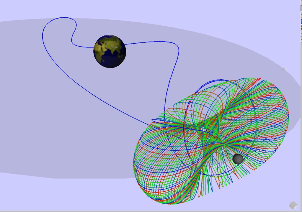
110 Families of Periodic Solutions of the Earth-Moon system. 109

111 The planar Lyapunov family L1. 110

112 The Halo family H1. 111

113 The Halo family H1. 112

114 The Vertical family V1. 113

115 The Axial family A1. 114

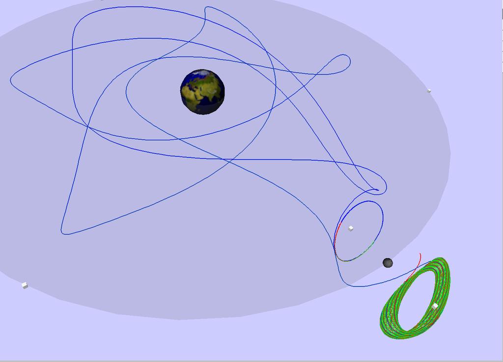
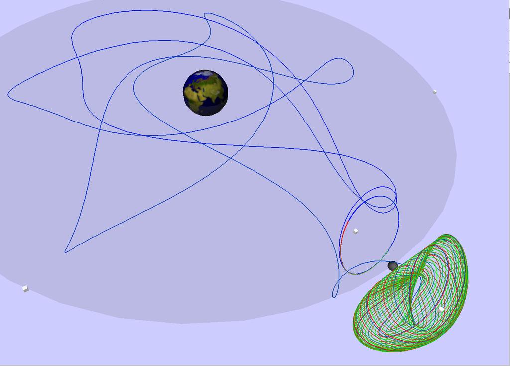
116 Stable and Unstable Manifolds EXAMPLE : Unstable Manifolds in the CR3BP. (Course demo CR3BP/Manifolds ) Small Halo orbits have one real Floquet multiplier outside the unit circle. Such Halo orbits are unstable. They have a 2D unstable manifold. 115

117 The unstable manifold can be computed by continuation. First compute a starting orbit in the manifold. Then continue the orbit keeping, for example, x(1) fixed. 116

118 Continuation, keeping the endpoint x(1) fixed. 117

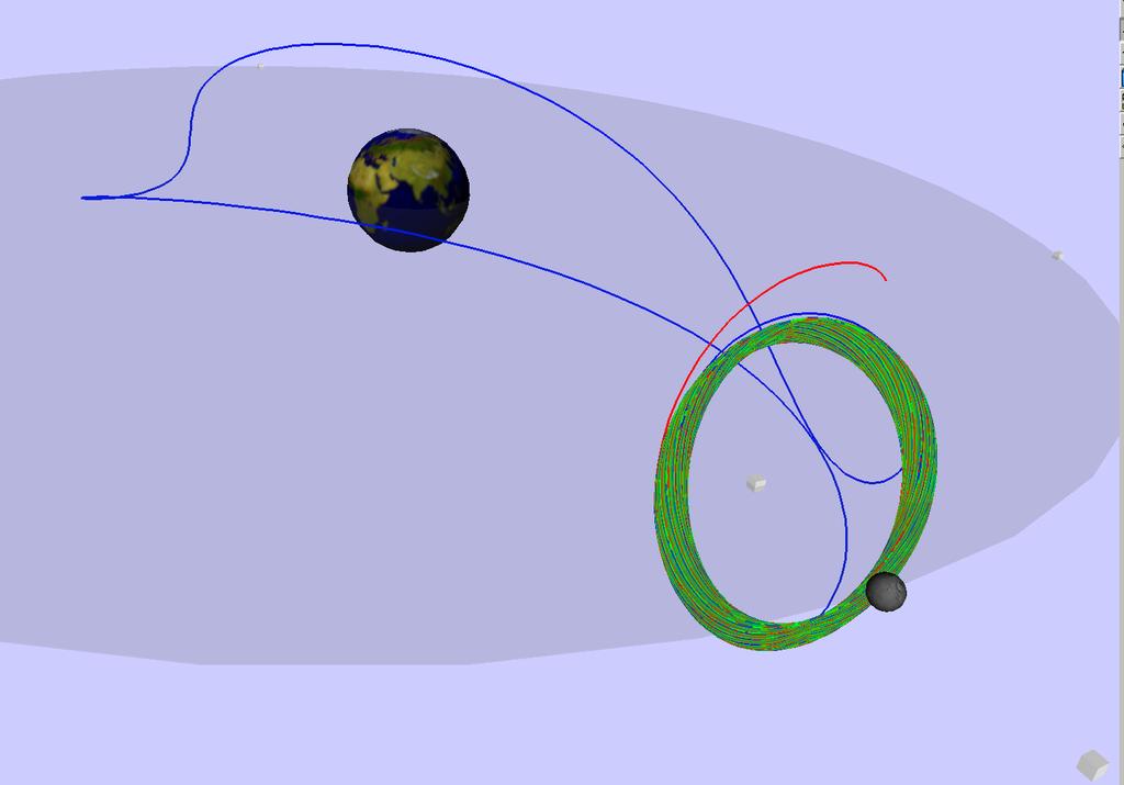
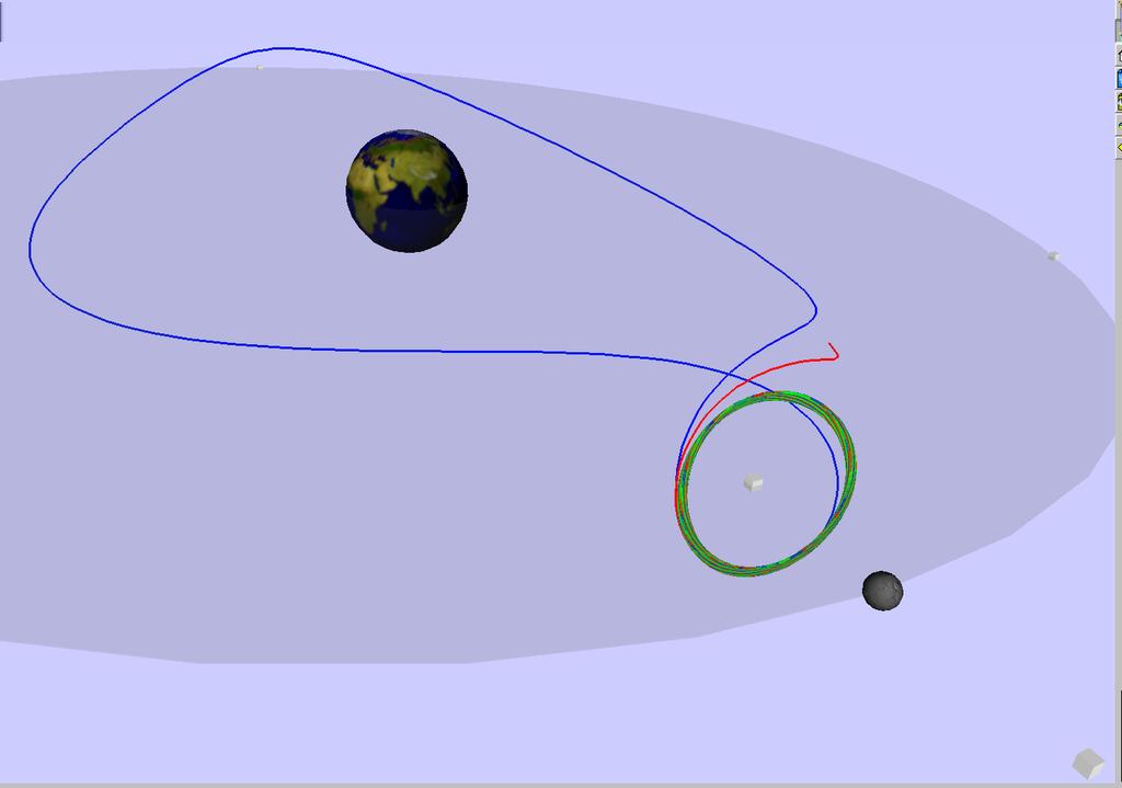
119 The initial orbit can be taken to be much longer Continuation with x(1) fixed can lead to a Halo-to-torus connection! 118

120 119

121 The Halo-to-torus connection can be continued as a solution to F( X k ) = 0, where < X k X k 1, Ẋ k 1 > s = 0. X = ( Halo orbit, Floquet function, connecting orbit). 120

122 In detail, the continuation system is du dτ T uf(u(τ), µ, l) = 0, 1 0 u(1) u(0) = 0, u(τ), u 0 (τ) dτ = 0, dv dτ T ud u f(u(τ), µ, l)v(τ) + λ u v(τ) = 0, v(1) sv(0) = 0 (s = ±1), v(0), v(0) 1 = 0, dw dτ T wf(w(τ), µ, 0) = 0, w(0) (u(0) + εv(0)) = 0, w(1) x x Σ =

123 The system has 18 ODEs, 20 boundary conditions, 1 integral constraint. We need = 4 free parameters. Parameters: An orbit in the unstable manifold: T w, l, T u, x Σ Compute the unstable manifold: T w, l, T u, ε Follow a connecting orbit: λ u, l, T u, ε 122

124 First Example 123

125 124

126 125

127 126

128 127

129 128

130 129

131 130

132 131

133 132

134 133

135 134

136 135

137 136

138 Second Example 137

139 138

140 139

141 140

142 141

143 142

144 143

145 144

146 145

147 146

148 147

149 148

150 149

151 150

152 151

153 152

154 153

155 154

156 155

157 156

158 157

159 158

160 159

161 160

162 161

163 162

164 163

165 164

166 165

167 166

168 167

169 168

170 169

171 170

172 171

173 172

174 173