An Introduction to Numerical Continuation Methods. with Applications. Eusebius Doedel IIMAS-UNAM

Transcription

1 An Introduction to Numerical Continuation Methods with Applications Eusebius Doedel IIMAS-UNAM July 28 - August 1, 2014

2 1 Persistence of Solutions Newton s method for solving a nonlinear equation [B83] 1 G(u) = 0, G( ), u R n, may not converge if the initial guess is not close to a solution. However, one can put a homotopy parameter in the equation. Actually, most equations already have parameters. We will discuss persistence of solutions to such equations. 1 See Page 83 + of the Background Notes on Elementary Numerical Methods.

3 2 The Implicit Function Theorem Let G : R n R R n satisfy (i) G(u 0, λ 0 ) = 0, u 0 R n, λ 0 R. (ii) G u (u 0, λ 0 ) is nonsingular (i.e., u 0 is an isolated solution), (iii) G and G u are smooth near u 0. Then there exists a unique, smooth solution family u(λ) such that G(u(λ), λ) = 0, for all λ near λ 0, u(λ 0 ) = u 0. NOTE : The IFT also holds in more general spaces

4 3 EXAMPLE : A Simple Homotopy. ( Course demo : Simple-Homotopy 2 ) Let g(u, λ) = (u 2 1) (u 2 4) + λ u 2 e 1 10 u. When λ = 0 the equation has four solutions, namely, g(u, 0) = 0, u = ± 1, and u = ± 2. We have g u (u, λ) λ=0 d du (u, λ) λ=0 = 4u 3 10u. 2 doedel/

5 4 Since we have g u (u, 0) = 4u 3 10u, g u ( 1, 0) = 6, g u ( 1, 0) = 6, g u ( 2, 0) = 12, g u ( 2, 0) = 12, which are all nonzero. Thus each of the four solutions when λ = 0 is isolated. Hence each of these solutions persists as λ becomes nonzero, ( at least for small values of λ ).

6 Solution families of g(u, λ) = 0. Note the fold. 5

7 6 NOTE : Each of the four solutions at λ = 0 is isolated. Thus each of these solutions persists as λ becomes nonzero. Only two of the four homotopies reach λ = 1. The other two homotopies meet at a fold. IFT condition (ii) is not satisfied at the fold. (Why not? )

8 7 In the equation let G(u, λ) = 0, u, G(, ) R n, λ R, x ( ) u λ. Then the equation can be written G(x) = 0, G : R n+1 R n. DEFINITION : A solution x 0 of G(x) = 0 is regular if the matrix G 0 x G x (x 0 ), (with n rows and n + 1 columns) has maximal rank, i.e., if Rank(G 0 x) = n.

9 8 In the parameter formulation, G(u, λ) = 0, we have Rank(G 0 x) = Rank(G 0 u G 0 λ) = n (i) G 0 u is nonsingular, or (ii) dim N (G 0 u) = 1, and G 0 λ R(G0 u). Here N (G 0 u) denotes the null space of G 0 u, and R(G 0 u) denotes the range of G 0 u, i.e., R(G 0 u) is the linear space spanned by the n columns of G 0 u.

10 9 COROLLARY (to the IFT) : Let x 0 ( u 0, λ 0 ) be a regular solution of G(x) = 0. Then, near x 0, there exists a unique one-dimensional solution family x(s) with x(0) = x 0. PROOF : Since Rank( G 0 x ) = Rank( G 0 u G 0 λ ) = n, we have that (i) either G 0 u is nonsingular and by the IFT we have u = u(λ) near x 0, (ii) or else we can interchange colums in the Jacobian G 0 x to see that the solution can locally be parametrized by one of the components of u. Thus a (locally) unique solution family passes through x 0. QED!

11 10 NOTE : Such a solution family is sometimes called a solution branch. Case (i) is where the IFT applies directly. Case (ii) is that of a simple fold. Thus even near a simple fold there is a unique solution family. However, near such a fold, the family cannot be parametrized by λ.

12 11 More Examples of IFT Application We give examples where the IFT shows that a given solution persists (at least locally ) when a problem parameter is changed. We also consider cases where the conditions of the IFT are not satisfied.

13 12 EXAMPLE : The A B C Reaction. ( Course demo : Chemical-Reactions/ABC-Reaction/Stationary ) u 1 = u 1 + D(1 u 1 )e u 3, u 2 = u 2 + D(1 u 1 )e u 3 Dσu 2 e u 3, u 3 = u 3 βu 3 + DB(1 u 1 )e u 3 + DBασu 2 e u 3, where 1 u 1 is the concentration of A, u 2 is the concentration of B, u 3 is the temperature, α = 1, σ = 0.04, B = 8, D is the Damkohler number, β > 0 is the heat transfer coefficient. NOTE : The zero stationary solution at D = 0 persists (locally), because the Jacobian is nonsingular there, having eigenvalues 1, 1, and (1 + β).

14 13 Families of stationary solutions of the A B C reaction. (From left to right : β = 1.1, 1.3, 1.5, 1.6, 1.7, 1.8. )

15 14 NOTE : In the preceding bifurcation diagram: u = u u u 2 3. Solid/dashed curves denote stable/unstable solutions. The red squares are Hopf bifurcations. From the basic theory of ODEs: u 0 is a stationary solution of u (t) = f(u(t)) if f(u 0 ) = 0. u 0 is stable if all eigenvalues of f u (u 0 ) are in the negative half-plane. u 0 is unstable if one or more eigenvalues are in the positive half-plane. At a fold there is zero eigenvalue. At a Hopf bifurcation there is a pair of purely imaginary eigenvalues.

16 15 EXAMPLE (of IFT application) : The Gelfand-Bratu Problem. ( Course demo : Gelfand-Bratu/Original ) The boundary value problem u (x) + λ e u(x) = 0, x [0, 1], u(0) = u(1) = 0, defines the stationary states of a solid fuel ignition model. If λ = 0 then u(x) 0 is a solution. This problem can be thought of as an operator equation G(u; λ) = 0. We can use (a generalized) IFT to prove that there is a solution family u = u(λ), for λ small.

17 16 The linearization of G(u; λ) acting on v, i.e., G u (u; λ)v, leads to the homogeneous equation v (x) + λ e u(x) v = 0, v(0) = v(1) = 0, which for the solution u(x) 0 at λ = 0 becomes v (x) = 0, v(0) = v(1) = 0. Since this equation only has the zero solution v(x) 0, the IFT applies. Thus (locally) a unique solution family passes through u(x) 0, λ = 0.

18 17 In Course demo : Gelfand-Bratu/Original the BVP is implemented as a first order system : u 1(t) = u 2 (t), u 2(t) = λ e u1(t), with boundary conditions u 1 (0) = 0, u 1 (1) = 0. A convenient solution measure in the bifurcation diagram is the value of 1 0 u 1 (x) dx.

19 Bifurcation diagram of the Gelfand-Bratu equation. 18

20 Some solutions of the Gelfand-Bratu equation. (The solution at the fold is colored red ). 19

21 20 EXAMPLE : A Boundary Value Problem with Bifurcations. ( Course demo : Basic-BVP/Nonlinear-Eigenvalue ) u + ˆλ u(1 u) = 0, has u(x) 0 as a solution for all ˆλ. u(0) = u(1) = 0, QUESTION : Are there more solutions? Again, this problem corresponds to an operator equation G(u; ˆλ) = 0. Its linearization acting on v leads to the equation G u (u; ˆλ)v = 0, i.e., v + ˆλ (1 2u)v = 0, v(0) = v(1) = 0.

22 21 In particular, the linearization about the zero solution family u 0 is v + ˆλ v = 0, v(0) = v(1) = 0, which for most values of ˆλ only has the zero solution v(x) 0. However, when ˆλ = ˆλ k k 2 π 2, then there are nonzero solutions, namely, v(x) = sin(kπx), Thus the IFT does not apply at ˆλ k = k 2 π 2. (We will see that these solutions are bifurcation points.)

23 22 In the implementation we write the BVP as a first order system. We also use a scaled version of λ. The equations are then u 1 = u 2, u 2 = λ 2 π 2 u 1 (1 u 1 ), with ˆλ = λ 2 π 2. A convenient solution measure in the bifurcation diagram is γ u 2 (0) = u 1(0).

24 Solution families to the nonlinear eigenvalue problem. 23

25 Some solutions to the nonlinear eigenvalue problem. 24

26 25 Hopf Bifurcation THEOREM : Suppose that along a stationary solution family (u(λ), λ), of u = f(u, λ), a complex conjugate pair of eigenvalues α(λ) ± i β(λ), of f u (u(λ), λ) crosses the imaginary axis transversally, i.e., for some λ 0, α(λ 0 ) = 0, β(λ 0 ) 0, and α(λ 0 ) 0. Also assume that there are no other eigenvalues on the imaginary axis. Then there is a Hopf bifurcation, that is, a family of periodic solutions bifurcates from the stationary solution at (u 0, λ 0 ). NOTE : The assumptions imply that fu 0 is nonsingular, so that the stationary solution family is indeed (locally) a function of λ.

27 26 EXAMPLE : The A B C reaction. ( Course demo : Chemical-Reactions/ABC-Reaction/Homoclinic ) A stationary (blue) and a periodic (red) family of the A B C reaction for β = 1.2. The periodic orbits are stable and terminate in a homoclinic orbit.

28 The periodic family orbit family approaching a homoclinic orbit (black). The red dot is the Hopf point; the blue dot is the saddle point on the homoclinic. 27

29 28 Course demo : Chemical-Reactions/ABC-Reaction/Periodic Bifurcation diagram for β = 1.1, 1.3, 1.5, 1.6, 1.7, 1.8. (For periodic solutions u = 1 T T 0 u u u 2 3 dt, where T is the period.)

30 29 EXAMPLE : A Predator-Prey Model. ( Course demo : Predator-Prey/ODE/2D ) u 1 = 3u 1 (1 u 1 ) u 1 u 2 λ(1 e 5u 1 ), u 2 = u 2 + 3u 1 u 2. Here u 1 may be thought of as fish and u 2 as sharks, while the term λ (1 e 5u 1 ), represents fishing, with fishing-quota λ. When λ = 0 the stationary solutions are 3u 1 (1 u 1 ) u 1 u 2 = 0 u 2 + 3u 1 u 2 = 0 (u 1, u 2 ) = (0, 0), (1, 0), ( 1 3, 2).

31 30 The Jacobian matrix is G u (u 1, u 2 ; λ) = ( 3 6u1 u 2 5λe 5u 1 u 1 3u u 1 ) so that G u (0, 0 ; 0) = G u (1, 0 ; 0) = ( ( ) ; real eigenvalues 3, -1 (unstable) ) ; real eigenvalues -3, 2 (unstable) G u ( 1 3, 2 ; 0) = ( ) ; complex eigenvalues 1 2 ± i (stable) All three Jacobians at λ = 0 are nonsingular. Thus, by the IFT, all three stationary points persist for (small) λ 0.

32 31 In this problem we can explicitly find all solutions: Family 1 : (u 1, u 2 ) = (0, 0) Family 2 : u 2 = 0, λ = 3u 1(1 u 1 ) 1 e 5u 1 ( Note that lim u 1 0 λ = lim 3(1 2u 1 ) u 1 0 5e 5u 1 = 3 5 ) Family 3 : u 1 = 1 3, u 2 λ(1 e 5/3 ) = 0 u 2 = 2 3λ(1 e 5/3 ) These solution families intersect at two bifurcation points, one of which is (u 1, u 2, λ) = (0, 0, 3/5).

33 32 fish sharks quota Stationary solution families of the predator-prey model. Solid/dashed curves denote stable/unstable solutions. Note the bifurcations and Hopf bifurcation (red square).

34 fish quota Stationary solution families, showing fish versus quota. Solid/dashed curves denote stable/unstable solutions.

35 34 Stability of Family 1 : ( 3 5λ 0 G u (0, 0 ; λ) = 0 1 ) ; eigenvalues 3 5λ, 1. Hence the zero solution is : and unstable if λ < 3/5, stable if λ > 3/5. Stability of Family 2 : This family has no stable positive solutions.

36 35 Stability of Family 3 : At λ H 0.67 the complex eigenvalues cross the imaginary axis: This crossing is a Hopf bifurcation, Beyond λ H there are stable periodic solutions. Their period T increases as λ increases. The period becomes infinite at λ = λ This final orbit is a heteroclinic cycle.

37 min fish, max fish quota Stationary (blue) and periodic (red) solution families of the predator-prey model. ( For the periodic solution family both the maximum and minimum are shown. )

38 Periodic solutions of the predator-prey model. The largest orbits are close to a heteroclinic cycle. 37

39 38 The bifurcation diagram shows the solution behavior for (slowly) increasing λ : Family 3 is followed until λ H Periodic solutions of increasing period until λ = λ Collapse to trivial solution (Family 1).

40 39 Continuation of Solutions Parameter Continuation Suppose we have a solution (u 0, λ 0 ) of as well as the derivative u 0. G(u, λ) = 0, Here u du dλ. We want to compute the solution u 1 at λ 1 λ 0 + λ.

41 40 "u" u 0 u (0) u 1 u (= du d λ at λ 0 ) λ λ λ 0 1 λ Graphical interpretation of parameter-continuation.

42 41 To solve the equation G(u 1, λ 1 ) = 0, for u 1 (with λ = λ 1 fixed) we use Newton s method G u (u (ν) 1, λ 1 ) u (ν) 1 = G(u (ν) 1, λ 1 ), u (ν+1) 1 = u (ν) 1 + u (ν) 1. ν = 0, 1, 2,. As initial approximation use u (0) 1 = u 0 + λ u 0. If G u (u 1, λ 1 ) is nonsingular, and λ sufficiently small then this iteration will converge [B55].

43 42 After convergence, the new derivative u 1 is computed by solving G u (u 1, λ 1 ) u 1 = G λ (u 1, λ 1 ). This equation is obtained by differentiating with respect to λ at λ = λ 1. G(u(λ), λ) = 0, Repeat the procedure to find u 2, u 3,. NOTE : u 1 can be computed without another LU-factorization of G u (u 1, λ 1 ). Thus the extra work to compute u 1 is negligible.

44 43 EXAMPLE : The Gelfand-Bratu Problem. u (x) + λ e u(x) = 0 for x [0, 1], u(0) = 0, u(1) = 0. We know that if λ = 0 then u(x) 0 is an isolated solution. Discretize by introducing a mesh, 0 = x 0 < x 1 < < x N = 1, x j x j 1 = h, (1 j N), h = 1/N. The discrete equations are : u j+1 2u j + u j 1 h 2 + λ e u j = 0, j = 1,, N 1, with u 0 = u N = 0.

45 44 Let u u 1 u 2 u N 1. Then we can write the discrete equations as G( u, λ ) = 0, where G : R N 1 R R N 1.

46 45 Parameter-continuation : Suppose we have λ 0, u 0, and u 0. Set λ 1 = λ 0 + λ. Newton s method : for ν = 0, 1, 2,, with G u (u (ν) 1, λ 1 ) u (ν) 1 = G(u (ν) 1, λ 1 ), u (ν+1) 1 = u (ν) 1 + u (ν) 1, u (0) 1 = u 0 + λ u 0. After convergence compute u 1 from G u (u 1, λ 1 ) u 1 = G λ (u 1, λ 1 ). Repeat the procedure to find u 2, u 3,.

47 46 Here G u ( u, λ ) = 2 h 2 + λe u 1 1 h λe u h 2 h h h 2 2 h 2 + λe u N 1. Thus we must solve a tridiagonal system for each Newton iteration. NOTE : The solution family has a fold where parameter-continuation fails! A better continuation method is pseudo-arclength continuation. There are also better discretizations, namely collocation, as used in AUTO.

48 47 Pseudo-Arclength Continuation This method allows continuation of a solution family past a fold. It was introduced by H. B. Keller ( ) in Suppose we have a solution (u 0, λ 0 ) of G( u, λ ) = 0, as well as the normalized direction vector ( u 0, λ 0 ) of the solution family. Pseudo-arclength continuation consists of solving these equations for (u 1, λ 1 ) : G(u 1, λ 1 ) = 0, u 1 u 0, u 0 + (λ 1 λ 0 ) λ 0 s = 0.

49 48 "u" u 0 u 1 u 0 s 01 λ ( u, ) 0 λ 0 λ 0 λ 1 λ Graphical interpretation of pseudo-arclength continuation.

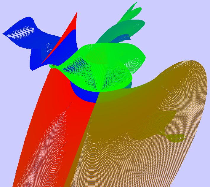
50 49 Solve the equations G(u 1, λ 1 ) = 0, u 1 u 0, u 0 + (λ 1 λ 0 ) λ 0 s = 0. for (u 1, λ 1 ) by Newton s method : (G1 u) (ν) u 0 (G 1 λ )(ν) λ 0 ( (ν) ) u 1 λ (ν) 1 = G(u (ν) 1, λ (ν) 1 ) u (ν) 1 u 0, u 0 + (λ (ν) 1 λ 0 ) λ 0 s. Compute the next direction vector by solving and normalize it. G1 u u 0 G 1 λ λ 0 ( u1 λ 1 ) = 0, 1

51 50 NOTE : We can compute ( u 1, λ 1 ) with only one extra backsubstitution. The orientation of the family is preserved if s is sufficiently small. Rescale the direction vector so that indeed u λ 2 1 = 1.

52 51 FACT : The Jacobian is nonsingular at a regular solution. ( ) u PROOF : Let x R λ n+1. Then pseudo-arclength continuation can be simply written as G(x 1 ) = 0, x 1 x 0, ẋ 0 s = 0, ( ẋ 0 = 1 ). x 0 s x 1 x 0 Pseudo-arclength continuation.

53 52 The pseudo-arclength equations are G(x 1 ) = 0, x 1 x 0, ẋ 0 s = 0, ( ẋ 0 = 1 ). The Jacobian matrix in Newton s method at s = 0 is ( ) G 0 x. ẋ 0 At a regular solution N (G 0 x) = Span{ẋ 0 }. We must show that ( ) G 0 x ẋ 0 is nonsingular at a regular solution.

54 53 If on the contrary ( ) G 0 x ẋ 0 is singular then for some vector z 0 we have : G 0 x z = 0, ẋ 0, z = 0, Since by assumption N (G 0 x) = Span{ẋ 0 }, we have z = c ẋ 0, for some constant c. But then 0 = ẋ 0, z = c ẋ 0, ẋ 0 = c ẋ 0 2 = c, so that z = 0, which is a contradiction. QED!

55 54 EXAMPLE : The Gelfand-Bratu Problem. Use pseudo-arclength continuation for the discretized Gelfand-Bratu problem. Then the matrix ( ) Gx ẋ = ( ) Gu G λ u λ, in Newton s method is a bordered tridiagonal matrix :. which can be decomposed very efficiently.

56 55 Following Folds and Hopf Bifurcations At a fold the the behavior of a system can change drastically. How does the fold location change when a second parameter varies? Thus we want the compute a locus of folds in 2 parameters. We also want to compute loci of Hopf bifurcations in 2 parameters.

57 56 Following Folds Treat both parameters λ and µ as unknowns, and compute a solution family X(s) ( u(s), φ(s), λ(s), µ(s) ), to F(X) G(u, λ, µ) = 0, G u (u, λ, µ) φ = 0, φ, φ 0 1 = 0, and the added continuation equation u u 0, u 0 + φ φ 0, φ0 + (λ λ 0 ) λ 0 + (µ µ 0 ) µ 0 s = 0. As before, ( u 0, φ0, λ0, µ 0 ), is the direction of the family at the current solution point ( u 0, φ 0, λ 0, µ 0 ).

58 57 EXAMPLE : The A B C Reaction. ( Course demo : Chemical-Reactions/ABC-Reaction/Folds-SS ) The equations are u 1 = u 1 + D(1 u 1 )e u 3, u 2 = u 2 + D(1 u 1 )e u 3 Dσu 2 e u 3, u 3 = u 3 βu 3 + DB(1 u 1 )e u 3 + DBασu 2 e u 3, where 1 u 1 is the concentration of A, u 2 is the concentration of B, u 3 is the temperature, α = 1, σ = 0.04, B = 8, D is the Damkohler number, β is the heat transfer coefficient.

59 58 A stationary solution family for β = Note the two folds and the Hopf bifurcation.

60 β β D D A locus of folds (with blow-up) for the A B C reaction. Notice the two cusp singularities along the 2-parameter locus. ( There is a swallowtail singularity in nearby 3-parameter space. )

61 u D Stationary solution families for β = 1.20, 1.21,, ( Open diamonds mark folds, solid red squares mark Hopf points. )

62 61 Following Hopf Bifurcations The extended system is f(u, λ, µ) = 0, F(u, φ, β, λ; µ) f u (u, λ, µ) φ i β φ = 0, φ, φ 0 1 = 0, where F : R n C n R 2 R R n C n C, and to which we want to compute a solution family ( u, φ, β, λ, µ ), with u R n, φ C n, β, λ, µ R. Above φ 0 belongs to a reference solution ( u 0, φ 0, β 0, λ 0, µ 0 ), which normally is the latest computed solution along a family.

63 62 EXAMPLE : The A B C Reaction. ( Course demo : Chemical-Reactions/ABC-Reaction/Hopf ) The stationary family with Hopf bifurcation for β = 1.20.

64 β D The locus of Hopf bifurcations for the A B C reaction.

65 u D Stationary solution families for β = 1.20, 1.20, 1.25, 1.30,, 2.30, with Hopf bifurcations (the red squares).

66 65 Boundary Value Problems Consider the first order system of ordinary differential equations u (t) f( u(t), µ, λ ) = 0, t [0, 1], where u( ), f( ) R n, λ R, µ R nµ, subject to boundary conditions b( u(0), u(1), µ, λ ) = 0, b( ) R n b, and integral constraints 1 0 q( u(s), µ, λ ) ds = 0, q( ) R nq.

67 66 This boundary value problem (BVP) is of the form where F( X ) = 0, X = ( u, µ, λ ), to which we add the continuation equation X X 0, Ẋ 0 s = 0, where X 0 represents the latest solution computed along the family. In detail, the continuation equation is 1 0 u(t) u 0 (t), u 0 (t) dt + µ µ 0, µ 0 + (λ λ 0 ) λ 0 s = 0.

68 67 NOTE : In the context of continuation we solve this BVP for (u( ), λ, µ). In order for problem to be formally well-posed we must have n µ = n b + n q n 0. A simple case is n q = 0, n b = n, for which n µ = 0.

69 68 Discretization: Orthogonal Collocation Introduce a mesh { 0 = t 0 < t 1 < < t N = 1 }, where h j t j t j 1, (1 j N), Define the space of (vector) piecewise polynomials P m h as P m h { p h C[0, 1] : p h [tj 1,t j ] P m }, where P m is the space of (vector) polynomials of degree m.

70 69 The collocation method consists of finding p h P m h, µ R nµ, such that the following collocation equations are satisfied : p h(z j,i ) = f( p h (z j,i ), µ, λ ), j = 1,, N, i = 1,, m, and such that p h satisfies the boundary and integral conditions. The collocation points z j,i in each subinterval [ t j 1, t j ], are the (scaled) roots of the mth-degree orthogonal polynomial (Gauss points 3 ). 3 See Pages 261, 287 of the Background Notes on Elementary Numerical Methods.

71 t t t t N t j-1 t j z j,1 z j,2 z j,3 t j-1 t j t j-2/3 t j-1/3 lj,3(t) lj,1(t) The mesh {0 = t 0 < t 1 < < t N = 1}, with collocation points and extended-mesh points shown for m = 3. Also shown are two of the four local Lagrange basis polynomials.

72 71 Since each local polynomial is determined by (m + 1) n, coefficients, the total number of unknowns (considering λ as fixed) is (m + 1) n N + n µ. This is matched by the total number of equations : collocation : m n N, continuity : (N 1) n, constraints : n b + n q ( = n + n µ ).

73 72 Assume that the solution u(t) of the BVP is sufficiently smooth. Then the order of accuracy of the orthogonal collocation method is m, i.e., p h u = O(h m ). At the main meshpoints t j we have superconvergence : max j p h (t j ) u(t j ) = O(h 2m ). The scalar variables λ and µ are also superconvergent.

74 73 Implementation For each subinterval [ t j 1, t j ], introduce the Lagrange basis polynomials { l j,i (t) }, j = 1,, N, i = 0, 1,, m, defined by where l j,i (t) = t j i m m k=0,k i t j i m t t j k m t j i m h j. t j k m The local polynomials can then be written m p j (t) = l j,i (t) u j i. m With the above choice of basis i=0, u j u(t j ) and u j i m where u(t) is the solution of the continuous problem. u(t j i ), m

75 74 The collocation equations are p j(z j,i ) = f( p j (z j,i ), µ, λ ), i = 1,, m, j = 1,, N. The boundary conditions are b i ( u 0, u N, µ, λ ) = 0, i = 1,, n b. The integral constraints can be discretized as N m j=1 i=0 ω j,i q k ( u j i m, µ, λ) = 0, k = 1,, n q, where the ω j,i are the Lagrange quadrature weights.

76 75 The continuation equation is 1 0 u(t) u 0 (t), u 0 (t) dt + µ µ 0, µ 0 + (λ λ 0 ) λ 0 s = 0, where ( u 0, µ 0, λ 0 ), is the previous solution along the solution family, and ( u 0, µ 0, λ0 ), is the normalized direction of the family at the previous solution. The discretized continuation equation is of the form N j=1 m i=0 ω j,i u j i m (u 0 ) j i m, ( u 0 ) j i m + µ µ 0, µ 0 + (λ λ 0 ) λ 0 s = 0.

77 76 Numerical Linear Algebra The complete discretization consists of m n N + n b + n q + 1, nonlinear equations, with unknowns {u j i } R mnn+n, µ R nµ, λ R. m These equations are solved by a Newton-Chord iteration.

78 77 We illustrate the numerical linear algebra for the case n = 2 ODEs, N = 4 mesh intervals, m = 3 collocation points, n b = 2 boundary conditions, n q = 1 integral constraint, and the continuation equation. The operations are also done on the right hand side, which is not shown. Entries marked have been eliminated by Gauss elimination. Entries marked denote fill-in due to pivoting. Most of the operations can be done in parallel.

79 78 u 0 u 1 3 u 2 3 u 1 u 2 u 3 u N µ λ The structure of the Jacobian.

80 79 u 0 u 1 3 u 2 3 u 1 u 2 u 3 u N µ λ The system after condensation of parameters, which can be done in parallel.

81 80 u 0 u 1 3 u 2 3 u 1 u 2 u 3 u N µ λ The preceding matrix, showing the decoupled subsystem.

82 81 u 0 u 1 3 u 2 3 u 1 u 2 u 3 u N µ λ Stage 1 of the nested dissection to solve the decoupled subsystem.

83 82 u 0 u 1 3 u 2 3 u 1 u 2 u 3 u N µ λ Stage 2 of the nested dissection to solve the decoupled subsystem.

84 83 u 0 u 1 3 u 2 3 u 1 u 2 u 3 u N µ λ The preceding matrix showing the final decoupled subsystem.

85 84 u 0 u 1 3 u 2 3 u 1 u 2 u 3 u N µ λ A A B B A A B B The approximate Floquet multipliers are the eigenvalues of M B 1 A.

86 85 Accuracy Test The Table shows the location of the fold in the Gelfand-Bratu problem, for 4 Gauss collocation points per mesh interval, and N mesh intervals. N Fold location

87 86 Periodic Solutions Periodic solutions can be computed efficiently using a BVP approach. This method also determines the period very accurately. Moreover, the technique can compute unstable periodic orbits.

88 87 Consider u (t) = f( u(t), λ ), u( ), f( ) R n, λ R. Fix the interval of periodicity by the transformation t t T. Then the equation becomes u (t) = T f( u(t), λ ), u( ), f( ) R n, T, λ R. and we seek solutions of period 1, i.e., u(0) = u(1). Note that the period T is one of the unknowns.

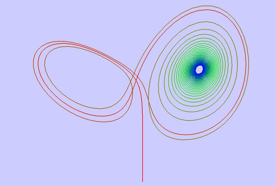
89 88 The above equations do not uniquely specify u and T : Assume that we have computed ( u k 1 ( ), T k 1, λ k 1 ), and we want to compute the next solution ( u k ( ), T k, λ k ). Then u k (t) can be translated freely in time : If u k (t) is a periodic solution, then so is u k (t + σ), for any σ. Thus, a phase condition is needed.

90 89 An example is the Poincaré phase condition u k (0) u k 1 (0), u k 1(0) = 0. ( But we will derive a numerically more suitable integral phase condition. ) u k-1 (0) u k-1 (0) u (0) k Graphical interpretation of the Poincaré phase condition.

91 90 An Integral Phase Condition If ũ k (t) is a solution then so is for any σ. ũ k (t + σ), We want the solution that minimizes D(σ) 1 0 ũ k (t + σ) u k 1 (t) 2 2 dt. The optimal solution ũ k (t + ˆσ), must satisfy the necessary condition D (ˆσ) = 0.

92 91 Differentiation gives the necessary condition Writing 1 0 ũ k (t + ˆσ) u k 1 (t), ũ k(t + ˆσ dt = 0. u k (t) ũ k (t + ˆσ), gives 1 0 u k (t) u k 1 (t), u k(t) dt = 0. Integration by parts, using periodicity, gives 1 u 0 k (t), u k 1 (t) dt = 0. This is the integral phase condition.

93 92 Continuation of Periodic Solutions Pseudo-arclength continuation is used to follow periodic solutions. It allows computation past folds along a family of periodic solutions. It also allows calculation of a vertical family of periodic solutions. For periodic solutions the continuation equation is 1 0 u k (t) u k 1 (t), u k 1 (t) dt + (T k T k 1 ) T k 1 + (λ k λ k 1 ) λ k 1 = s.

94 93 SUMMARY : We have the following equations for periodic solutions : u k(t) = T f( u k (t), λ k ), u k (0) = u k (1), 1 0 u k (t), u k 1(t) dt = 0, with continuation equation 1 0 u k (t) u k 1 (t), u k 1 (t) dt + (T k T k 1 ) T k 1 + (λ k λ k 1 ) λ k 1 = s, where u( ), f( ) R n, λ, T R.

95 94 Stability of Periodic Solutions In our continuation context, a periodic solution of period T satisfies u (t) = T f( u(t)), for t [0, 1], u(0) = u(1), (for given value of the continuation parameter λ). A small perturbation in the initial condition u(0) + ɛ v(0), ɛ small, leads to the linearized equation v (t) = T f u ( u(t) ) v(t), for t [0, 1], which induces a linear map v(0) v(1), represented by v(1) = M v(0).

96 95 v(1) = M v(0) The eigenvalues of M are the Floquet multipliers that determine stability. M always has a multiplier µ = 1, since differentiating u (t) = T f( u(t)), gives where v (t) = T f u ( u(t) ) v(t), v(t) = u (t), with v(0) = v(1).

97 96 v(1) = M v(0) If M has a Floquet multiplier µ with µ > 1 then u(t) is unstable. If all multipliers (other than µ = 1) satisfy µ < 1 then u(t) is stable. At folds and branch points there are two multipliers µ = 1. At a period-doubling bifurcation there is a real multiplier µ = 1. At a torus bifurcation there is a complex pair on the unit circle.

98 97 EXAMPLE : The Lorenz Equations. ( Course demo : Lorenz ) These equations were introduced in 1963 by Edward Lorenz ( ) as a simple model of atmospheric convection : x = σ (y x), y = ρ x y x z, z = x y β z, where (often) σ = 10, β = 8/3, ρ = 28.

99 98 Course demo : Lorenz/Basic Bifurcation diagram of the Lorenz equations for σ = 10 and β = 8/3.

100 99 Course demo : Lorenz/Basic Unstable periodic orbits of the Lorenz equations.

101 100 In the Lorenz Equations : The zero stationary solution is unstable for ρ > 1. Two nonzero stationary families bifurcate at ρ = 1. The nonzero stationary solutions are unstable for ρ > ρ H. At ρ H 24.7 there are Hopf bifurcations. Unstable periodic solution families emanate from the Hopf bifurcations. These families end in homoclinic orbits (infinite period) at ρ At ρ = 28 (and a range of other values) there is the Lorenz attractor.

102 101 EXAMPLE : The A B C Reaction. ( Course demo : Chemical-Reactions/ABC-Reaction/Periodic ) Stationary and periodic solution families of the A B C reaction: β = Note the coexistence of stable solutions, for example, solutions 1 and 2.

103 max u3 6 5 max u D D max u3 6 5 max u D D Top left: β = 1.55, right: β = 1.56, Bottom left: β = 1.57, right: β = ( QUESTION : Is something missing somewhere? )

104 103 Following Folds for Periodic Solutions Recall that periodic orbits families can be computed using the equations u (t) T f( u(t), λ ) = 0, u(0) u(1) = 0, 1 0 u(t), u 0(t) dt = 0, where u 0 is a reference orbit, typically the latest computed orbit. The above boundary value problem is of the form where F( X, λ ) = 0, X = ( u, T ).

105 104 At a fold with respect to λ we have F X ( X, λ ) Φ = 0, where Φ, Φ = 1, X = ( u, T ), Φ = ( v, S ), i.e., the linearized equations about X have a nonzero solution Φ. In detail : v (t) T f u ( u(t), λ ) v S f( u(t), λ ) = 0, v(0) v(1) = 0, 1 0 v(t), u 0(t) dt = 0, 1 0 v(t), v(t) dt + S 2 = 1.

106 105 The complete extended system to follow a fold is F( X, λ, µ ) = 0, F X ( X, λ, µ ) Φ = 0, Φ, Φ 1 = 0, with two free problem parameters λ and µ. To the above we add the continuation equation X X 0, Ẋ 0 + Φ Φ 0, Φ0 + (λ λ 0 ) λ 0 + (µ µ 0 ) µ 0 s = 0.

107 106 In detail : u (t) T f( u(t), λ, µ ) = 0, 1 0 u(0) u(1) = 0, u(t), u 0(t) dt = 0, v (t) T f u ( u(t), λ, µ ) v S f( u(t), λ, µ ) = 0, with normalization v(0) v(1) = 0, v(t), u 0(t) dt = 0, 0 v(t), v(t) dt + S 2 1 = 0, and continuation equation 1 0 u(t) u 0 (t), u 0 (t) dt v(t) v 0 (t), v 0 (t) dt + + (T 0 T ) T 0 + (S 0 S)Ṡ0 + (λ λ 0 ) λ 0 + (µ µ 0 ) µ 0 s = 0.

108 107 EXAMPLE : The A B C Reaction. ( Course demo : Chemical-Reactions/ABC-Reaction/Folds-PS ) Stationary and periodic solution families of the A B C reaction. (with blow-up) for β = Note the three folds, labeled 1, 2, 3.

109 β D Loci of folds along periodic solution families for the A B C reaction.

110 Stationary and periodic solution families of the A B C reaction: β =

111 max u D Stationary and periodic solution families of the A B C reaction: β = 1.57.

112 Stationary and periodic solution families of the A B C reaction: β =

113 Stationary and periodic solution families of the A B C reaction: β =

114 Stationary and periodic solution families of the A B C reaction: β =

115 Periodic solutions along the isola for β = (Stable solutions are blue, unstable solutions are red.) 114

116 115 Following Period-doubling Bifurcations Let ( u(t), T ) be a periodic solution, i.e., a solution of u (t) T f( u(t), λ ) = 0, 1 where u 0 is a reference orbit. 0 u(0) u(1) = 0, u(t), u 0(t) dt = 0, A necessary condition for a period-doubling bifurcation is that the following linearized system have a nonzero solution v(t) : v (t) T f u ( u(t), λ ) v(t) = 0, 1 0 v(0) + v(1) = 0, v(t), v(t) dt = 1.

117 116 The complete extended system to follow a period-doubling bifurcation is u (t) T f( u(t), λ, µ ) = 0, 1 0 u(0) u(1) = 0, u(t), u 0(t) dt = 0, v (t) T f u ( u(t), λ ) v(t) = 0, 1 and continuation equation 1 0 u(t) u 0 (t), u 0 (t) dt + 0 v(0) + v(1) = 0, v(t), v(t) dt 1 = 0, 1 0 v(t) v 0 (t), v 0 (t) dt + + (T 0 T ) T 0 + (λ λ 0 ) λ 0 + (µ µ 0 ) µ 0 s = 0.

118 117 EXAMPLE : Period-Doubling Bifurcations in the Lorenz Equations. ( Course demo : Lorenz/Period-Doubling ) The Lorenz equations also have period-doubling bifurcations. In fact, there is a period-doubling cascade for large ρ. We start from numerical data. (Such data may be from simulation, i.e., initial value integration.) We also want to compute loci of period-doubling bifurcations.

119 118 ( Course demo : Lorenz/Period-Doubling ) Left panel : Solution families of the Lorenz equations. The open diamonds denote period-doubling bifurcations. Right panel : Solution 1 was found by initial value integration.

120 119 ( Course demo : Lorenz/Period-Doubling ) Left panel : Right panel : A primary period-doubled solution. A secondary period-doubled solution.

121 120 ( Course demo : Lorenz/Period-Doubling ) Loci of period-doubling bifurcations for the Lorenz equations (with blow-up). Black: primary, Red: secondary, Blue: tertiary period-doublings.

122 121 Periodic Solutions of Conservative Systems EXAMPLE : A Model Conservative System. ( Course demo : Vertical-HB ) u 1 = u 2, u 2 = u 1 (1 u 1 ). PROBLEM : This system has a family of periodic solutions, but no parameter! The system has a constant of motion, namely the Hamiltonian H(u 1, u 2 ) = 1 2 u u u3 1.

123 122 REMEDY : Introduce an unfolding term with unfolding parameter λ : u 1 = λ u 1 u 2, u 2 = u 1 (1 u 1 ). Then there is a vertical Hopf bifurcation from the trivial solution at λ = 0.

124 Bifurcation diagram of the vertical Hopf bifurcation problem. ( Course demo : Vertical-HB ) 123

125 124 NOTE : The family of periodic solutions is vertical. The parameter λ is solved for in each continuation step. Upon solving, λ is found to be zero, up to numerical precision. One can use standard BVP continuation and bifurcation algorithms.

126 A phase plot of some periodic solutions. 125

127 126 EXAMPLE : The Circular Restricted 3-Body Problem (CR3BP). ( Course demo : Restricted-3Body/Earth-Moon/Orbits ) x = 2y + x y = 2x + y z (1 µ) z = r1 3 (1 µ) (x + µ) r 3 1 (1 µ) y r 3 1 µ z r 3 2, µ y r 3 2 µ (x 1 + µ) r 3 2,, where r 1 = (x + µ) 2 + y 2 + z 2, r 2 = (x 1 + µ) 2 + y 2 + z 2. and ( x, y, z ) denotes the position of the zero-mass body. NOTE : For the Earth-Moon system µ

128 127 The CR3BP has one integral of motion, namely, the Jacobi-constant : J = x 2 + y 2 + z 2 2 U(x, y, z) µ 1 µ 2, where and U = 1 2 (x2 + y 2 ) + 1 µ r 1 + µ r 2, r 1 = (x + µ) 2 + y 2 + z 2, r 2 = (x 1 + µ) 2 + y 2 + z 2.

129 128 Boundary value formulation : x = T v x y = T v y z = T v z v x = T [ 2v y + x (1 µ)(x + µ)r1 3 µ(x 1 + µ)r2 3 + λ v x ] v y = T [ 2v x + y (1 µ)yr1 3 µyr2 3 + λ v y ] v z = T [ (1 µ)zr1 3 µzr2 3 + λ v z ] with periodicity boundary conditions x(1) = x(0), y(1) = y(0), z(1) = z(0), v x (1) = v x (0), v y (1) = v y (0), v z (1) = v z (0), + phase constraint + continuation equation. Here T is the period of the orbit.

130 129 NOTE : One can use BVP continuation and bifurcation algorithms. The unfolding term λ v regularizes the continuation. λ will be zero, once solved for. Other unfolding terms are possible.

131 Schematic bifurcation diagram of periodic solution families of the Earth-Moon system. 130

132 The planar Lyapunov family L1. 131

133 The Halo family H1. 132

134 The Halo family H1. 133

135 The Vertical family V1. 134

136 The Axial family A1. 135

137 136 Stable and Unstable Manifolds EXAMPLE : Phase-plane orbits: Fixed length. These can be computed by orbit continuation. Model equations are x = ɛx y 3, where ɛ > 0 is small. y = y + x 3. There is only one equilibrium, namely, (x, y) = (0, 0). This equilibrium has eigenvalues ɛ and 1 ; it is a source.

138 137 For the computations : The time variable t is scaled to [0, 1]. The actual integration time T is then an explicit parameter : x = T ( ɛx y 3 ), y = T ( y + x 3 ).

139 138 These constraints are used : To put the initial point on a small circle around the origin : x(0) r cos(2πθ) = 0, y(0) r sin(2πθ) = 0. To keep track of the end points : x(1) x 1 = 0, y(1) y 1 = 0. To keep track of the length of the orbits 1 0 x (t) 2 + y (t) 2 dt L = 0.

140 139 The computations are done in 3 stages : In the first run an orbit is grown by continuation : - The free parameters are T, L, x 1, y 1. - The starting point is on the small circle of radius r. - The starting point is in the strongly unstable direction. - The value of ɛ is 0.5 in the first run. In the second run the value of ɛ is decreased to 0.01 : - The free parameters are ɛ, T, x 1, y 1. In the third run the initial point is free to move around the circle : - The free parameters are θ, T, x 1, y 1.

141 140 ( Course demo : Basic-Manifolds/2D-ODE/Fixed-Length ) Unstable Manifolds in the Plane: Orbits of Fixed Length. (The right-hand panel is a blow-up, and also shows fewer orbits.)

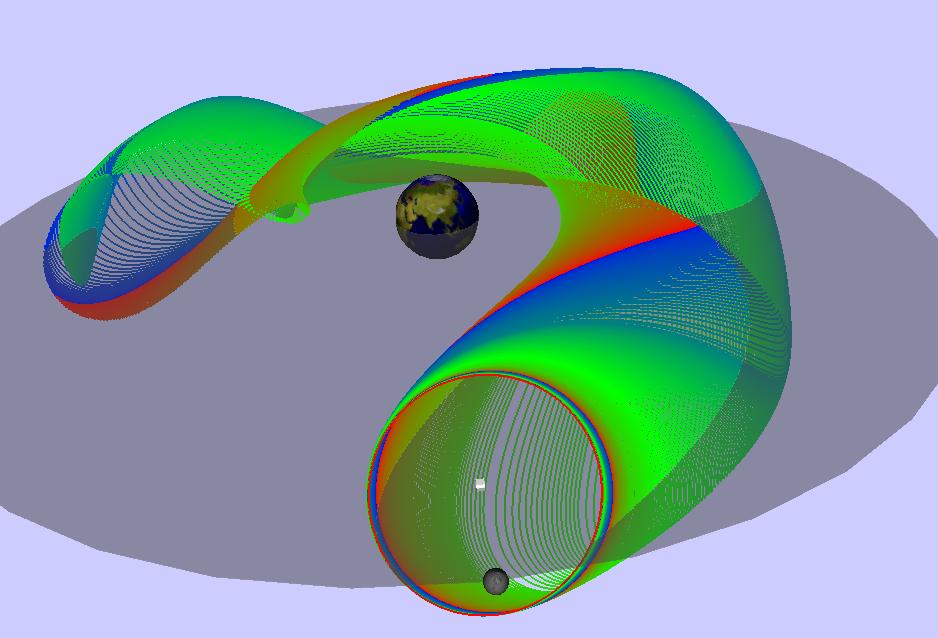
142 141 EXAMPLE : Phase-plane orbits: Variable length. These can also be computed by orbit continuation. Model equations are x = ɛx y 2, y = y + x 2. The origin (x, y) = (0, 0) is an equilibrium. The origin has eigenvalues ɛ and 1 ; it is a source. Thus the origin has a 2-dimensional unstable manifold. We compute this stable manifold using continuation. (The equations are 2D; so we actually compute a phase portrait.)

143 142 For the computations : The time variable t is scaled to [0, 1]. The actual integration time T is then an explicit parameter : x = T (ɛx y 2 ), y = T (y + x 2 ). NOTE : There is also a nonzero equilibrium (x, y) = (ɛ 1 3, ɛ 2 3 ). It is a saddle (1 positive, 1 negative eigenvalue).

144 143 These constraints are used : To put the initial point on a small circle at the origin : x(0) r cos(2πθ) = 0, y(0) r sin(2πθ) = 0. To keep track of the end points : x(1) x 1 = 0, y(1) y 1 = 0. To keep track of the length of the orbits we add an integral constraint : 1 0 x (t) 2 + y (t) 2 dt L = 0. To allow the length L to contract : (T max T )(L max L) c = 0.

145 144 Again the computations are done in 3 stages : In the first run an orbit is grown by continuation : - The free parameters are T, L, x 1, y 1, c. - The starting point is on a small circle of radius r. - The starting point is in the strongly unstable direction. - In this first run ɛ = 0.5. In the second run the value of ɛ is decreased to 0.05 : - The free parameters are ɛ, T, L, x 1, y 1. In the third run the initial point is free to move around the circle : - The free parameters are θ, T, L, x 1, y 1.

146 145 ( Course demo : Basic-Manifolds/2D-ODE/Variable-Length ) Unstable Manifolds in the Plane: Orbits of Variable Length.

147 146 ( Course demo : Basic-Manifolds/2D-ODE/Variable-Length ) Unstable Manifolds in the Plane: Orbits of Variable Length (Blow-up).

148 147 EXAMPLE : A 2D unstable manifold in R 3. This can also be computed by orbit continuation. The model equations are x = ɛx z 3, y = y x 3, z = z + x 2 + y 2. We take ɛ = The origin is a saddle with eigenvalues ɛ, 1, and 1. Thus the origin has a 2-dimensional unstable manifold. The initial point moves around a circle in the 2D unstable eigenspace. The equations are 3D; so we will compute a 2D manifold in R 3. There is also a nonzero saddle, so we use retraction. The set-up is similar to the 2D phase-portrait example.

149 148 ( Course demo : Basic-Manifolds/3D-ODE/Variable-Length ) Unstable Manifolds in R 3 : Orbits of Variable Length.

150 149 EXAMPLE : Another 2D unstable manifold in R 3. The model equations are x = ɛx y 3 + z 3, y = y + x 3 + z 3, z = z x 2 + y 2. We take ɛ = The origin is a saddle with eigenvalues ɛ, 1, and 1. Thus the origin has a 2-dimensional unstable manifold. The initial point moves around a circle in the 2D unstable eigenspace. The equations are 3D; so we will compute a 2D manifold in R 3. No retraction is needed, so we choose to compute orbits of fixed length. The set-up is similar to the 2D phase-portrait example.

151 150 ( Course demo : Basic-Manifolds/3D-ODE/Fixed-Length ) Unstable Manifolds in R 3 : Orbits of Fixed Length.

152 151 The Lorenz Manifold For ρ > 1 the origin is a saddle point. The Jacobian has two negative and one positive eigenvalue. The two negative eigenvalues give rise to a 2D stable manifold. This manifold is known as as the Lorenz Manifold. The set-up is as for the earlier 3D model, using fixed length.

153 152 Course demo : Lorenz/Manifolds/Origin/Fixed-Length Part of the Lorenz Manifold (with blow-up). Orbits have fixed length L = 60.

154 153 Course demo : Lorenz/Manifolds/Origin/Fixed-Length Part of the Lorenz Manifold. Orbits have fixed length L = 200.

155 154 Heteroclinic Connections. The Lorenz Manifold helps understand the Lorenz attractor. Many orbits in the manifold depend sensitively on initial conditions. During the manifold computation one can locate heteroclinic orbits. These are also in the 2D unstable manifold of the nonzero equilibria. The heteroclinic orbits have a combinatorial structure 4. One can also continue heteroclinic orbits as ρ varies. 4 Nonlinearity 19, 2006,

156 155 Course demo : Lorenz/Heteroclinics Four heteroclinic orbits with very close initial conditions

157 156 One can also determine the intersection of the Lorenz manifold with a sphere. The set-up is as follows : x = T σ (y x), y = T (ρ x y x z), z = T (x y β z), which is of the form u (t) = T f( u(t) ), for 0 t 1, where T is the actual integration time, which is negative! To this we add boundary and integral constraints.

158 157 The complete set-up consists of the ODE u (t) = T f( u(t) ), for 0 t 1, subject to the following constraints : u(0) ɛ (cos(θ) v 1 sin(θ) v 2 ) = 0 u(0) is on a small circle u(1) u 1 = 0 to keep track of the end point u(1) u 1 R = 0 distance of u 1 to the origin u 1 / u 1, f(u 1 )/ f(u 1 ) τ = 0 to locate tangencies, where τ = 0 T 1 0 f(u) ds L = 0 to keep track of the orbit length (T T n ) (L L n ) c = 0. allows retraction into the sphere

159 158 The continuation system has the form F(X k ) = 0, where X = ( u( ), Λ ). with continuation equation X k X k 1, Ẋ k 1 s = 0, ( Ẋk 1 = 1 ). The computations are done in 2 stages : In the first run an orbit is grown by continuation : - The starting point is on the small circle of radius ɛ. - The starting point is in the strongly stable direction. - The free parameters are Λ = (T, L, c, τ, R, u 1 ). In the second run the orbit sweeps the stable manifold. - The initial point is free to move around the circle : - The free parameters are Λ = (T, L, θ, τ, R, u 1 ).

160 159 Course demo : Lorenz/Manifolds/Origin/Sphere Intersection of the Lorenz Manifold with a sphere

161 160 NOTE : We do not just change the initial point (i.e., θ) and integrate! Every continuation step requires solving a boundary value problem. The continuation stepsize s controls the change in X. X can only change a little in any continuation step. This way the entire manifold (up to a given length L) is computed. The retraction constraint allows the orbits to retract into the sphere. This is necessary when heteroclinic connections are encountered.

162 161 EXAMPLE : Unstable Manifolds of a Periodic Orbit. ( Course demo : Lorenz/Manifolds/Orbits/Rho24.3 ) Left: Bifurcation diagram of the Lorenz equations. Right: Labeled solutions.

163 Both sides of the unstable manifold of periodic orbit 3 at ρ =

164 163 EXAMPLE : Unstable Manifolds in the CR3BP. ( Course demo : Restricted-3Body/Earth-Moon/Manifolds/H1 ) Small Halo orbits have one real Floquet multiplier outside the unit circle. Such Halo orbits are unstable. They have a 2D unstable manifold. The unstable manifold can be computed by continuation. First compute a starting orbit in the manifold. Then continue the orbit keeping, for example, x(1) fixed.

165 Part of the unstable manifold of three Earth-Moon L1-Halo orbits. 164

166 165 The initial orbit can be taken to be much longer Continuation with x(1) fixed can lead to a Halo-to-torus connection!

167 166 The Halo-to-torus connection can be continued as a solution to F( X k ) = 0, < X k X k 1, Ẋ k 1 > s = 0. where X = ( Halo orbit, Floquet function, connecting orbit).

168 167 In detail, the continuation system is du dτ T uf(u(τ), µ, l) = 0, 1 0 u(1) u(0) = 0, u(τ), u 0 (τ) dτ = 0, dv dτ T ud u f(u(τ), µ, l)v(τ) + λ u v(τ) = 0, v(1) sv(0) = 0 (s = ±1), v(0), v(0) 1 = 0, dw dτ T wf(w(τ), µ, 0) = 0, w(0) (u(0) + εv(0)) = 0, w(1) x x Σ = 0.

169 168 The system has 18 ODEs, 20 boundary conditions, 1 integral constraint. We need = 4 free parameters. Parameters : An orbit in the unstable manifold: T w, l, T u, x Σ Compute the unstable manifold: T w, l, T u, ε Follow a connecting orbit: λ u, l, T u, ε

170 169

171 170

172 171

173 172 The Solar Sail Equations The equations in Course demo : Solar-Sail/Equations/equations.f90 : where x = 2y + x (1 µ)(x + µ) d 3 S y = 2x + y z = (1 µ)z d 3 S (1 µ)y d 3 S µz d 3 P µ(x 1 + µ) d 3 P µy d 3 P + β(1 µ)d2 N x d 2 S + β(1 µ)d2 N y d 2 S + β(1 µ)d2 N z d 2 S d S = (x + µ) 2 + y 2 + z 2, d P = (x 1 + µ) 2 + y 2 + z 2, r = (x + µ) 2 + y 2 N x = [cos(α)(x + µ) sin(α)y] [cos(δ) sin(δ)z ]/d S r N y = [cos(α)y + sin(α)(x + µ)] [cos(δ) sin(δ)z ]/d S r N z = [cos(δ)z + sin(δ)r]/d S, D = x + µ N x + y N y + z N z d S d S d S

174 173 Course demo : Solar-Sail/Sun-Jupiter/Libration/Points Sun-Jupiter libration points, for β = 0, α = 0, δ = 0.

175 174 Course demo : Solar-Sail/Sun-Jupiter/Libration/Points Sun-Jupiter libration points, for β = 0.02, α = 0.02, δ = 0.

176 175 Course demo : Solar-Sail/Sun-Jupiter/Libration/Loci Sun-Jupiter libration points, with δ [ π, π ], for various β, with α =

177 176 Course demo : Solar-Sail/Sun-Jupiter/Libration/Loci Sun-Jupiter libration points, with δ [ π, π ], for various α, with β =

178 177 Course demo : Solar-Sail/Sun-Jupiter/Libration/Homoclinic Sun-Jupiter: detection of a homoclinic orbit at β = , with α = 0, δ = 0.

179 178 Course demo : Solar-Sail/Sun-Jupiter/Libration/Manifolds Sun-Jupiter: unstable manifold orbits for δ [ π, π ], with β = 0.05, α =

180 179 Course demo : Solar-Sail/Sun-Jupiter/Libration/Manifolds z z(t ) x The libration points y(t ) The end points

181 180 Course demo : Solar-Sail/Sun-Jupiter/Libration/Manifolds Some connecting orbits for α = 0.07 and varying β and δ.

182 181 Course demo : Solar-Sail/Sun-Jupiter/Orbits V 1 -orbits with β = 0.15, T = , δ [0, ].