Outline. 1 Boundary Value Problems. 2 Numerical Methods for BVPs. Boundary Value Problems Numerical Methods for BVPs

Transcription

1 Boundary Value Problems Numerical Methods for BVPs Outline Boundary Value Problems 2 Numerical Methods for BVPs Michael T. Heath Scientific Computing 2 / 45

2 Boundary Value Problems Numerical Methods for BVPs Boundary Value Problems Boundary Values Existence and Uniqueness Conditioning and Stability Side conditions prescribing solution or derivative values at specified points are required to make solution of ODE unique For initial value problem, all side conditions are specified at single point, say t 0 For boundary value problem (BVP), side conditions are specified at more than one point kth order ODE, or equivalent first-order system, requires k side conditions For ODEs, side conditions are typically specified at endpoints of interval [a, b], so we have two-point boundary value problem with boundary conditions (BC) at a and b. Michael T. Heath Scientific Computing 3 / 45

3 ODEs: Boundary Value Problems in D Consider linear ODE of the form Lũ = f(x), with ũ(x) satisfyinggivenbcs. Here, we consider three basic approaches to find u ũ. Finite di erence methods (FDM): Essentially, approximate di erential equation at multiple points, x i, i =0,...,n. Note: we will use either n or n + points according to what makes the most sense in the given context. Collocation methods: Approximate the solution by an expansion, u(x) := nx u j j (x), j=0 Solve for coe cients u j such that the ODE is satisfied at a chosen set of collocation points, x i, along with the boundary conditions. That is, the residual, r(x) :=(Lũ Lu) isforcedtobezeroatx i, i =0,...,n.

4 Weighted residual technique (WRT): Approximate the solution by an expansion, nx u(x) := u j j (x), j=0 and solve for coe cients u j such that the ODE is satisfied in some weighted sense. That is, rather than enforcing r(x) = 0 at isolated points, we require r(x) tobe orthogonal to a set of weight functions, i (x): Z b Z b a i(x) r(x) dx = a i(x) L(u) L(ũ) dx = 0, or Z b Z b a i(x) L(u) = a i(x) L(ũ) dx for i =0,,... Note that if i (x) = (x x i )(Diracdeltafunction),werecovercollocation. Most often, the test-space and trial space are the same: i := i. (Galerkin case.) Finite element, spectral, spectral element methods are examples of WRTs. WRTs have many advantages over collocation in terms of flexibility of basis functions, application of boundary conditions, etc., and are generally preferred over collocation.

5 Boundary Value Problems Numerical Methods for BVPs Finite Difference Method Shooting Method Finite Difference Method Collocation Method Galerkin Method Finite difference method converts BVP into system of algebraic equations by replacing all derivatives with finite difference approximations For example, to solve two-point BVP u 00 = f(t, u, u 0 ), a < t < b with BC u(a) =, u(b) = we introduce mesh points t i = a + ih, i =0,,...,n+, where h =(b a)/(n + ) We already have y 0 = u(a) = and y n+ = u(b) = from BC, and we seek approximate solution value y i u(t i ) at each interior mesh point t i, i =,...,n Michael T. Heath Scientific Computing 20 / 45

6 Boundary Value Problems Numerical Methods for BVPs Shooting Method Finite Difference Method Collocation Method Galerkin Method Finite Difference Method, continued We replace derivatives by finite difference approximations such as u 0 (t i ) y i+ y i 2h u 00 (t i ) y i+ 2y i + y i h 2 This yields system of equations y i+ 2y i + y i h 2 = f t i,y i, y i+ y i 2h to be solved for unknowns y i, i =,...,n System of equations may be linear or nonlinear, depending on whether f is linear or nonlinear Michael T. Heath Scientific Computing 2 / 45

7 Boundary Value Problems Numerical Methods for BVPs Shooting Method Finite Difference Method Collocation Method Galerkin Method Finite Difference Method, continued We replace derivatives by finite difference approximations such as u 0 (t i ) y i+ y i 2h u 00 (t i ) y i+ 2y i + y i h 2 This yields system of equations y i+ 2y i + y i h 2 = f t i,y i, y i+ y i 2h to be solved for unknowns y i, i =,...,n Error is O(h 2 ) System of equations may be linear or nonlinear, depending on whether f is linear or nonlinear Michael T. Heath Scientific Computing 2 / 45 Error is O(h 2 )

8 Boundary Value Problems Numerical Methods for BVPs Shooting Method Finite Difference Method Collocation Method Galerkin Method Finite Difference Method, continued For these particular finite difference formulas, system to be solved is tridiagonal, which saves on both work and storage compared to general system of equations This is generally true of finite difference methods: they yield sparse systems because each equation involves few variables Michael T. Heath Scientific Computing 22 / 45

9 Example: Convection-Diffusion Equation d2 u dx 2 + cdu dx =, u(0) = u() = 0, Apply finite di erence: Lu = Au + Cu = f A = x C = c 2 x MATLAB EXAMPLE A is symmetric positive definite. C is skew-symmetric. L = A + C is neither SPD nor skew-symmetric.

10 Example: Convection-Diffusion Equation

11 Comments About Computing Error Norms Be careful with the l 2 vector norm! Even though max e i! 0 with n!, we can still have e grow with n. Why? When solving di erential equations, it is better to use norms that approximate their continuous counterparts. Thus e 2 = applez e = max e 2 dx 2 " n e max e i i The issue can also be resolved by measuring relative error: for some appropriate vector norm. error := e u Still, best to start with a norm that doesn t scale with n. nx i= e i 2 # 2

12 Convection-Diffusion Equation Consider D convection-di usion with c f u(0) = 0, u() = 0. Assume steady-state conditions u t =0 u xx + cu x =, u(0) = u() = 0. If =0,wehave: cu x =, u(0) = u() = 0??? Too many boundary conditions!

13 The issue is that Convection-Diffusion Equation! 0isasingular perturbation. This is true whenever the highest-order derivative is multiplied by a small constant. As the constant goes to zero, the number of boundary conditions changes. Here, We go from one boundary condition when =0, to two boundary conditions when > 0(evenfor ). An example that is not asingularperturbationis u xx + u x =, u(0) = u() = 0,! 0. This is called a regular perturbation.

14 Regular / Singular Perturbations You re Familiar With Consider solutions to the quadratic equation: ax 2 + bx + c =0. Example : x 2 + x = : Two roots as! 0. Regular perturbation. Example 2: x 2 + x = : x = 2 ± p +4 2 x = p+4 2 = O( 2 ) = + O( ). x 2 = 2 (2 + O( ))!. Singular perturbation.

15 Convection-Diffusion Equation Exact solution for our D model problem: u = x c L c apple e cx/ e cl/ = c apple x e c(x L)/ e cl/ e cl/. In the convection-dominated limit (cl ), one of these is computable in IEEE floating point, one is not. Which is which?

16 Convection-Diffusion Equation What happens when cl/º À in our numerical example?

17 Nonlinear Example: The Bratu Equation Consider D di usion with nonlinear right-hand side: d 2 u dx 2 = q(x, u) = e u, u(0) = u() = 0. Discretizing with finite di erences (say), Nonlinear system: Au = e u. f(u) = 0, f(u) = Au e u.

18 Newton s method: u k+ = u k + s k s k = J k f(u k ). J k ij k k j ith equation: nx f k = A i ij u k j e uk i! (J k ) ij i = A ij e u j j=. (J k ) -

19 If b = anda j =2 h 2 e u j, then 0 J = h 2 a b b a 2 b. b b b a n, C A At each iteration, modify the tridiagonal matrix A such that J k = A + e uk i ij, and solve this tridiagonal system in 8n operations.

20 bratua.m

21 Extension of Finite Difference to Variable Coefficients x j 2 x j+ 2 x j x j x j+ Figure : Grid spacing for variable coe cient di usion operator. Consider the one-dimesional model problem, Let d dx a(x)du dx with x i := ih, i =0,...,n+ and x i+ 2 = f(x), u(0) = u() = 0. (5) u i := u(x i ), a i+ 2 w i = d dx a(x)du dx xi h h := a(x i+ ). (6) 2 := (i + 2 ) h, i =0,...,n, and h := /(n + ). Then a du dx apple a i+ 2 x i+ 2 ui+ h u i a du dx a i 2 x i 2 5 (7) ui u i h. (8) 0

22 4 5 apple Extension of Finite Difference to Variable Coefficients Assuming u = 0 at the domain endpoints, then the finite di erence appoximation to u 0, i = i+ 2 0,...,n can be evaluated as the matrix-vector product, v = Du, whered is the (n + ) n finite di erence matrix illustrated below. v = 0 v 2 v 3 2. v n+ 2 C A 2 = h B u u 2. u n C A = Du. (9) Note that h (u i+ u i ) is generally regarded as a first-order accurate approximation to du dx,itisin fact second-order accurate at the midpoint x i+. 2 Given v i+, it remains to evaluate the outer finite di erence in (7), which maps data from the 2 (n + ) half-points to the n integer points. Let q i+ 2 := a i+ 2 v i+. (0) 2 Then w = 0 w w 2. C A 2 = 6 h q 2 q 3 2. C A = D T q. () w n q n+ 2

23 Extension of Finite Difference to Variable Coefficients Finally, note that if A is an (n + ) (n + ) diagonal matrix with entries (a 2,a3 2,...a n+ ), then 2 (0) can be expressed as q = Av, and the finite-di erence approximation (7) can be compactly expressed in matrix form as w = D T ADu (2) Assuming a i+ 2 > 0, it is easy to show that the matrix L := D T AD (3) is symmetric positive definite, which is a requirement if the system is to be solved with conjugate gradient iteration or Cholesky factorization. Fortunately, this property carries over into the multidimensional case, which we consider in the next section. We further remark that L is a map from data (u...u j...u n )to(w...w j...w n ). That is, once defined, it does not generate data at the half gridpoint locations. This is a particularly attractive feature in multiple space dimensions where having multiple grids leads to an explosion of notational di culties.

24 Convergence Behavior: Finite Difference In differential equations, we are interested in the rate of convergence i.e., the rate at which the error goes to zero vs. n, the number of unknowns in the system. For finite difference methods and methods using Lagrangian interpolants, n is the number of gridpoints (but, depends on the type of boundary conditions..) The next figure shows the error vs. n for a 2 nd -order (i.e., O(h 2 )) finite difference solution of the steady-state convection-diffusion equation in D. For n > ~ ² M -/3, the error goes up, due to round-off associated with the approximation to the 2 nd -order derivative. As we ve seen in past homework assignments, the minimum error is around ² M -/2

25 Finite Difference Convergence Rate Finite difference error ~ 50/n 2 round-off ~ º ²M n 2 50/n 2

26 Pros Properties of Finite Difference Methods Easy to formulate (for simple problems) Easy to analyze Easy to code Closed-form expressions for eigenvalues/eigenvectors for uniform grid with constant coefficients. Cons Geometric complexity for 2D/3D is not as readily handled as FEM. Difficult to extend to high-order (because of boundary conditions). Do not always (e.g., because of BCs) get a symmetric matrix for d 2 u dx 2 or d dx (x)du dx

27 Eigenvalues, Continuous and Discrete One of the great features of finite difference methods is that one can readily compute the eigenvalues of the discrete operators and thus understand their spectrum and convergence rates. The latter is important for understanding accuracy. The former is important for understanding stability of time-stepping schemes in the case of PDEs, which we ll see in the next chapter. The reason it is easy to find the eigenvalues for finite difference methods is that, for the constant coefficient case, they often share the same eigenfunctions as their continuous counterparts.

28 Eigenvalue Example: Consider the analytical (i.e., continuous) eigenvalue problem d 2 ũ dx 2 = ũ, ũ(0) = ũ() = 0. The eigenfunctions/eigenvalues for the continuous problem are ũ = sin(k x) : ũ 00 = k 2 2 sin(k x) = k 2 2 ũ = k ũ k = k 2 2 k= mode k=2 mode The modes are like the vibrations of a guitar string. Higher wavenumbers, k, correspond to higher frequency. Here, the k=2 mode would be a harmonic one octave higher.

29 Finite Di erence Eigenvectors/values: Consider s =[sin(k x j )] T : As j = = x 2 [sin k x j+ 2sink x j +sink x j ] x 2 [sin(k x j + x) 2sin(k x j )+sin(k x j x)] Use the identity: sin(a + b) = sina cos b + cosa sin b sin(k x j+ ) = sink x j cos k x + cosk x j sin k x sin(k x j ) = sink x j cos k x cos k x j sin k x sum = 2 sink x j cos k x As j = x 2 [s j+ 2s j + s j ] = x 2 [2 cos k x 2] sin k x j = k s j k = 2 [ cos k x]. x2

30 Eigenvalue Properties for u 00 = u, u(0) = u() = 0: max k Cn 2 n n 2 4 For k x, (with := k x): k = (k ) 2 apple (k x) k k

31 Boundary Value Problems Numerical Methods for BVPs Collocation Method Shooting Method Finite Difference Method Collocation Method Galerkin Method Collocation method approximates solution to BVP by finite linear combination of basis functions For two-point BVP u 00 = f(t, u, u 0 ), a < t < b with BC u(a) =, u(b) = we seek approximate solution of form nx u(t) v(t, x) = i= x i i (t) where i are basis functions defined on [a, b] and x is n-vector of parameters to be determined Michael T. Heath Scientific Computing 26 / 45

32 Boundary Value Problems Numerical Methods for BVPs Collocation Method, continued Shooting Method Finite Difference Method Collocation Method Galerkin Method To determine vector of parameters x, define set of n collocation points, a = t < <t n = b, at which approximate solution v(t, x) is forced to satisfy ODE and boundary conditions Common choices of collocation points include equally-spaced points or Chebyshev points Suitably smooth basis functions can be differentiated analytically, so that approximate solution and its derivatives can be substituted into ODE and BC to obtain system of algebraic equations for unknown parameters x Michael T. Heath Scientific Computing 28 / 45

33 Collocation Collocation is essentially the method of undetermined coe cients. Start with. u(x) = nx j=0 û j j (x) Find coe cients û j such that BVP is satisfied at gridpoints x i. Instead of using monomials, j = x j, could use Lagrange polynomials on Chebyshev or Legendre quadrature points. Normally, one would use Gauss-Lobatto-Legendre or Gauss-Lobatto-Chebyshev points, which include ± (i.e., the endpoints of the interval) in the nodal set. If the solution is to be zero at those boundaries one would have u 0 = u n = 0. In many cases, these methods are exponentially convergent. (Counter-example: sines and cosines, unless problem is periodic.) For several reasons conditioning, symmetry, robustness, and ease of boundary condtions, collocation has lost favor to Galerkin methods.

34 Finite Difference Convergence Rate Finite difference error ~ 50/n 2 round-off ~ º ²M n 2 50/n 2

35 Convergence Behavior: High-Order Methods The 2 nd -order convergence of standard finite difference methods looks reasonable. However, higher-order methods are generally much faster in that the same error can be achieved with a lower n, once n is large enough for the asymptotic convergence behavior to apply. High-order methods suffer the same round-off issue, with error growing like ² M n 2. However, their truncation error goes to zero more rapidly so that the n where truncation and round-off errors balance is lower and the minimum error is thus much smaller. Usually, we are more interested in a small error at small n, rather than realizing the minimum possible error. For PDEs on an (n x n x n) grid cost generally scales as n 3, so a small n is a significant win.

36 Spectral Collocation vs. Finite Difference Finite difference error ~ 0/n 2 Legendre collocation round-off ~ º ²M n 2 0/n 2

37 Spectral Collocation vs. Finite Difference (semilogy) Finite difference error ~ 0/n 2 0/n 2 Legendre collocation round-off ~ º ²M n 2

38 Galerkin Method Boundary Value Problems Numerical Methods for BVPs Shooting Method Finite Difference Method Collocation Method Galerkin Method Rather than forcing residual to be zero at finite number of points, as in collocation, we could instead minimize residual over entire interval of integration For example, for Poisson equation in one dimension, u 00 = f(t), a < t < b, with homogeneous BC u(a) =0, u(b) =0, subsitute approx solution into ODE and define residual u(t) v(t, x) = P n i= x i i(t) r(t, x) =v 00 (t, x) f(t) = nx i= x i 00 i (t) f(t) Michael T. Heath Scientific Computing 33 / 45

39 Boundary Value Problems Numerical Methods for BVPs Galerkin Method, continued Shooting Method Finite Difference Method Collocation Method Galerkin Method More generally, weighted residual method forces residual to be orthogonal to each of set of weight functions or test functions w i, Z b a r(t, x)w i (t) dt =0, i =,...,n This yields linear system Ax = b, where now a ij = Z b a 00 j (t)w i (t) dt, b i = Z b a f(t)w i (t) dt whose solution gives vector of parameters x Michael T. Heath Scientific Computing 35 / 45

40 Boundary Value Problems Numerical Methods for BVPs Galerkin Method, continued Shooting Method Finite Difference Method Collocation Method Galerkin Method Matrix resulting from weighted residual method is generally not symmetric, and its entries involve second derivatives of basis functions Both drawbacks are overcome by Galerkin method, in which weight functions are chosen to be same as basis functions, i.e., w i = i, i =,...,n Orthogonality condition then becomes or Z b a Z b a r(t, x) i (t) dt =0, v 00 (t, x) i (t) dt = Z b a f(t) i (t) dt, i =,...,n i =,...,n Michael T. Heath Scientific Computing 36 / 45

41 Boundary Value Problems Numerical Methods for BVPs Galerkin Method, continued Shooting Method Finite Difference Method Collocation Method Galerkin Method Degree of differentiability required can be reduced using integration by parts, which gives Z b a v 00 (t, x) i (t) dt = v 0 (t) i (t) b a Z b a = v 0 (b) i (b) v 0 (a) i (a) v 0 (t) 0 i(t) dt Z b a v 0 (t) 0 i(t) dt Assuming basis functions i satisfy homogeneous boundary conditions, so i (0) = i () = 0, orthogonality condition then becomes Z b a v 0 (t) 0 i(t) dt = Z b a f(t) i (t) dt, i =,...,n Michael T. Heath Scientific Computing 37 / 45

42 Boundary Value Problems Numerical Methods for BVPs Galerkin Method, continued Shooting Method Finite Difference Method Collocation Method Galerkin Method This yields system of linear equations Ax = b, with a ij = Z b a 0 j(t) 0 i(t) dt, b i = Z b a f(t) i (t) dt whose solution gives vector of parameters x A is symmetric and involves only first derivatives of basis functions Michael T. Heath Scientific Computing 38 / 45

43 Boundary Value Problems Numerical Methods for BVPs Example: Galerkin Method Consider again two-point BVP u 00 =6t, Shooting Method Finite Difference Method Collocation Method Galerkin Method 0 <t<, with BC u(0) = 0, u() = We will approximate solution by piecewise linear polynomial, for which B-splines of degree ( hat functions) form suitable set of basis functions To keep computation to minimum, we again use same three mesh points, but now they become knots in piecewise linear polynomial approximation Michael T. Heath Scientific Computing 39 / 45

44 Boundary Value Problems Numerical Methods for BVPs Example, continued Shooting Method Finite Difference Method Collocation Method Galerkin Method Thus, we seek approximate solution of form u(t) v(t, x) =x (t)+x 2 2 (t)+x 3 3 (t) From BC, we must have x =0and x 3 = To determine remaining parameter x 2, we impose Galerkin orthogonality condition on interior basis function 2 and obtain equation 3X Z Z 0 j(t) 0 2(t) dt x j = 6t 2 (t) dt j= 0 or, upon evaluating these simple integrals analytically 2x 4x 2 +2x 3 =3/2 0 Michael T. Heath Scientific Computing 40 / 45

45 Boundary Value Problems Numerical Methods for BVPs Example, continued Shooting Method Finite Difference Method Collocation Method Galerkin Method Substituting known values for x and x 3 then gives x 2 =/8 for remaining unknown parameter, so piecewise linear approximate solution is u(t) v(t, x) = (t)+ 3 (t) We note that v(0.5, x) =0.25 Michael T. Heath Scientific Computing 4 / 45

46 Boundary Value Problems Numerical Methods for BVPs Example, continued Shooting Method Finite Difference Method Collocation Method Galerkin Method More realistic problem would have many more interior mesh points and basis functions, and correspondingly many parameters to be determined Resulting system of equations would be much larger but still sparse, and therefore relatively easy to solve, provided local basis functions, such as hat functions, are used Resulting approximate solution function is less smooth than true solution, but nevertheless becomes more accurate as more mesh points are used < interactive example > Michael T. Heath Scientific Computing 42 / 45

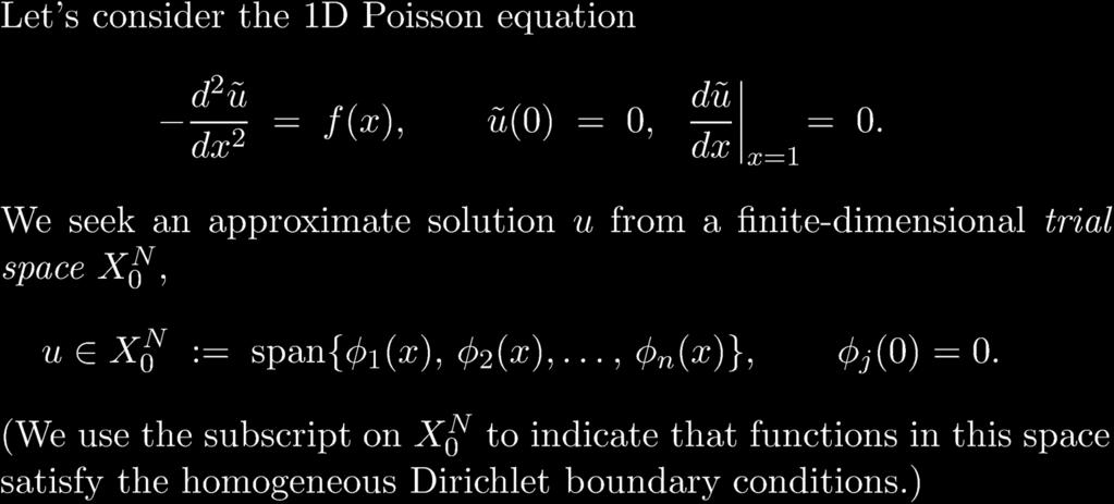
47 Weighted Residual Example: d 2 ũ = f(x), ũ(0) = ũ() = 0. dx2 Trial function (n unknowns.) nx u(x) = u j j (x) 2 X0 N : j(0) = j () = 0, j=,..., n. j= Residual (w.r.t. u): r(u) := f + d2 u dx 2 Orthogonality condition: (v, r) := Z 0 vrdx = 0 8 v 2 X N 0.

48 Orthogonality condition: (v, r) := Z 0 vrdx = 0 8 v 2 X N 0. So, for i =,...,n, v = i (n equations): ( i,r) := Z 0 i rdx = 0 = Z 0 i f + d2 u dx 2 dx. Or, Z 0 i d 2 u dx 2 dx = Z 0 i fdx.

49 An important refinement: Z 0 i d 2 u dx 2 dx = Z 0 i fdx. We can avoid requiring existence of u 00 by interpolating the expression on the left by parts: I := Z 0 {z} i v 00 d 2 u dx = {z} dx 2 du 00 Z 0 du d i dx dx dx i du dx x= x=0 = Z 0 d i dx du dx dx ( i(0) = i () = 0 for these boundary conditions). Now the test and trial functions require only the existence of a first derivative. (Admits a larger search space for approximate solutions.)

50 Inserting the expansion for du dx : Z 0 d i dx du dx dx = Z 0 d i dx nx j= u j d j dx A dx = Z 0 i(x) f(x) dx =: b i. nx j= Z d i dx dx dx d j 0 {z } =:a ij u j = b i. In matrix form: Au = b 8 >< >: a ij := b i := Z 0 Z 0 d i dx d j dx dx = (d i dx, d j dx ) =: a( i, j). i fdx = ( i,f) We refer to a( i, j) asthea inner product.

51 Example: Linear Finite Elements in D Piecewise-linear basis functions, phi i (x), i =,...,n, x 2 =[0, ]: i(x) = x x i x i x i x 2 [x i,x i ] = x i+ x x i+ x i x 2 [x i,x i+ ] = 0, otherwise. d i dx = h i x 2 [x i,x i ] = h i+ x 2 [x i,x i+ ] = 0, otherwise.

52 Sti ness matrix entries: a ij = Z 0 d i dx d j dx dx = h i h 2 i + h i+ h 2 i+ j = i, = h i h 2 i j = i, = h i+ h 2 i+ = 0, otherwise. j = i +, For uniform gridspacing h, a ij = Z 0 d i dx d j dx dx = h

53 For the right-hand side, b i = Z 0 i fdx Z i 0 j=0 j(x)f j A dx = Xn+ j=0 b ij f j dx = Bf i. B is rectangular (mass matrix): B ij := Z 0 i j dx = 3 (h i + h j ) if j = i = 6 h i if j = i = 6 h i+ if j = i +

54 If h = n+ is uniform, the n (n +2)matrix B is, B = h The system to be solved is then Au = Bf.

55 Example: d 2 ũ =, u(0) = u() = 0. dx2 Exact solution: ũ = 2 x ( x). FEM solution with n =2,h = 3, Au = h " 2 2 # u u 2! = h " # C A 0 = A. 0 " # 0

56 @ A Solving for u: u u 2 A = " 2 2 # h 2 A. Recall, " a b c d # = ad bc " d b c a # = 3 " 2 2 # So, u u 2 A = 9 3 " 2 2 # A = 9 9 A.

57 Extensions: Variable coe cients Neuman boundary conditions High-order polynomial bases Best-fit property

58 Variable Coe cients Consider k(x) > 0forx 2 := [0, ], d dx k dũ dx = f, ũ(0) = ũ() = 0. WRT: find u 2 X0 N such that Z d v dx k du dx = dx Integrate by parts a(v, u) := Set v = i (x), u = P j j(x) u j, Z Z dv dx k du dx dx = vfdx 8 v 2 X N 0. Z vfdx. Au = Bf, a ij := Becasuse k>0, A is SPD. (!) Z 0 d i dx k d j dx dx.

59 Neumann Boundary Conditions Consider k(x) > 0forx 2 := [0, ], d dx k dũ dx = f, du ũ(0) = 0, =0. dx x= Now, include u = n+(x) asavalidbasisfunction: Xn+ j= j(x)u j, v = i (x), i =,...,n+. Integration by parts Z d v dx k du dx = dx = Set v = i (x), u = P j j(x) u j, Z Z dv dx k du dx dx dv dx k du dx dx = v du Z dx x= vfdx. v du dx x=0 Au = Bf, a ij := Z Same system! ( Natural boundary conditions) A is (n +) (n +) 0 d i dx k d j dx dx.

60

61 Weighted Residual Techniques (Galerkin, FEM,...) Consider Lũ = f, plus boundary conditions (e.g., Lũ = ũ xx + cũ x ). Recall collocation with Lagrangian basis functions j(x i )= ij : u(x) := nx j=0 u j j (x) r(x) := f Lu r(x i ) := f Lu =) f(x i ) [ u xx + cu x ] xi =0 Unknown basis coe cients, u j. Residual set to zero, point-wise, at interior points x i. Other two equations come from BCs.

62 For weighted residual technique (WRT), we insist that the residual be orthogonal to a family of test functions, Find u 2 X N 0 such that Z b a v (f Lu) dx = Z b a vrdx = 0 8v 2 Y N 0 Here, X0 N := span{ j } is the space of trial functions and Y0 N := span{ i } is the space of test functions. The relationship between collocation and WRT is analogous to the relationship between least squares and interpolation. One seeks a polynomial interpolant of degree n (say) and chooses it either in a weighted (i.e., LS / WRT ) or pointwise ( interpolation / collocation ) fashion. Two common choices for Y N 0 are i = (x x i ), the Dirac delta function, or i = i, (i.e., Y N 0 = X N 0 ), termed the Galerkin method. Galerkin is far more common. Dirac delta functions yield collocation, so we see that collocation is in fact a WRT.

63 We ll focus solely on the Galerkin case. Most common bases for X N 0 are Lagrange polynomials (on good point sets) Piecewise polynomials (FEM) typically still Lagrangian

64 Questions that arise: Implementation Cost (strongly dependent on number of space dimensions) Accuracy Spectrum Other (e.g., optimality)

65

66 Trial Solution and Residual

67 Trial Solution and Residual

68 WRT and Test Functions

69 Reducing Continuity to C0

70 Weighted Residual / Variational Formulation

71 Formulation of the Discrete Problem

72 Formulation of the Discrete Problem

73 Formulation of the Discrete Problem

74 Choice of Spaces & Bases The next step is to choose the space, X 0N, and associated basis { φ i }. The former influences convergence, i.e., How large or small n must be for a given error. The latter influences implementation, i.e., details and level of complexity, and performance (time to solution, for a given error)

75 Unstable and Stable Bases within the Elements Examples of unstable bases are: Monomials (modal): φ i = x i High-order Lagrange interpolants (nodal) on uniformly-spaced points. Examples of stable bases are: Orthogonal polynomials (modal), e.g., Legendre polynomials: L k (x), or bubble functions: φ k (x) := L k+ (x) L k- (x). Lagrange (nodal) polynomials based on Gauss quadrature points (e.g., Gauss-Legendre, Gauss-Chebyshev, Gauss-Lobatto-Legendre, etc.)

76 Piecewise Polynomial Bases: Linear and Quadratic Linear case results in A being tridiagonal (b.w. = ) Q: What is matrix bandwidth for piecewise quadratic case?

77 Lagrange Polynomials: Good and Bad Point Distributions N=4 N=7 N=8 φ 2 φ 4 Uniform Gauss-Lobatto-Legendre

78 Basis functions for N=, E=5 on element 3. x 0 Ω Ω 2 Ω 3 Ω 4 Ω 5

79 Basis functions for N=, E=5 on element 3. Ω Ω 2 Ω 3 Ω 4 Ω 5 Ω Ω 2 Ω 3 Ω 4 Ω 5

80 Ω 3 basis functions for N=2, E=5 Ω Ω 2 Ω 3 Ω 4 Ω 5

81 Ω 3 basis functions for N=3, E=5 Ω Ω 2 Ω 3 Ω 4 Ω 5

82 Important Properties of the Galerkin Formulation An essential property of the Galerkin formulation for the Poisson equation is that the solution is the best fit in the approximation space, with respect to the energy norm. Specifically, we consider the bilinear form, and associated semi-norm, which is in fact a norm for all u satisfying the boundary conditions. It is straightforward to show that our Galerkin solution, u, is the closest solution to the exact ũ in the a-norm. That is, u ũ a w ũ a for all w X 0 N In fact, u is closer to ũ than the interpolant of ũ.

83 Best Fit Property, /4

84 Best Fit Property, 2/4

85 Best Fit Property, 3/4

86 Best Fit Property 4/4

87 Best Fit Viewed as a Projection

88 Best Fit Property Summary A significant advantage of the WRT over collocation is that the choice of basis for a given space, X 0N, is immaterial you will get the same answer for any basis, modulo round-off considerations, because of the best fit property. That is, the choice of Á i influences the condition number of A, but would give the same answer (in inifinite-precision arithmetic) whether one used Lagrange polynomials on uniform points, Chebyshev points, or even monomial bases. This is not the case for collocation so WRT is much more robust. Of course, Lagrange polynomials on Chebyshev or Gauss-Lobatto- Legndre points are preferred from a conditioning standpoint.

89

90 Boundary Value Problems Numerical Methods for BVPs Eigenvalue Problems Shooting Method Finite Difference Method Collocation Method Galerkin Method Standard eigenvalue problem for second-order ODE has form u 00 = f(t, u, u 0 ), a < t < b with BC u(a) =, u(b) = where we seek not only solution u but also parameter Scalar (possibly complex) is eigenvalue and solution u is corresponding eigenfunction for this two-point BVP Discretization of eigenvalue problem for ODE results in algebraic eigenvalue problem whose solution approximates that of original problem Michael T. Heath Scientific Computing 43 / 45

91 Boundary Value Problems Numerical Methods for BVPs Example: Eigenvalue Problem Shooting Method Finite Difference Method Collocation Method Galerkin Method Consider linear two-point BVP with BC u 00 = g(t)u, a < t < b u(a) =0, u(b) =0 Introduce discrete mesh points t i in interval [a, b], with mesh spacing h and use standard finite difference approximation for second derivative to obtain algebraic system y i+ 2y i + y i h 2 = g i y i, i =,...,n where y i = u(t i ) and g i = g(t i ), and from BC y 0 = u(a) =0 and y n+ = u(b) =0 Michael T. Heath Scientific Computing 44 / 45

92 Boundary Value Problems Numerical Methods for BVPs Example, continued Shooting Method Finite Difference Method Collocation Method Galerkin Method Assuming g i 6=0, divide equation i by g i for i =,...,n, to obtain linear system Ay = y where n n matrix A has tridiagonal form 2 3 2/g /g 0 0. A = /g 2 2/g 2 /g.. 2. h /g n 2/g n /g n /g n 2/g n This standard algebraic eigenvalue problem can be solved by methods discussed previously Michael T. Heath Scientific Computing 45 / 45

93