Kasetsart University Workshop. Multigrid methods: An introduction

Transcription

1 Kasetsart University Workshop Multigrid methods: An introduction Dr. Anand Pardhanani Mathematics Department Earlham College Richmond, Indiana USA A copy of these slides is available at pardhan/kaset/workshop/

2 Topics to be covered Outline of PDE solution approach Algebraic system solvers Basic iterative methods Motivation for multigrid Basic multigrid ingredients Cycling strategies Generalization to nonlinear problems Scalars a, b, c, Vectors a, b, c, Matrices A, B, C, General notation

3 PDE Solution Outline General PDE problem: Lu = f in Ω Bu = g on Ω where L = PDE operator, B = boundary operator, Ω = domain, Ω = domain boundary, and u = unknown solution Specific example: 2 u e25x = 625 x2 e 25 1 in 0 < x < 1 u(0) = 0, u(1) = 1 The analytical solution to this problem is: u(x) = e25x 1 e 25 1

4 Numerical solution method: 1. Discretize domain: Ω Ω h = Construct suitable mesh (grid) 2. Discretize PDE on Ω h : Lu = f A h u h = b h = Use finite-difference, finite-element, finite-volume... = PDE becomes algebraic system 3. Solve algebraic system for u h 4. Interpolate discrete solution u h 1-D example: 1. Grid generation (uniform spacing h with N nodes) u h Ω h 1 2 i 1 i i + 1 N 2. PDE discretization: Use finite difference At any node i, from Taylor series u i+1 = u i + hu i + h2 2 u i + h3 6 u i + h4 24 uiv i + u i 1 = u i hu i + h2 2 u i h3 6 u i + h4 24 uiv i + Add the two and get the approximation 2 u x u i 1 2u i + u i+1 2 h 2

5 Therefore, our PDE problem 2 u x = f(x) becomes u i 1 2u i + u i+1 2 h 2 Assemble over entire grid and get algebraic system where A h u h = b h f i u h = [u 1, u 2,, u i,, u N ] T b h A h = = h 2 [0, f 2, f 3,, f i,, 1/h 2 ] T and f i = 625 e25x i e Solve N N algebraic system for u h 4. Interpolate u h between nodes if necessary

6 Taylor series centered at x i for deriving other finite difference approximations Assume following uniform mesh structure: h i 4 i 3 i 2 i 1 i i + 1 i + 2 i + 3 i + 4 Taylor series expansions of function u(x) about node i u i 4 u i 3 u i 2 u i 1 u i+1 u i+2 u i+3 u i+4 = u i 4hu i + 16 h2 2 u i 64 h3 6 u i h4 24 uiv i = u i 3hu i + 9 h2 2 u i 27 h3 6 u i + 81 h4 24 uiv i = u i 2hu i + 4 h2 2 u i 8 h3 6 u i + 16 h4 24 uiv i = u i hu i + h2 2 u i h3 6 u i + h4 24 uiv i = u i + hu i + h2 2 u i + h3 6 u i + h4 24 uiv i = u i + 2hu i + 4 h2 2 u i + 8 h3 6 u i + 16 h4 24 uiv i = u i + 3hu i + 9 h2 2 u i + 27 h3 6 u i + 81 h4 24 uiv i = u i + 4hu i + 16 h2 2 u i + 64 h3 6 u i h4 24 uiv i 1024 h5 120 uv i + (1) 243 h5 120 uv i + (2) 32 h5 120 uv i + (3) h5 120 uv i + (4) + h5 120 uv i + (5) + 32 h5 120 uv i + (6) h5 120 uv i + (7) h5 120 uv i + (8)

7 Remarks: PDE transformed to system of algebraic equations With N grid points: Size of algebraic system = N N Number of unknowns = O(N) For large N, algebraic solution dominates computational effort (CPU time) Efficient algebraic solvers are very important Observe that A h is very sparse; this is typical in PDE problems Key point: Efficient algebraic solvers are crucial for solving PDE s efficiently Multigrid methods are basically very efficient algebraic system solvers

8 Linear Algebraic System Solvers Algebraic problem Au = b Given A (N N matrix) and b (N-vector), solve for u. Two main approaches: (1) Direct methods (Gauss elimination & variants) (2) Iterative methods For large, sparse, well-behaved matrices, iterative methods are much faster Multigrid methods are a special form of iterative methods We ll focus on iterative methods first

9 Basic Iterative Methods: An illustration Suppose we want to solve u 1 u 2 u 3 = Our system can be written as u 1 2u 2 + u 3 = 1 u 1 + u 2 = 2 = 2u 1 + u 2 + u 3 = 3 u 1 = 1 + 2u 2 u 3 u 2 = 2 + u 1 u 3 = 3 2u 1 u 2 Now consider the iteration scheme u k+1 1 = 1 + 2u k 2 u k 3 u k+1 2 = 2 + u k 1 u k+1 3 = 3 2u k 1 u k 2 where k denotes the iteration number Suppose the initial guess is u 0 = [0 0 0] T Then we get u 1 = [1 2 3] T u 2 = [2 3 1] T u 3 = [8 4 4] T etc. This is the classic Jacobi method If it converges, we should eventually get the exact solution

10 Iterative Methods: More general form Recap problem statement: Given A and b, solve for u Iterative procedure: 1. Pick arbitrary initial guess u 0 2. Recursively update using the formula Au = b (9) u k+1 = [I Q 1 A] u k + Q 1 b (10) where k = 0, 1, 2, is the iteration index, and Q is a matrix that depends on the specific iterative method Example: Jacobi method = Q = D Gauss-Seidel method = Q = D + L where D and L are the diagonal and lower-triangular parts of A The form (10) is useful for analysis, but in practice Q is not explicitly computed we often rewrite (10) in the form u k+1 = R u k + g (11) where R is the iteration matrix and g is a constant vector

11 Practical Implementation: Rewrite algebraic system (9) as: N a ij u j = b i, j=1 i = 1, 2,, N Split LHS into 3 parts i 1 j=1 = a ii u i = Iteration formulas: a ij u j + a ii u i + N j=i+1 i 1 b i + j=1 a ij u j = b i N j=i+1 a ij u j (12) Jacobi a ii u new i = i 1 b i + j=1 N a ij u old (13) j=i+1 j Gauss-Seidel a ii u new i = i 1 b i j=1 a ij u new j + N j=i+1 a ij u old (14) j

12 Recap of iterative procedure: 1. Pick initial guess u 0 = [u 0 1, u 0 2,, u 0 N ] 2. Recursively apply iterative formula: for k=1:k end % (Iteration loop) for i=1:n % (Loop over rows of algebraic system) end where end u k+1 i = [b i ρ = { i 1 j=1 k k + 1 a ij u ρ j N j=i+1 a ij u k j] / a ii for Jacobi for Gauss-Seidel Variants of Jacobi & Gauss-Seidel: Damped Jacobi: At each iteration k + 1, do the following: (1) Compute Jacobi iterate, say ū k+1, as before (2) Set u k+1 = ω ū k+1 + (1 ω) u k, (0 < ω 1) SOR (Successive Over-Relaxation): At each iteration k + 1, do the following: (1) Compute Gauss-Seidel iterate ū k+1 (2) Set u k+1 = ω ū k+1 + (1 ω) u k, (0 < ω < 2)

13 Convergence of Iterative Methods Depends on properties of A Assume A arises from discretizing elliptic PDE Typical behavior Fast convergence in 1st few iterations Slow convergence thereafter

14 Reason for such convergence behavior: Let initial error = e 0 e 0 can be viewed as superposition of discrete Fourier modes e 0 = e.g., w n = {cos(nπx i )} N i=1 Low n = low frequency High n = high frequency N 1 n=0 α n w n Iter. methods not equally effective on all error frequencies (1) More effective on high frequencies (HF) (see matlab animation) (2) Less effective on low frequencies (LF) Quick elimination of HF errors leads to rapid convergence initially; lingering LF errors decrease convergence thereafter

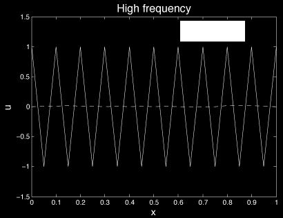
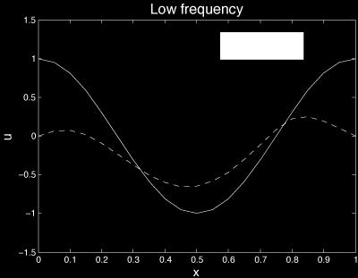
15

16 Remarks: High frequency is defined relative to N (i.e., no. of grid points) Highest visible frequency (i.e., w N 1 ) depends on N HF on coarse grid looks like LF on fine grid Example: Ω 1 N points and Ω 2 2N points Highest frequency on Ω 2 = 2 HF on Ω 1 Motivation for Multigrid Iterative methods preferentially damp HF errors This is called smoothing property Overall convergence rate is slowed by LF errors HF and LF are defined relative to grid spacing To improve convergence rate, LF must be disguised as HF This is precisely what multigrid does Multigrid = use progressively coarser grids to attenuate LF error modes

17 Convergence analysis in more detail Consider the algebraic system and the iteration algorithm Au = b u (k+1) = R u (k) + g Clearly, the exact solution u is a fixed point, since u = Ru + g u = [I Q 1 A]u + Q 1 b which is always true Subtract [u (k+1) = R u (k) + g] [u = Ru + g]. We get e (k+1) = R e (k) where e (k) is the error at the k th iterate. Let e (0) be the initial error. Then we have e (k) = R k e (0) For convergence, we want R k 0 as k From linear algebra we know that R k 0 iff ρ(r) < 1 where ρ(r) is the spectral radius (eigenvalue of largest magnitude) of R ρ(r) < 1 guarantees the method converges, and ρ(r) is the convergence rate

18 Rate of convergence Suppose we want to reduce the initial error by 1/10. Then e (M) e (0) 10 R M e (0) e (0) 10 ρ(r) M 1 10 M ln(1/10) ln(ρ(r)) M is the number of iterations needed to reduce error by 1/10 Note that ρ(r) 0 M 0 and ρ(r) 1 M Thus ρ(r) is a key indicator of the convergence rate

19 Illustration using damped Jacobi method As before, consider the PDE problem which gives the algebraic system 2 u x 2 = f(x) Au = b where A = Damped Jacobi iterations can be written as u (k+1) = R u (k) + g where R = I ωd 1 A, and D = diag(a), 0 < ω 1. The next few slides are from the the multigrid tutorial by Briggs, which contains very clear and complete visuals for this case.

20 Convergence analysis for weighted Jacobi on 1D model 1 Rω = ( 1 ω) I + ωd ( L + U ) 1 = I ωd A R ω = I ω ω λ( R ω ) = 1 λ ( A) 2 For the 1D model problem, he eigenvectors of the weighted Jacobi iteration and the eigenvectors of the matrix A are the same! The eigenvalues are related as well of 119

21 Good exercise: Find the eigenvalues & eigenvectors of A Show that the eigenvectors of A are Fourier modes! kπ jkπ λk ( A) = 4sin2, wk j = sin 2N, N of 119

22 Eigenvectors of R ω and A are the same,the eigenvalues related kπ λ k ( R ω ) = 1 2ωsin2 2N Expand the initial error in terms of the eigenvectors: e( 0 N 1 ) = ck wk k = 1 After M iterations, R M e ( N 1 N 1 M = k k k = 1 k = 1 0) c R w = c λ k M k w k The k th mode of the error is reduced by λ k at each iteration 30 of 119

23 Relaxation suppresses eigenmodes unevenly Eigenvalue Look carefully at ω = 1 N 2 k λ k kπ ( R ω ) = 1 2ωsin2 2N ω = 1/ 3 ω = 1/ 2 ω = 2/ 3 Note that if 0 ω 1 then λk( R ω) < 1 for k = 1, 2,..., N 1 For 0 ω 1, λ = 1 2ωsin2 1 2 = π N π 1 2ωsin2 h 2 = 1 ( h ) 1 O 2 31 of 119

24 Low frequencies are undamped Eigenvalue Notice that no value of ω will damp out the long (i.e., low frequency) waves. ω = 1 N 2 k ω = 1/ 3 ω = 1/ 2 ω = 2/ 3 What value of gives the best damping of the short waves? N 2 N Choose such that λ N 2 ( R ω ω ) k = ω ω = λ 2 3 N ( R ω ) 32 of 119

25 The Smoothing factor The smoothing factor is the largest absolute value among the eigenvalues in the upper half of the spectrum of the iteration matrix smoothing factor N = max λk( R ) for k N 2 For R ω, with =, the smoothing factor is, 3 since 1 N λ = λ = and < for < k < N. N 2 ω 3 2 N 2 λ k λ k N 2 But, 1 k π2 h for long waves k « of 119

26 Convergence of Jacobi on Au= Unweighted Jacobi Weighted Jacobi Wavenumber, k Wavenumber, k Jacobi method on Au=0 with N=64. Number of iterations required to reduce to e <.01 Initial guess : v kj = sin jkπ N 34 of 119

27 Weighted Jacobi Relaxation Smooths the Error Initial error: 2 v kj = sin 2j π N + 1 sin 2 16j π N + 1 sin 2 32j π N Error after 35 iteration sweeps: Many relaxation schemes have the smoothing property, where oscillatory modes of the error are eliminated effectively, but smooth modes are damped very slowly. 35 of 119

28 Multigrid Methods Main ingredients Error smoother Nested iteration Coarse Grid Correction (CGC) Multigrid notation: All quantities have subscripts to denote grid on which they are defined Error smoother Also called relaxation techniques Must efficiently eliminate oscillatory (HF) component of error Certain iterative methods are ideal Gauss-Seidel is very effective for elliptic operators Nested iteration Improve initial guess by solving on coarser grid and interpolating Can generalize to include several nested coarser grids Example: Ω 4h Ω 2h Ω h On Ω 4h : A 4h u 4h = f 4h On Ω 2h : A 2h u 2h = f 2h, use u 0 2h = I[u 4h ] On Ω h : A h u h = f h, use u 0 h = I[u 2h ]

29 Coarse Grid Correction Mechanism for attenuating LF errors Some preliminaries: We have grid Ω h and linear system A h u h = b h If u h is approximate solution, define Therefore, we have error: e h = u h u h residual: r h = b h A h u h A h u h A h u h = b h A h u h A h e h = r h (15) Note that (15) is equivalent to the original system

30 Two-grid CGC Cycle: Original grid is Ω h and linear system Introduce nested coarser grid Ω 2h Ω h CGC cycle: A h u h = b h (16) 1. Perform ν 1 smoothing iterations on (16) with some initial guess on grid Ω h ; obtain approximate solution u h. 2. Compute residual r h = b h A h u h ; restrict r h and A h to the coarse grid (Ω 2h ): A h A 2h, r h r 2h Construct the following coarse grid problem 3. Solve for e 2h. A 2h e 2h = r 2h [recall equation (15)] 4. Interpolate e 2h to fine grid & improve fine grid approximation e 2h e h u new h = u h + e h 5. Perform ν 2 smoothing iterations on (16) using u new h guess. Remarks: Step (1) is called pre-smoothing Step (5) is called post-smoothing Typical values of ν 1 and ν 2 range from 1 to 4 as initial

31 Restriction & Prolongation CGC involves inter-grid transfer operations Fine-to-coarse transfer is called restriction Coarse-to-fine transfer is called prolongation Notation: Restriction operator = I 2h h (e.g., r 2h = I 2h h [r h ]) Prolongation operator = I h 2h (e.g., u h = I h 2h[u 2h ]) Prolongation methods: Use interpolation formulas Linear interpolation is most common 1-D example u h u 2h Ω h 0 1 (2i 1) 2i (2i + 1) 2M Ω 2h 0 i 1 i i + 1 M Thus I h 2h = u 2i h u 2i+1 = u i 2h h = 1 2 (ui 2h + u i+1 2h ), (0 i M) /2 1/ /2 1/ = [2M M] matrix

32 Restriction methods Want to restrict matrix A h and vector r h from Ω h to Ω 2h I 2h h [A h ] = A 2h and I 2h h [r h ] = r 2h Can discretize original PDE on Ω 2h to get A 2h For vectors r h, we can use injection or full-weighting r h r 2h Ω h 0 1 (2i 1) 2i (2i + 1) 2M Ω 2h 0 i 1 i i + 1 M Injection: r i 2h = r 2i h Full-weighting: r i 2h = 1 4 (r2i 1 h + 2r 2i h + r 2i+1 h ) (0 < i < M) This yields the opetator I 2h h = I 2h h = OR... 1/4 1/2 1/4 1/4 1/2 1/4... = [M 2M] matrix Notice that 2I 2h h = [I h 2h] T (if we use full-weighting) = [M 2M] matrix

33 Some remarks on restriction/prolongation It is very useful to have a relation of the form I h 2h = c[i 2h h ] T (for c R) It has some important theoretical implications Furthermore, we can define A 2h = I 2h h A h I h 2h This provides an alternative way to define the coarse grid matrix, without rediscretizing the underlying PDE system. This leads to the following natural strategy for intergrid transfers 1. Define I h 2h in some suitable way 2. Define I 2h h = c[i h 2h] T (e.g., c = 1) 3. Define A 2h = I 2h h A h I h 2h These ideas apply in higher dimensions as well

34 Recall CGC cycle: Generalization to multiple grids On Ω h : A h u h = b h Ω h h On Ω 2h : A 2h e 2h = r 2h Ω 2h 2h Problem on Ω 2h has same form as that on Ω h Therefore, we can compute e 2h by introducing an even coarser grid Ω 4h, and using CGC again The problem on Ω 4h again has the same form Recursive application of CGC leads to MG cycles involving several grid levels Multigrid Cycling Strategies Obtained by using CGC recursively between multiple grid levels Common MG cycles: V -cycle, W -cycle and FMG (Full Multi- Grid)

35 V -cycle Uses one recursive CGC between pairs of grid levels Sketch of resulting grid sequence has V shape Ω h h Ω 2h 2h Ω 4h 4h Ω 8h 8h Example of four nested grid levels in 1-D. Ω h Ω 2h Ω 4h Ω 8h Grid sequence for V -cycle on 4 nested grid levels.

36 Recursive definition of V -cycle (with initial iterate v h ) v h MV h (v h, f h, ν 1, ν 2 ) It consists of the following steps: 1. If h = h c (coarsest grid), go to step 5. Else, perform ν 1 smoothing iterations on A h u h = f h with initial guess v h ; obtain v h, and assign v h v h. 2. Set r h = f h A h v h, f 2h = I 2h h r h ; define coarse grid problem A 2h u 2h = f 2h. 3. Set v 2h 0, and perform v 2h MV 2h (v 2h, f 2h, ν 1, ν 2 ) on coarse grid problem. 4. Set v h v h + I h 2hv 2h. 5. If h = h c solve A h u h = f h exactly, and set v h u h. Else, perform ν 2 smoothing iterations with initial guess v h ; obtain v h, and assign v h v h.

37 W-cycle Uses 2 recursive CGC cycles between pairs of levels Ω h Ω 2h Ω 4h Ω 8h Both V - and W -cycle are a special case of the µ-cycle. It uses µ recursive CGC cycles between pairs of levels v h MG µ h (v h, f h, ν 1, ν 2 ) 1. If h = h c (coarsest grid), go to step 5. Else, perform ν 1 smoothing iterations on A h u h = f h with initial guess v h ; obtain v h, and assign v h v h. 2. Set r h = f h A h v h, f 2h = I 2h h r h, and construct coarse grid problem A 2h u 2h = f 2h. 3. Set v 2h 0, and perform µ times: v 2h MG µ 2h (v 2h, f 2h, ν 1, ν 2 ). 4. Set v h v h + I h 2hv 2h. 5. If h = h c solve A h u h = f h exactly, and set v h u h. Else, perform ν 2 smoothing iterations with initial guess v h ; obtain v h, and assign v h v h.

38 FMG-cycle FMG stands for Full MultiGrid Generalization of the nested iteration concept Use MG cycles in place of ordinary iterations Start at coarsest level & perform nested V -, W - or µ-cycles till finest level Ω h Ω 2h Ω 4h Ω 8h

39 General form: Nonlinear PDE Problems N (u) = f B(u) = g in Ω on Ω where N is nonlinear differential operator, B is boundary operator, u is unknown, f and g are given functions Upon discretizing, we get nonlinear algebraic system: Example: N ( u) = f u xx + λe u = 0, 0 < x < 1 u(0) = u(1) = 0 Discretize on grid of spacing h u 1 = 0 u i 1 (2u i h 2 λe u i ) + u i+1 = 0, (i = 2, 3,, M 1) u M = 0 Nonlinear algebraic systems more difficult to solve than linear systems

40 Nonlinear System Solution Basic solution approaches: 1. Iterative global linearization Successive approximation Newton-type iteration 2. Nonlinear relaxation Nonlinear Jacobi, Gauss-Seidel, SOR, etc. Usual difficulties: Iterations may not converge Convergence may be very slow Initial guess affects convergence

41 Global Linearization Successive Approximation Basic idea: Iteratively lag some unknowns to linearize globally Mathematical form (drop vector notation for convenience): Original algebraic system: N(u) = f Rewrite as: A(u) u = b(u) where A and b are matrix and vector functions of u Successive approximation algorithm: 1. Pick initial guess, u 0 2. Set k = 1 3. Construct linear system: A(u k ) u k+1 = b(u k ) 4. Solve for u k+1 5. If solution is converged, stop; else, set k = k + 1 and go to step (3)

42 Global Linearization Successive Approximation Example: u xx + λe u = 0, 0 < x < 1 u(0) = u(1) = 0 Original algebraic system Rewrite as u i 1 (2u i h 2 λe u i ) + u i+1 = 0 u i 1 2u i + u i+1 = h 2 λe u i which corresponds to A = b = [0,, h 2 λe u i,, 0] T

43 Global Linearization Newton iteration Given algebraic system: N(u) = f Use Taylor series expansion about iterate u k N(u k ) + N u (uk+1 u k ) + O( u 2 ) = f Neglect higher order terms, and get Newton iteration formula N u (uk+1 u k ) = f N(u k ) Iterative solution algorithm analogous to successive approximation case Remarks Both Newton iteration and successive approximation require repeated solution of linear algebraic systems Standard linear multigrid can be used for this

44 Nonlinear Relaxation Given algebraic system: N(u) = f Rewrite as: N i (u 1, u 2,, u i,, u M ) = f i, i = 1, 2,, M Nonlinear relaxation Iteratively decouple the system Solve ith equation for u i assuming all other u s are known Jacobi variant: 1. Pick initial guess, u 0 2. Set k = 1 3. for i=1:m Solve N i (u k 1, u k 2,, u k+1 i,, u k m) = f i for u k+1 i end 4. If solution is converged, stop; else, set k = k + 1 and go to step (3)

45 Nonlinear Relaxation Remarks Can construct analogs of other linear relaxation schemes in a similar way e.g., for Gauss-Seidel, simply replace the equation in step (3) with N i (u k+1 1, u k+1 2,, u k+1,, u k m) = f i In general, step (3) involves nonlinear solution for u k+1 i ; one can use successive approximation or Newton iteration Thus, we again have inner iteration embedded within outer iteration Nonlinear relaxation schemes also often exhibit smoothing property, like their linear counterparts i

46 Nonlinear Multigrid Consider nonlinear PDE, as before N(u) = f in Ω Discretize on grid Ω h and get nonlinear algebraic system where N h is a nonlinear algebraic operator N h (u h ) = f h (17) Suppose we apply a nonlinear relaxation scheme, and get the approximate solution u h. Define Error to residual relation error: e h = u h u h residual: r h = f h N h (u h) N h (u h ) N h (u h) = r h Note that e h cannot be explicitly computed for nonlinear case However, we assume e h behaves as in the linear case quick decay of HF error modes much slower decay of LF modes

47 Nonlinear Multigrid Full Approximation Scheme (FAS) FAS is nonlinear generalization of CGC Assume nonlinear relaxation/smoothing method is available Basic steps very similar to CGC: 1. On fine grid: N h (u h ) = f h ; perform ν 1 nonlinear smoothing iterations, compute u h and r h = f h N h (u h ) 2. On 2h grid: Construct N 2h (u 2h ) = N 2h (Î2h h u h ) + I2h h r h ; solve for u 2h, and compute e 2h = u 2h Î2h h u h 3. Interpolate and correct: u new h = u h + Ih 2he 2h 4. Perform ν 2 nonlinear post-smoothing iterations Notice that step (2) computes e 2h indirectly the full solution u 2h is computed first after that we compute e 2h = u 2h Î2h h u h In linear CGC, step (2) is simpler: 2. On 2h grid: A 2h (e 2h ) = I 2h h r h ; solve for e 2h directly

48 Recap key ideas from last week Algebraic systems typically very large and sparse Efficient solvers crucial for computational efficiency Iterative solvers are attractive for such large linear systems Typical behavior of iterative methods: Fast convergence in 1st few iterations Slow convergence thereafter Reason for this: Iterative methods preferentially damp HF error modes. This is called smoothing property Overall convergence rate is slowed by LF error modes Motivation for multigrid: Take advantage of smoothing property HF and LF are defined relative to grid spacing Multigrid use smoothing on progressively coarser grids to handle LF error modes