Introduction to Algebraic and Geometric Topology Week 14

Transcription

1 Introduction to Algebraic and Geometric Topology Week 14 Domingo Toledo University of Utah Fall 2016

2 Computations in coordinates I Recall smooth surface S = {f (x, y, z) =0} R 3, I rf 6= 0 on S, I Chart (U, ) on S: I U S R 3? y V R 2 1 (u, v) =x(u, v) =(x(u, v), y(u, v), z(u, v)). I f (x(u, v), y(u, v), z(u, v)) 0. I x : V! S is a parametrization of U S.

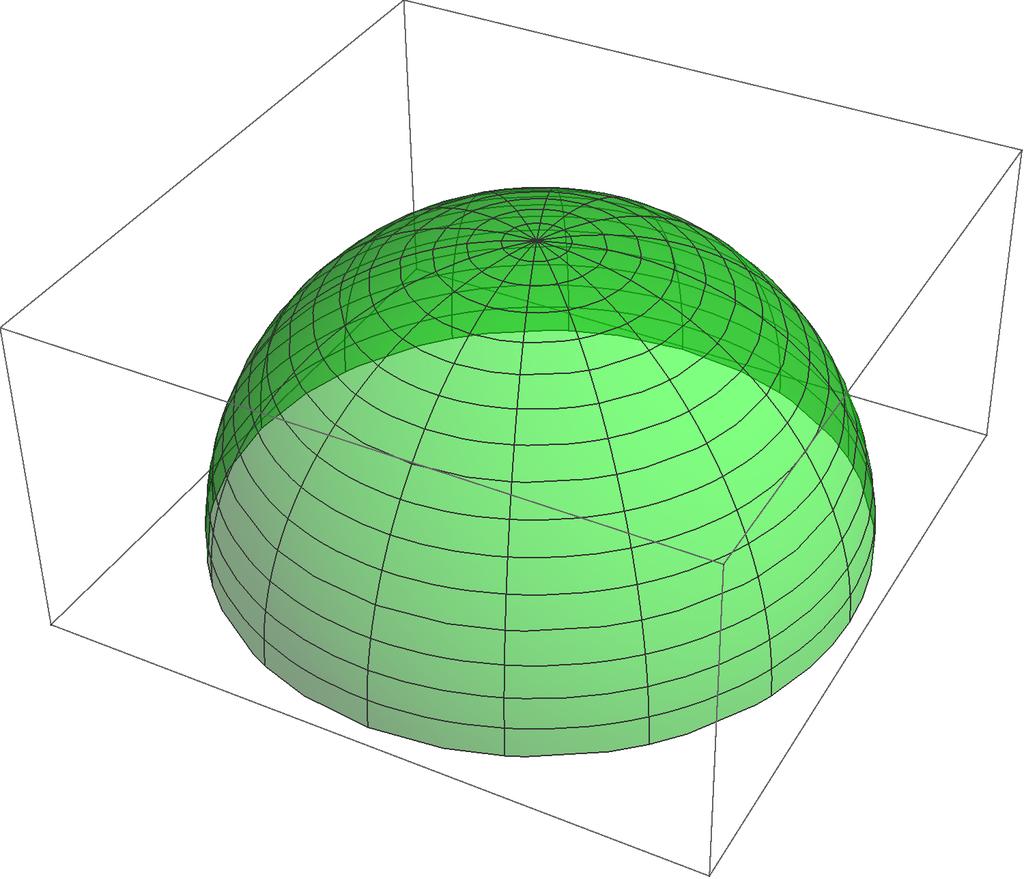
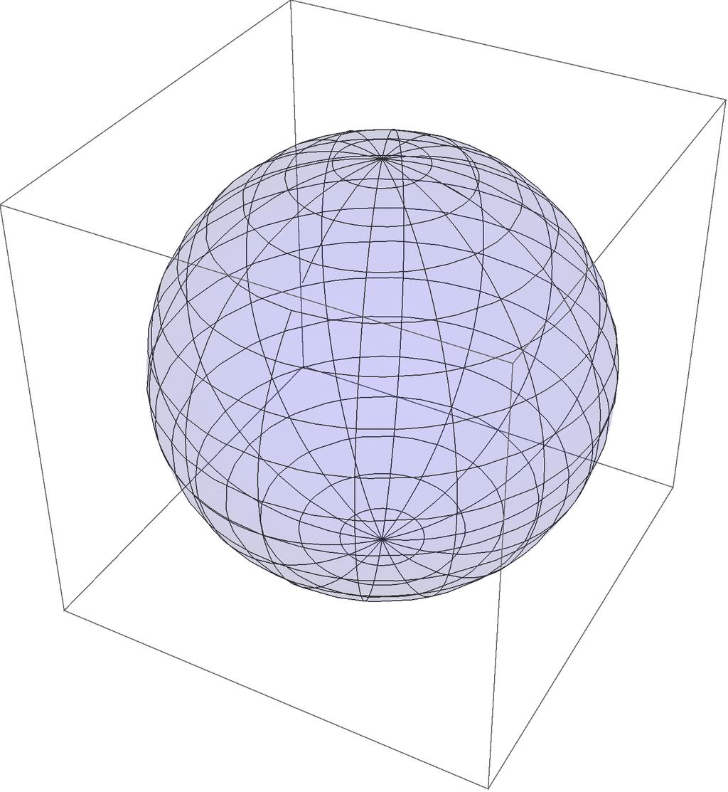
3 Example I f (x, y, z) =x 2 + y 2 + z 2 1 = 0 sphere. I U = {(x, y, z) 2 S z > 0} upper hemisphere, I V = {(u, v) 2 R 2 u 2 + v 2 < 1} unit disk in R 2. I (x, y, z) =(x, y) projection. I x(u, v) =(u, v, p 1 u 2 v 2 ). I x is a parametrization of the upper hemisphere.

4

5 I Suppose :[a, b]! S lies in coordinate chart (U, ). I Then (t) =x(u(t), v(t)) for a unique curve (u(t), v(t)) lying in V, namely (t) =(u(t), v(t)). I It is often convenient to do the calculations in terms of (u(t), v(t)). I Start with (t) =x(u(t), v(t)). I 0 (t) =x u u 0 (t)+x v v 0 (t) is its tangent vector. I 0 (t) 0 (t) is the norm squared of 0

6 I Explicitly 0 (t) 0 (t) = (x u u 0 + x v v 0 ) (x u u 0 + x v v 0 ) =(x u x u )u (x u x v )u 0 v 0 +(x v x v )v 02 I At this point it is best to forget the curve work only with the expression altogether, ds 2 =(x u x v )du 2 + 2(x u x v )dudv +(x v x v )dv 2 I What does this mean?

7 I The length of a curve is given by integrating the length of its tangent vector: L( )= Z b a ( 0 (t) 0 (t)) 1 2 dt I Could equally well be written as Z L( )= ds I What is ds?

8 I dx : T (u,v) V! T x(u,v) R 3. I If v 2 T (u,v) V, ds(v) = dx(v) =(dx(v) dx(v)) 1 2 I ds is a function of two (vector) variables,(equivalently 4 real variables): 1. a point p =(u, v) 2 V. 2. a tangent vector v =(u 0, v 0 ) 2 T p V

9 I Notation can be confusing: u, v, u 0, v 0 can mean 1. Independent variables. Then ds (u,v) (u 0.v 0 )= d p x(v) as above. 2. If evaluated on a curve (u(t), v(t)), a < t < b, then ds means the function of one variable d (u(t),v(t)) x(u 0 (t), v 0 (t)) where u 0 (t) = du dt, v 0 (t) = dv dt

10 I Going back to x : V! U S R 3, and (p, v) 2 T p V, I ds 2 is a function of p, v, quadratic in v. I d p s(v) 2 = d p x(v) 2 (usual square norm in R 3 ). I d p s 2 (v) =(x u x u )du 2 + 2(x u x v )dudv +(x v x v )dv 2, I du, dv are functions of p, v, linear in v I If v =(u 0, v 0 ), d p u(v) =u 0, d p v(v) =v 0

11 I In summary, we get ds 2 = g 11 du 2 + 2g 12 dudv + g 22 dv 2 where g 11, g 12, g 22 are smooth functions of u, v I Moreover, at every (u, v) 2 V, the matrix g11 (u, v) g G = 12 (u, v) g 21 (u, v) g 22 (u, v) is symmetric and positive definite.

12 I In fact, u 0 v 0 g11 (u, v) g 12 (u, v) g 21 (u, v) g 22 (u, v) u 0 v 0 is the same as 0 (t) 0 (t) =(x u u 0 + x v v 0 ) (x u u 0 + x v v 0 ) which is 0, and, since x u, x v are linearly independent, = 0 if and only if (u 0, v 0 )=(0, 0)

13 I Equivalent Statement g11 g 12 xu x = u g 21 g 22 x v x u x u x v x v x v I We see again that G is symmetric and positive definite.

14 I Going back to :[a, b]! U S, piecewise smooth, (t) =x(u(t), v(t)), I Recall that the length of is L( )= Z b a ds = Z b a (g 11 (u 0 ) 2 +2g 12 (u 0 v 0 )+g 22 (v 0 ) 2 ) 1 2 dt where the g ij are evaluated at (u(t), v(t)) I Usually work with the expression for ds 2 without using explictly.

15 Example Polar Coordinates: x = r cos, y = r sin. Then dx = cos dr r sin d, dy = sin dr + r cos d and ds 2 = dx 2 + dy 2 = (cos dr r sin d ) 2 +(sin dr + r cos d ) 2 which simplifies to ds 2 = dr 2 + r 2 d 2, (1)

16 Theorem Let be a curve in R 2 from the origin 0 to the circle C R of radius R centered at 0. Then 1. L( ) R. 2. Equality holds if and only if gamma is a ray = const

17

18 Proof. Let (t) =(r(t), (t), 0 apple t apple 1. Then L( )= Z 1 Z 1 (r 0 (t) 2 + r(t) 2 0 (t)) 1 2 dt r 0 (t)dt = R 0 0 and equality holds if and only if 0 (t) 0.

19 Corollary Given p, q 2 R 2, the shortest curve from p to q is the straight line segment pq.

20 Example Spherical coordinates: x = sin cos, y = sin sin, and z = cos dx = cos cos d sin sin d, dy = cos sin d + sin cos d, and dz = sin d. ds 2 = d 2 + sin 2 d 2

21

22 Theorem Let be a curve in S 2 from the north pole N to the geodesic circle = 0 of radius 0 centered at N, where 0 < 0 <. Then 1. L( ) Equality holds if and only if gamma is a great-circle arc = const

23 Proof. Let (t) =( (t), (t))0 apple t apple 1. Then L( )= Z 1 ( 0 (t) 2 + sin 2 ( (t)) 0 (t)) 1 2 dt Z (t)dt = 0 and equality holds if and only if 0 (t) 0.

24 Corollary 1. Given p, q 2 S 2, not antipodal, the shortest curve from p to q is the shorter of the two great-circle arcs from p to q 2. If p and q are antipodal, there are infinitely many curves of shortest length from p to q.

25

26 Geodesics I Temporary definition: length minimizing curves. I Examples we have seen (sphere, cylinder) suggest: locally length minimizing. I Another issue: parametrized vs. unparametrized curves. I The definition of length uses a parametrization: L( )= Z b a Z 0 (t) dt = ds

27 I But the value of L( ) is independent of the parametrization: I This means: if :[c, d]! [a, b] is an increasing function (reparametrization), Z d c Z d( ( (t)) b dt = d dt a dt dt I is an equivalence relation on curves. I Equivalence classes called unparametrized curves.

28 I L( ) depends only on the unparametrized curve I Convenient to choose a distinguished representative called parametrization by arc-length I Parameter denoted s, defined loosely as Z s = ds

29 I More precisely s(t) = Z t a d d d I s is an increasing function of t, hence invertible, inverse function t(s). I Reparametrize (t(s)), 0 apple s apple L( ) (t), a apple t apple b as I Call the reparametrized curve (t(s)) simply (s).

30 I Convention: s always means arclength. I parametrized by arclength () d ds 1. I Convention: 0 = d ds,. = d dt

31 First Variation Formula for Arc-Length I S R 3 a smooth surface (given by f = 0, rf 6= 0) I :[0, L 0 ]! S a smooth curve, parametrized by arclength, of length L 0 I endpoints P = (0) and Q = (1). I Want necessary condition for curve on S from P to Q to be shortest smooth

32 I Calculus: consider variations of, I Meaning smooth maps :[0, L 0 ] (, )! S with (s, 0) = (s) for all s 2 [0, L 0 ]. with s being arclength on (s, 0) but not necessarily on (s, t) for t 6= 0.

33 Figure: Variation with Moving Endpoints

34 I If, in addition, we have that (0, t) =P, (L 0, t) =Q for all t 2 (, ), we say that is a variation of endpoints. preserving the

35 Figure: Variation with Fixed Endpoints

36 I Necessay condition for a minimum: I Let L(t) = R L 0 d ds. 0 ds I Then dl (0) =0 for all variations of dt endpoints P, Q. with fixed I Let s compute dl (0) for arbitrary variations, then dt specialize to variations with fixed endpoints.

37 I Begin with the formula for L(t) L(t) = Z L0 0 ( s(s, t) s(s, t)) 1/2 ds I Differentiate under the integral sign dl dt = Z L ( s(s, t) s(s, t)) 1/2 (2 st (s, t) s(s, t)) ds. I Evaluate at t = 0 using that s(s, 0) s(s, 0) =1 Z dl L0 dt (0) = st (s, 0) s(s, 0) ds. 0

38 I Integrate by parts, using equality of mixed partials and the formula ( t(s, 0) s(s, 0)) s = ts (s, 0) s(s, 0)+ t(s, 0) ss (s, 0) I Get dl dt (0) =( t(s, 0) s(s, 0)) L 0 0 Z L0 0 t(s, 0) ss (s, 0) ds

39 I Define a vector field V (s) along by V (s) = t(s, 0). I This is called the variation vector field. I V (s) is the velocity vector of the curve t! (s, t) at t = 0. I V (s) tells us the velocity at which under the variation. (s) initially moves I If the variation preserves endpoints, then V (0) =0 and V (L 0 )=0,

40 Figure: Variation Vector Field

41 I We can now write the final formula dl dt (0) =V (s) 0 (s) L 0 0 Z L0 0 V (s) 00 (s) T ds. I Since V (s) is tangent to S, we replaced 00 (s) by its 00T tangential component I Necessary condition for minimizer: dl (0) =0 for all dt variations of with fixed endpoints. I equivalently Z L0 0 V (s) 00T = 0 8 V along with v(0) =V (L 0 )=0

42 I Finally this means 00T 0. I Reason: use bump functions

43 Definition Let :(a, b)! S be a smooth curve and V :(a, b)! R 3 a smooth vector field along, meaning that V is a smooth map and for all s 2 (a, b), V (s) 2 T (s) S, the tangent plane to S at (s). 1. The tangential component V 0 (s) T is called the covariant derivative of V and is denoted DV /Ds. 2. is a geodesic if and only if D 0 /Ds = 0 for all s 2 (a, b).

44 Geodesic Equation in Local Coordinates I x : V! U S R 3 as before. I The vectors x u, x v form a basis for T x(u,v) S I (s) =x(u(s), v(s)) I 0 (s) =x u u 0 + x v v 00 I Differentiate once more: 00 = x u u 00 + x v v 00 + x uu (u 0 ) 2 + 2x uv u 0 v 0 + x vv (v 0 ) 2.

45 I To find 00T, note that the first two terms are tangential I Write the sum of the last three terms as ax u + bx v + n with a, b scalar functions of u, v and n(u, v) normal. I Then (axu + bx v + n) x u (ax u + bx v + n) x v g11 g = 12 g 21 g 22 a b

46 I On the other hand, the first vector is also (xuu (u 0 ) 2 + 2x uv u 0 v 0 + x vv (v 0 ) 2 ) x u (x uu (u 0 ) 2 + 2x uv u 0 v 0 + x vv (v 0 ) 2 ) x v ) I Therefore, letting w = x uu (u 0 ) 2 + 2x uv u 0 v 0 + x vv (v 0 ) 2, w xu g11 g = 12 a w x v g 21 g 22 b I Therefore, if g 11 g 12 g 21 g 22 g11 g = 12 g 21 g 22 1

47 I We get a b g 11 g = 12 g 21 g 22 w xu w x v I Writing a b 111 u = u0 v v u u0 v v 02 I We get that the components of 00T in the basis x u, x v are u u u0 v v 02 v u u0 v v 02

48 I In particular the geodesic equation is a system of second order ODE s u u u 0 v v 02 = 0 v u u 0 v v 02 = 0 where the six coefficients i jk = i jk (u, v) are smooth functions on U, and the coefficients of u 00, v 00 are 1. I Write u = u(s) =((u(s), v(s)) for a solution of the system I Write p for a point in U and v for a vector in R 2, which we think of as a tangent vector to U at p.

49 Standard existence and uniqueness theorem for such a system of second oreder ODE s: Theorem I Given any p 0 2 U and any v 0 2 R 2 there exist 1. A nbd W of (p 0, v 0 ) in U R 2 2. An interval ( a, a) R I So that for any (p, v) 2 W there exists a unique solution u(s) of the system satisfying the initial conditions u(0) =p and u 0 (0) =v. Call this solution u(s, p, v), I It depends smoothly on the initial conditions p, v in the sense that the map u :( a, a) W! U given by (s, p, v) 7! u(s, p, v) is smooth.

50 Some Properties of the Solutions I May assume p = 0 and d 0 x is an isomtry (equivalently, (g ij (0)) = I unit matrix) I Uniqueness of solutions gives u(rs, p, v) =u(s, p, rv) for any r 2 R I Enough to consider solutions with v(0) = 1, at the expense of changing interval of existence. I or any v 0 so that v 0 = 1, there exists a neighborhood V of v 0 and an a > 0 so that the solution u(s, 0.v) exists for all (s, v) 2 ( a, a) V I Use compactness of S 1 to cover by finitely many V and take b = minimum a.

51 I Lemma There exists b 2 (0, 1] so that the solution u(s, 0, v) of the geodesic equation is defined for all (s, v) 2 ( b, b) S 1. I In other words, for any fixed length c < b all geodesics through 0 in all directions v 2 S 1 are defined up to c. I b = 1 is possible, in fact, it is the ideal situation.