Experimental Studies of Liquid Marbles and Superhydrophobic Surfaces

Transcription

1 Experimental Studies of Liquid Marbles and Superhydrophobic Surfaces Stephen James Elliott A thesis submitted in partial fulfilment of the requirements of Nottingham Trent University for the degree of Doctor of Philosophy October 2009

2 Abstract Abstract The interaction of water droplets with hydrophobic or rough, superhydrophobic solid surfaces has been studied. Such surfaces may be found in the natural world and their potential applications range from waterproof and self-cleaning surfaces to droplet microfluidics. A measure of hydrophobicity is obtained from the angle between the liquid and solid surface measured from the solid through the liquid, known as the contact angle. Variations in this angle can indicate not only a level of wetting of the surface but also small amounts of droplet movement and may be achieved by electrowetting, the application of a voltage between a liquid droplet and a substrate, and/or by varying the local topography of the surface. Photolithography and thin-film deposition fabrication techniques have been used to create hydrophobic and superhydrophobic surfaces for use in electrowetting experiments. Both AC and DC electrowetting behaviour has been investigated and the results have been shown to be in agreement with past work and well established theory. Liquid marbles have been investigated as water drops displaying extreme non-wetting behaviour, with conformal coatings forming textures similar to those formed by the topography of a super-hydrophobic surface. It has been demonstrated that for such marbles both AC and DC reversible electrowetting may be achieved and shape oscillations may be observed having nodal patterns of these oscillations which are due to stationary capillary surface waves which are accurately described by theory. Electrostatic actuation of controllable, bi-directional motion of liquid marbles has also been demonstrated on a patterned electrode structure with and without an insulating layer. Electrodeposited rough copper surfaces were created with a surface topography gradient to control the directional movement of water drops and collect them with a view to applications in large scale water harvesting. The effects of surface roughness on the sensor

3 Abstract response to liquid loading of a Quartz Crystal Microbalance (QCM) has also been investigated using three different surface coating materials. Liquid penetration between surface features differed between the materials and those upon which the liquid penetrated exhibited a characteristic low slip length or trapped mass type effect whereas those upon which it did not exhibited a slip length introduced by the air layer between the liquid and the crystal.

4 Acknowledgement There have been a number of people who have helped me throughout this project and I am eternally grateful for their input. I would particularly like to thank my supervisory team, Dr. Michael Newton, Prof. Glen McHale and Prof. Brian Pyatt for their patience, guidance and support during some difficult times and for the opportunity to be part of their highly regarded research group. I would also like to thank Mr. David Parker, Dr. Paul Roach and Dr. Neil Shirtcliffe for their wisdom and their assistance with experimentation and instrumentation. Most of all I want to thank my wife, Stella and my children Alec, Harriet and Jemima for their support and their tolerance during each and every day.

5 Contents Contents Abstract Acknowledgment Contents List of Figures List of Tables i iii iv ix xix 1. Introduction Project Overview Physical Principles Surface Tension and Wetting Dynamics Rough Surfaces and Contact Angle Hysteresis Electrowetting on Dielectric (EWOD) Summary Experimental Techniques Introduction Substrate Production Substrate Metallization Spin-Coating Dielectric Hydrophobization Superhydrophobic Substrate Electrowetting Experiments Droplet Deposition Electrical Connection 42

6 Contents Image Analysis Liquid Marbles Marble Production Marble Handling Gravitational Effects Electrowetting Experiments Contact Angle Measurement Liquid Marble Motion Control Device Production Mask Design Photolithography Electrode Connection Motion Control Experiments Liquid Marble Resonant Oscillations Substrates Image Capture Resonant Oscillation Experiments Image Processing Identification of Resonant Modes Resonance Images Profile Measurements Sources of Error Rough Copper Surfaces Electrochemical Deposition Linear Roughness Gradient Surfaces 87

7 Contents Circular Roughness Gradient Surfaces Surface Characterization Drop Mobility and Wetting Behaviour Discrete Drop Mobility Wetting Behaviour During Evaporation Wetting Behaviour During Condensation Roughness Gradient Wetting Properties Summary Electrowetting on Dielectric Introduction Experimental Method Substrate Production Electrowetting Experiments Results and Discussion Hydrophobic Surface Superhydrophobic Surface Conclusion Electrowetting of Liquid Marbles Introduction Liquid Marbles Liquid Marbles as Droplets on Superhydrophobic Surfaces Theory of Electrowetting of a Non-wetting Droplet Puddle Case Spherical Cap Case Experimental Method 146

8 Contents Marble Shape Characteristics Electrowetting Results and Discussion Marble Shape Characteristics DC Electrowetting AC Electrowetting Conclusion Resonant Oscillations of Liquid Marbles Introduction Theory of Droplet Oscillation Experimental Method Resonant Oscillation Experiments Image Processing Results and Discussion Sessile Droplets Liquid Marbles Conclusion Drop Mobility Introduction Electrostatic Liquid Marble Actuation Experimental Method Results and Discussion Superhydrophobic Gradient Surfaces Experimental Method Results and Discussion 202

9 Contents 6.4 Conclusion Conclusions and Future Developments Conclusions Future Developments and QCM Work Future Developments Superhydrophobic QCM Sensors 217 References 220 List of Publications 231

10 List of Figures List of Figures Figure 1.1 Figure 1.2 Figure 1.3 Figure 1.4 Forces acting on liquid molecules near a liquid-gas interface. A droplet in thermodynamic equilibrium on a smooth surface has an equilibrium contact angle θ e, dependent on the balance of the interfacial tensions at the three phase contact line. Contact line of a liquid drop on a solid surface advancing by a small distance, A. A gain in the solid-liquid and liquid-vapour interfaces and a loss in the solid-vapour interface results. As a droplet deposited on a solid surface spreads a) contact line advances and a dynamic contact angle, θ, ensues and b) the total surface free energy, E F, at the three phase interface changes. θ = θ e when E F = 0. Figure 1.5 A liquid drop spreads on a solid surface with a contact line edge speed, v E, proportional to the viscous dissipation. A thin precursor film advances ahead of the contact line, introducing a lubrication effect and contributing to the viscous dissipation. Figure 1.6 Figure 1.7 Figure 1.8 Figure 1.9 Figure 1.10 A droplet sitting on a rough surface in a) the non-composite case where the liquid penetrates the gaps in the surface features and makes contact with the whole of the solid surface area and b) the composite case where the liquid sits on a combination of the tops of the surface features and the air in the gaps between them. Two dimensional view of a topographically structured surface indicating the relative surface area components. Contact line of a liquid drop on a non-composite rough solid surface advancing by a small distance, A p. A gain in the solid-liquid and liquidvapour interfaces and a loss in the solid-vapour interface results. The liquid completely penetrates the surface features and maintains intimate contact with the whole of the solid surface area. Contact line of a liquid drop on a composite rough solid surface advancing by a small distance, A p shown as a) φ 1 and φ 2 as the two substrate phase fractions in contact with the liquid and b) the fraction of the surface in contact with the liquid as f s and the air gap under the drop as (1 - f s ). The liquid effectively sits upon a composite surface of the peaks of the topography and the air separating the surface features. The effects of surface roughness on contact angle for the Wenzel (blue line) and Cassie-Baxter (red line) regimes compared to a smooth surface of the same material.

11 List of Figures Figure 1.11 Figure 2.1 Figure 2.2 Two metastable energy states where the minima of one state are higher than that of the other. Transition from one state to the other requires additional energy to overcome the energy barrier that exists between the two. Vacuum chamber schematic of an Emitech K575 sputter coater. Spin speed/layer thickness calibration graph for S1813 photo-resist on an EMS 4000 spin coater. Figure 2.3 Chemical structure diagrams of a) S1813 photoresist (Shipley Co.), b) Teflon AF1600 (DuPont Polymers) 6% solution in Fluorinert FC75 (3M), c) Flutec LE15 (F2 Chemicals Ltd.), d) IC1-200 spin-on-glass (Futurrex Inc.) and e) methyltriethoxysilane (MTEOS) sol-gel foam. Structures a), c) and d) are of the main active components of the materials. Figure 2.4 Figure 2.5 Figure 2.6 Figure 2.7 Figure 2.8 Figure 2.9 Figure 2.10 Figure 2.11 Figure 2.12 Figure 2.13 An electrowetting substrate consisting of a metallized glass microscope slide with dielectric layer of thickness, d, and hydrophobic capping layer (not to scale). Electron micrograph of a metallized glass slide coated with MTEOS sol-gel foam: a) at 2kV and x500 magnification, b) at 10kV and x5000 magnification and c) vertically, in profile, at 5kV and x1000 magnification. An overhead view of the electrowetting experimental arrangement depicting the relative positions and orientation of the main components (not to scale) mounted on an optical breadboard, connection to the voltage source (in this case AC from a signal generator fed through an amplifier) and connection to the video capture PC. Electrowetting voltage for a contact angle decrease from 110 o to 75 o (solid line) and dielectric breakdown voltage (dashed line) as a function of S1813 layer thickness. The dotted line indicates the minimum S1813 layer thickness required to achieve this change in contact angle. Sample screen shot of an electrowetting drop undergoing profile fitting in the Krüss DSA-1 drop shape analysis software. Fit lines are shown in green and the automated measurements appear in the Result Window. Sol-gel basin coated in lycopodium powder. A 2µL liquid marble in silhouette illumination. The Krüss DSA-10 contact angle meter. Electrowetting configuration for a liquid marble. The hydrophobic grains provide a separation between the liquid of the marble and the substrate. Liquid marble images undergoing measurement of contact angle using ImageJ angle measuring tool showing the manually fitted baseline and tangents in a) a non-wetting state and b) a partially wetted state.

12 List of Figures Figure 2.14 Figure 2.15 Figure 2.16 Figure 2.17 Figure 2.18 Figure 2.19 Figure 2.20 Figure 2.21 Figure 2.22 Figure 2.23 Figure 2.24 Figure 2.25 Electrode pattern lithography mask with twenty electrode fingers of 0.3mm width and spacing and 1mm diameter connection pads. Flow diagram of the photolithography process for production of a patterned electrode device. Photograph of finger electrode pattern on glass slide with 0.3mm electrode width and 0.3mm spacing. Kulicke & Soffa 4522 wire bonder showing a) the whole instrument and b) a close-up of the bond head showing the capillary and N.E.F.O wand. Photograph of ball-bonded 25µm gold wire links from electrode pads to veroboard mount. Experimental arrangement for droplet actuation showing a) principle of successive application of voltage (+V, -V) sequentially across electrode fingers with respect to an upper electrode (0V) and b) schematic showing arrangement of equipment together with a top-view photograph of the substrate with electrodes and with a deposited liquid marble. Photographs showing a) switch box with twenty rotary switches, each one having positions for V +, V - and 0V applied to a single electrode and b) connections to individual finger electrodes on the device mounted in position for experiments. Configuration for inducing shape oscillations in liquid marbles by applied AC voltage. The nodal pattern around the marble surface is shown. Images of a section of a 150µL oscillating liquid marble in ImageJ with a selected area, in yellow outline, close to the apex where an anti-node is at a) peak positive and b) peak negative amplitude, the white dotted line across both images shows the peak-to-peak anti-node displacement within the selected area and c) a screen capture of a raw data z-axis profile, plotted using ImageJ, from the same 150µL liquid marble data. a) Anti-node displacement (mean greyscale value) as a function of driving frequency for the first 100Hz of the sweep for a 150µL liquid marble, the peak mean greyscale variances indicate marble resonances and b) the same data but zoomed in on the 20 50Hz region. A z-axis projection through an image stack produced from a sequence of consecutive images for one complete oscillation of a 100µL liquid drop showing the nodal pattern. The grey areas around the perimeter of the drop are the overlaid positions of anti-nodes. An image of a 100µL drop on a hydrophobic surface showing the fitted straight lines and ellipse (outlined in white) used to measure the drop perimeter.

13 List of Figures Figure 2.26 Figure 2.27 Figure 2.28 Figure 2.29 Figure 2.30 Figure 2.31 Figure 2.32 Figure 3.1 Figure 3.2 Figure 3.3 Figure 3.4 a) Electrochemical deposition arrangement for copper deposition from acidified copper sulphate solution. Three stage roughness gradient surfaces on b) a gold coated substrate and c) an aluminium substrate with three distinct areas of varying roughness. Mechanical cantilever for copper electrodeposition on circular substrates with fine control motors for substrate rotation and elevation and (inset) rubber sucker substrate mount accommodating electrical connection to the substrate surface. Photographs of circular roughness gradient surfaces from electrodeposited copper on a) gold coated slide, b) masked off copper PCB, c) rings of different roughness defined by lathe-cut grooves and d) circular cut copper PCB. The roughness levels are identifiable by a change in colour. Height profiles of electrodeposited copper on copper PCB, scans from two different areas are shown as black and grey traces. Electron micrographs at 5kV and 100x magnification of varying roughness levels, a) to g), at seven sites on the surface of a circular electrodeposited copper roughness gradient sample measured on a straight line from the near centre to the perimeter at intervals of ~3mm, h) 1000x magnification of the copper features showing a fractal type growth structure and i) 5000x magnification of the same feature showing particle composition. Apparatus for observing condensation of water vapour on a copper roughness gradient sample. Steam is directed on to the cooled sample surface where it condenses and the behaviour of the resulting droplets is captured to digital video. Overhead view of a roughness gradient sample, with a deposited water drop on the surface, positioned as for contact angle measurement using the Krüss DSA-10. The contact lines, normal to the direction of the roughness gradient, at which contact angles were measured, are shown as dashed lines. The camera aspect is parallel the gradient direction. Examples of water drops in different wetting states on a) a smooth planar untreated surface, b) a chemically hydrophobized smooth planar surface and c) a superhydrophobic rough surface. Leaves of the lotus plant showing a) drops rolling off the surface carrying dust with them and b) scanning electron micrograph of the superhydrophobic textured surface. Scanning electron micrographs at different magnifications of a) an MTEOS sol-gel and b) a patterned surface of 20µm SU-8 pillars. Schematic of the electrowetting configuration.

14 List of Figures Figure 3.5 Reversible electrowetting on a planar hydrophobic surface showing a 5µL drop with contact wire inserted and a) 0V applied bias voltage, (b) 150V DC applied bias and c) returned to 0V. Figure 3.6 Figure 3.7 Figure 3.8 Figure 3.9 Figure 3.10 Figure 3.11 Figure 3.12 Figure 3.13 Dynamic change in contact angle (θ) with voltage for a complete DC electrowetting cycle on a planar hydrophobic surface with data for the increasing voltage half of the cycle shown as ( ) and data for the decreasing half as ( ). Cosine of the contact angle (θ) as a function of the square of the applied voltage for a complete DC electrowetting cycle on a planar hydrophobic surface with data for the increasing voltage half of the cycle shown as ( ) and data for the decreasing half as ( ). Contact angle saturation is apparent at the highest voltages. Dynamic change in contact angle (θ) with RMS voltage for a complete 1kHz AC electrowetting cycle on a planar hydrophobic surface with data for the increasing voltage half of the cycle shown as ( ) and data for the decreasing half as ( ). Dynamic change in contact angle (θ) with RMS voltage for a complete 10kHz AC electrowetting cycle on a planar hydrophobic surface with data for the increasing voltage half of the cycle shown as ( ) and data for the decreasing half as ( ). Cosine of the contact angle (θ) as a function of the square of the applied RMS voltage for a complete 1kHz AC electrowetting cycle on a planar hydrophobic surface with data for the increasing voltage half of the cycle shown as ( ) and data for the decreasing half as ( ). A degree of contact angle saturation is apparent at the highest voltages. Cosine of the contact angle (θ) as a function of the square of the applied RMS voltage for a complete 10kHz AC electrowetting cycle on a planar hydrophobic surface with data for the increasing voltage half of the cycle shown as ( ) and data for the decreasing half as ( ). Contact angle saturation is again apparent at the highest voltages. The cosine of the contact angle (θ) as a function of the square of the applied RMS voltage for AC ( ) and DC ( ) electrowetting on a planar hydrophobic surface. Least squares fit lines are shown as solid for DC and dotted for AC data. Dynamic change in contact angle (θ) with RMS voltage for a complete set of 10kHz AC electrowetting cycles in 10V 5s steps on a sol-gel surface with data for the increasing voltage half of the cycle shown as ( ) and data for the decreasing half as ( ). The dashed vertical lines indicate each electrowetting sub-cycle start point.

15 List of Figures Figure 3.14 Figure 3.15 Figure 3.16 Figure 3.17 Figure 3.18 Figure 3.19 Figure 3.20 Cosine of the contact angle (θ) as a function of the square of the applied RMS voltage for a complete set of 10kHz AC electrowetting cycles in 10V 5s steps on a sol-gel surface with data for the increasing voltage half of the cycle shown as ( ) and data for the decreasing half as ( ).The dashed vertical lines indicate each electrowetting sub-cycle start point. Dynamic change in contact angle (θ) with voltage for a complete set of DC electrowetting experiments in 10V 5s steps on a sol-gel surface. The dashed vertical lines indicate each electrowetting sub-cycle start point. Cosine of the contact angle (θ) as a function of the square of the applied voltage for a complete set of DC electrowetting experiments in 10V 5s steps on a sol-gel surface. The dashed vertical lines indicate each electrowetting sub-cycle start point. Dynamic change in contact angle (θ) with RMS voltage for a Vpp 1kHz AC electrowetting cycle in 50V 5s steps on a sol-gel surface with data for the increasing voltage half of the cycle shown as ( ) and data for the decreasing half as ( ). Cosine of the contact angle (θ) as a function of the square of the applied RMS voltage for a Vpp 1kHz AC electrowetting cycle on a sol-gel surface with data for the increasing voltage half of the cycle shown as ( ) and data for the decreasing half as ( ). Dynamic change in contact angle (θ) with RMS voltage for a Vpp 10kHz AC electrowetting cycle in 50V 5s steps on a sol-gel surface with data for the increasing voltage half of the cycle shown as ( ) and data for the decreasing half as ( ). Cosine of the contact angle (θ) as a function of the square of the applied RMS voltage for a Vpp 10kHz AC electrowetting cycle on a sol-gel surface with data for the increasing voltage half of the cycle shown as ( ) and data for the decreasing half as ( ). Figure 3.21 Dynamic change in base diameter (±0.005mm) with RMS voltage for a Vpp 1kHz AC electrowetting cycle in 50V 5s steps on a sol-gel surface with data for the increasing voltage half of the cycle shown as ( ) and data for the decreasing half as ( ). Figure 3.22 Figure 4.1 Figure 4.2 Cosine of the contact angle (θ) as a function of the square of the applied voltage on a sol-gel surface for DC electrowetting ( ) and 10kHz AC electrowetting ( ) in the voltage range V RMS. Solid line and dotted line are least squares fits for the DC and AC data, respectively. A liquid marble formed by rolling a water droplet in hydrophobized lycopodium powder. Hydrophobic powder grains adhered to the liquid surface of a liquid marble.

16 List of Figures Figure 4.3 Figure 4.4 Figure 4.5 a) a droplet on super-hydrophobic micro-post surface, b) lithographic micro-posts, c) a liquid marble on a flat surface, and d) concept of a conformal skin of grains. Liquid marble puddle case with maximal radius r(z), considered as a cylinder with contact radius, r(0) and height, h. Liquid marble spherical cap case with height, h, base contact radius, r(0) and spherical cap radius, r(z). Figure 4.6 a) a spherical-cap-shaped 1µL liquid marble (R 0.7mm) and b) a 285µL marble (R 5.6mm) typical of the puddle regime. Figure 4.7 Figure 4.8 Figure 4.9 Figure 4.10 Figure 4.11 Figure 4.12 Figure 4.13 Figure 4.14 Height as a function of radius for freshly deposited water drops converted into marbles; the transition from marble to puddle with increasing volume is shown. The limiting value of puddle height gives twice the capillary length. For comparison a number of drops of 0.01M KCl solution are shown as ( ). Reversible electrowetting showing a) image of liquid marble with contact wire inserted, but no applied bias voltage; (b) image of the same marble with 100 V DC applied bias and c) image of same marble returned to 0V. Contact angle as a function of voltage for a DC electrowetting cycle with a 2µL liquid marble in 20V, 10s steps with 0-100V shown as ( ) and 100-0V shown as ( ). Contact angle as a function of voltage for a DC electrowetting cycle with a 2µL liquid drop on a lithographically patterned surface with 0-140V shown as ( ) and 140-0V shown as ( ). Contact angle as a function of voltage for a DC electrowetting cycle with a 2µL liquid marble in 10V, 1s steps with 0-100V shown as ( ) and 100-0V shown as ( ). Cosine of contact angle as a function of square of applied voltage for a DC electrowetting cycle with a 2µL liquid marble with 0-100V shown as ( ) and 100-0V shown as ( ).Solid line is a fit to Equation (4.20) with κr o = 0.1 and θ e = 174 o. Contact angle as a function of voltage for an AC electrowetting cycle with a 2µL liquid marble with 0-200V pp shown as ( ) and 200-0V pp shown as ( ). Cosine of contact angle as a function of square of applied voltage for an AC electrowetting cycle with a 2µL liquid marble with 0-200Vpp shown as ( ) and 200-0Vpp shown as ( ).Solid curve is a fit to Equation (4.20) with κr o = 0.1 and θ e = 174 o.

17 List of Figures Figure 4.15 Figure 5.1 Figure 5.2 Figure 5.3 Cosine of contact angle as a function of square of applied voltage for AC and DC electrowetting cycles with a 2µL liquid marble. For DC data 0-100V is shown as ( ) and 100-0V is shown as ( ). For AC data 0-200Vpp is shown as ( ) and 200-0Vpp is shown as ( ). Schematic illustrations of shape modes for freely oscillating spherical droplets in side-view profile. Schematic illustrations of pure oscillation modes for sessile droplets translated from images of a 100µL drop at resonance with a) immobile contact line (Noblin type I), and b) mobile contact line (Noblin type II). For type I modes the three-phase contact line corresponds to a node of the vibration, whereas for type II it is an anti-node. Configurations for inducing shape oscillations on a hydrophobic planar surface using a) a liquid marble and b) a sessile droplet. Figure 5.4 Image stack z-axis projection showing a) the first resonance of a 5µL volume liquid marble on a flat hydrophobic surface and b) a similar volume droplet in resonance. In each case two nodes are apparent on the profile above the substrate and the stacked anti-node positions appear in shades of grey. Figure 5.5 Figure 5.6 Figure 5.7 Figure 5.8 An example of anti-node displacement (mean greyscale value) as a function of driving frequency for the first 100Hz of the frequency sweep for a 100µL liquid marble. The displacement amplitude is directly proportional to the mean greyscale value within a rectangular box selection at an anti-node close to the electrode wire as a function of driving frequency. The resonant frequencies are identified by the peak variances in mean greyscale value. Anti-node displacement (mean greyscale value) as a function of driving frequency for a 50µL sessile droplet during a narrow-band sweep experiment with selection area positioned a) immediately to the right of the electrode wire, b) 50 o to the right of the wire and c) at the contact point. Anti-node displacement (mean greyscale value) as a function of driving frequency for a 100µL sessile droplet during a wide-band sweep experiment. Dashed lines are single parameter fits to the capillary wave model using γ LV = 72.8 mn m -1 and dotted lines are the equivalent fits with an adjusted value of γ LV = 64.16mN m -1. Square of frequency as a function of mode number cubed for the first five major resonances of a 10µL sessile droplet ( ) and the first eight major resonances of a 100µL sessile droplet ( ) with trendlines indicating linearity.

18 List of Figures Figure 5.9 Figure 5.10 Figure 5.11 Figure 5.12 Figure 5.13 Figure 5.14 Figure 5.15 Figure 5.16 Anti-node displacement (mean greyscale value) as a function of driving frequency for a 100µL sessile droplet during a wide-band sweep experiment. The upper and lower curves correspond to observations from the right and left hand sides of the electrode wire respectively. Dashed lines are single parameter fits to the capillary wave model using γ LV = 72.8 mn m - 1 and dotted lines are the equivalent fits with an adjusted value of γ LV = 74.66mN m -1. Anti-node displacement (mean greyscale value) as a function of driving frequency for a 10µL liquid marble during a wide-band sweep experiment. Dashed lines are single parameter fits to Equation (5.7) using γ LV = 53mN m -1 and ρ = 4550kg m -3. Solid lines are fits to the free fluid sphere model in Equation (5.1) using the same parameters. Dotted lines are the equivalent fits with an adjusted value for effective density of ρ = 1250kg m -3 and taking into account a low frequency n = 1 mode. Anti-node displacement (mean greyscale value) as a function of driving frequency for a 30µL liquid marble during a wide-band sweep experiment. Dashed lines are single parameter fits to Equation (5.7) using γ LV = 53mN m -1 and ρ = 2250kg m -3. Solid lines are fits to the free fluid sphere model in Equation (5.1) using the same parameters. Anti-node displacement (mean greyscale value) as a function of driving frequency for a 50µL liquid marble during a wide-band sweep experiment. Dashed lines are single parameter fits to Equation (5.7) using γ LV = 53mN m -1 and ρ = 1750kg m -3. Solid lines are fits to the free fluid sphere model in Equation (5.1) using the same parameters. Anti-node displacement (mean greyscale value) as a function of driving frequency for a 100µL liquid marble during a wide-band sweep experiment. Dashed lines are single parameter fits to Equation (5.7) using γ LV = 53mN m -1 and ρ = 1750kg m -3. Solid lines are fits to the free fluid sphere model in Equation (5.1) using the same parameters. Anti-node displacement (mean greyscale value) as a function of driving frequency for a 125µL liquid marble during a wide-band sweep experiment. Dashed lines are single parameter fits to Equation (5.7) using γ LV = 53mN m -1 and ρ = 1750kg m -3. Solid lines are fits to the free fluid sphere model in Equation (5.1) using the same parameters. Anti-node displacement (mean greyscale value) as a function of driving frequency for a 150µL liquid marble during a wide-band sweep experiment. Dashed lines are single parameter fits to Equation (5.7) using γ LV = 53mN m -1 and ρ = 1750kg m -3. Solid lines are fits to the free fluid sphere model in Equation (5.1) using the same parameters. Square of frequency as a function of mode number cubed for liquid marbles of volumes 10µL ( ), 30µL( ), 50µL (x), 100µL( ), 125µL (+) and 150µL ( ) with data trendlines included.

19 List of Figures Figure 5.17 Figure 5.18 Figure 5.19 Figure 6.1 Figure 6.2 Figure 6.3 Figure 6.4 Figure 6.5 Figure 6.6 Frequency as a function of mode number (log-log representation) for liquid marbles of volumes 10µL ( ), 30µL ( ), 50µL (x), 100µL ( ), 125µL (+) and 150µL ( ).For the 50µL -150µL volumes the solid lines are predictions using Equation (5.7) using the same fitting parameter value of ρ = 1750kg m -3. For the 30µL and 10µL data values of ρ = 2250kg m -3 and ρ = 4550kg m -3 have been used. Change in resonant frequency for lowest mode (n = 2) as a function of volume for liquid marbles in the range 10µL to 275µL. Change in the liquid marble resonant frequency for mode n = 2 as a function of volume (10µL to 50µL). The solid line is a prediction using Equation (5.6). A water drop on a tilted surface showing the difference between the contact angles at the leading and trailing contact lines. Liquid marbles of volume a) 1µL and b) 2µL rolling on a planar hydrophobic surface containing a finger electrode pattern upon application of a DC bias voltage sequentially to electrode pairs. Two liquid marbles of equal size (3µL) rolling together and merging upon application of a DC bias voltage sequentially to electrode pairs. Water droplets released from a vertical syringe at the edge of a superhydrophobic gradient surface roll to the least hydrophobic area at the centre and remain there. Steam condensing onto a copper superhydrophobic circular gradient surface. Evaporation of water from a copper superhydrophobic circular gradient surface. Figure 6.7 Contact angles of immobile water droplets on a copper superhydrophobic circular gradient surface at 3mm radial intervals from the centre. The four symbols represent four different radial lines at the four quadrants. Figure 6.8 Contact angle hysteresis of water droplets on a copper superhydrophobic circular gradient surface at 3mm radial intervals from the centre. The four symbols represent four different radial lines at the four quadrants.

20 List of Tables List of Tables Table 2.1 Table 2.2 Table 2.3 Table 2.4 Relevant bulk properties (where available) of S1813 photoresist (Shipley Co.) Teflon AF1600 (DuPont Polymers) 6% solution in Fluorinert FC75 (3M), Flutec LE15 (F2 Chemicals Ltd.), IC1-200 spin-on-glass (Futurrex Inc.) and methyltriethoxysilane (MTEOS) sol-gel foam. Liquid volumes used for an investigation of the gravitational effects on liquid marble shape with increasing size. Corresponding free spherical drop radii are also shown. Table 2.3 Frame rates for a given frame size and exposure of the SVSi MemView high speed CCD camera. Liquid volumes used for an investigation of the fundamental resonant frequencies of different sized liquid marbles. Corresponding free spherical drop radii are also shown. Data in bold highlight volumes used for wide band, higher resonant mode experiments.

21 Chapter 1 Introduction Chapter 1: Introduction

22 Chapter 1 Introduction 1.1 Project Overview The ability to manipulate water has been developed by many species in the natural world and is vital for their survival, whether for water collection or repellence. Some plants achieve water repellence on the surface of their leaves and use this to direct the flow of rainwater, to conserve water and as a mechanism to cleanse themselves of contaminants [1, 2]. Elsewhere, in the animal kingdom, some insects use the surface of their bodies to collect and channel water [3] or to protect fragile wing parts. Some soils are found to be naturally water repellent and this presents an ecological problem; enhanced run-off and rain splash can lead to erosion and poor water infiltration, which can create baron areas unable to sustain vegetation. It is perhaps no surprise, then, that a mechanism with such great importance in nature has many potential applications in the physical sciences. The aim of this project is to investigate control of the interaction between a liquid and a solid surface by varying the surface topography and/or the local electrostatic potential. This interaction is manifested in the form of a change in shape or movement of a liquid drop on a surface. In the ever growing world of micro electro-mechanical systems (MEMS), miniaturization is a key factor in the production of effective, efficient devices in terms of working speed, material costs and power consumption. In the case of microfluidic devices scaling down of liquid handling in fluid channels naturally leads to the manipulation of discrete liquid droplets where, for millimetre sized droplets, the hydrodynamics of the system are dominated by the effects of surface tension. A well established method for influencing the surface tension and, hence, wettability of liquids on solids at this scale is electrowetting whereby an electric potential is applied to the [conducting] liquid drop with respect to the

23 Chapter 1 Introduction underlying substrate [4-6]. This digital microfluidic technique requires minimal physical contact with the liquid drop and this makes it particularly useful in lab-on-chip type applications where discrete liquid volumes are used as micro-scale chemical or biological reactors [7]. A desirable feature of systems handling discrete drops is for the liquid to be easily transported with minimal surface adhesion and, therefore, minimal residue. Also, if the contact area is small then a greater number of smaller sites may be selected for wetting on the device. This implies that the use of superhydrophobic surfaces in conjunction with water drops would offer tuneable wetting with controllable high drop mobility and extended drop re-usability. It may also be desirable for the combination of two different liquids to occur and in this case internal mixing of the newly formed drop could be an important feature. In such applications there may be a requirement for chemical or biological processing involving solids and liquids simultaneously. In such cases it is conceivable that the mixing of the solid and liquid is undesirable or even that the liquid is used to transport the solid. It is possible that an alternative system could be used to combine these features, such as the use of liquid marbles as liquid drops with a conformable hydrophobic powder skin. It is clear that the control of liquid flow by appropriate design of the underlying surface has implications in terms of material savings and efficiency of liquid flow systems. One important ecological application of such surface designs is in the harvesting of clean water in areas where such a commodity is scarce. A relatively untapped source of water in desert areas is in the early morning mist and an appropriately designed surface could be used to capture small droplets and direct them across the surface to a collection area without any additional energy input. It is conceivable that a surface wettability gradient may be achieved by varying the surface feature height, hence the surface roughness, sampled locally by the contact line of a deposited drop. This varying roughness can produce varying

24 Chapter 1 Introduction local apparent contact angles from one side of the drop to another creating a driving force to initiate and direct motion of the drop, depending on the drop size and contact angle hysteresis [8-11]. Investigations of both the electrostatic and topographic drop manipulation have relied on the design of appropriate experiments and, primarily, the manufacture of suitable surfaces. In the case of electrostatic control this has involved the use of thin-film deposition and lithographic techniques to produce capacitive surfaces for experiments with or without direct electrical contact. For topographical control the manufacture of rough surfaces with a locally varying aspect ratio or graded height again required the use of reliable photolithography methods but also of a custom electrodeposition technique. An alternative approach to liquid drops on superhydrophobic rough surfaces is to wrap the drop in a conformal rough coating to form a liquid marble and electrostatic control of liquid marbles on planar surfaces has been investigated alongside liquid drops on superhydrophobic rough surfaces. The experimental techniques used in the project are comprehensively described in Chapter 2. One of the main problems found in electrowetting on dielectric (EWOD) with droplets on rough surfaces is that as the voltage is applied, the liquid penetrates between the surface features and does not recover upon removal of the voltage. This is a real issue in microfluidic applications as a droplet is likely to be manipulated to wet at multiple sites. In Chapter 3, well established EWOD results are re-affirmed to give a basis for comparison between hydrophobic and superhydrophobic surfaces with regard to reversibility and with reference to previous work done using lithographically patterned surfaces [12]. A new approach to electrowetting on low hysteresis surfaces is investigated in Chapter 4 with the introduction of liquid marbles as drops with a conformal superhydrophobic coating. Here the superhydrophobic surface is effectively removed from the substrate and

25 Chapter 1 Introduction wrapped around the droplets creating completely non-wetting drops which are highly mobile on any smooth solid surface. The effects of gravitational flattening of liquid marbles are shown and electrowetting characteristics are viewed with an energy minimization approach. Work with liquid marbles is extended to include an analysis of shape oscillations compared with liquid drops on a solid substrate in Chapter 5. In microfluidics droplet actuation is made easier if the liquid-solid contact area is reduced and this requires a degree of droplet levitation to achieve a spherical cap shape comparable to that of a suspended sessile drop. This may be achieved with liquid marbles where the conformal coating separates the liquid from the solid surface. Electric field driven oscillations in droplets have been shown to be controllable and have a number of applications including the ability to create selfpropelling droplets [13]. This highlights the importance of understanding oscillations in sessile drops possessing small contact areas. Resonant modes of liquid marbles and droplets are identified and described by combining the capillary-gravity wave equation with the model for oscillations in free levitated drops [14]. Reversible electrowetting in lab-on-chip applications would allow selective liquid deposition but only if the liquid drops can be moved with very little actuating force, a feature that is characteristic of liquid marbles. A method of actuating controlled motion of liquid marbles electrostatically is demonstrated in Chapter 6. The ability to manipulate droplet shape and mobility solely by locally varying the surface topography can be useful in controlling the flow rate and direction of a liquid but also in the collection of drops to form bulk liquids, as seen in nature [15]. Hence, in Chapter 6, graded height granular surfaces are created by controlled copper electrodeposition and used as devices for the control of droplet mobility by dynamically altering the contact angle. The level of mobility across these surfaces is investigated relative to surface roughness and hysteresis level.

26 Chapter 1 Introduction 1.2 Physical Principles The work in this project is based on well established theoretical principles of drops on surfaces, electrowetting and the influence of surface chemistry and/or topography. In this section the underlying basic theories that form the foundation for the work are established Surface Tension and Wetting Dynamics Evidence of surface tension phenomena can be seen all around us in ways that we often take for granted. Water can be observed balling up and rolling off the surfaces of some plant leaves like mercury droplets would on a lab bench. Some insects can walk on the surface of water, without sinking, as if it were solid. Water drops will suspend from a spiders web in beads and a metal pin can be made to float on a water surface as if on an invisible skin. These are all due to the effects of surface tension but why does it occur? If we think of the water molecules in the bulk of the liquid rather than at the surface, each molecule is subjected to intermolecular forces with its neighbours, in all directions, as shown in Figure 1.1. The average distance between molecules is such that the attractive and repulsive forces are balanced so there is no net force pulling any given molecule in any one direction. Molecules at the surface, however, experience an unbalanced force due to the relative lack of neighbouring molecules on the gas [vapour] phase side of the interface and so there is a tendency for every molecule at the surface to be pulled toward the bulk. As these molecules are equally repelled on the liquid side of the interface they remain at the surface forming the effective skin. For a volume of water in air a free spherical droplet shape is created as surface tension minimizes the surface area.

27 Chapter 1 Introduction Gas Liquid Figure 1.1 Forces acting on liquid molecules near a liquid-gas interface. If a droplet is of a size where its spherical radius, R 0, is less than the capillary length, κ -1, given by, 1 κ = γ ρg LV (1.1) (typically 2.7mm for water), where ρ is the density of the liquid and g=9.81 m s -2 is acceleration due to gravity then the effects of gravity on the drop shape are negligible. If such a drop is at thermodynamic equilibrium on a homogeneously smooth solid surface then it will adopt a spherical cap shape, as depicted in Figure 1.2. The surface tension, γ, at the liquid-gas [or vapour] interface is no longer solely responsible for the drop shape but also becomes a component at a three phase interface. From a lateral force view, at the solidliquid contact line there is a force contribution per unit length from the liquid-vapour

28 Chapter 1 Introduction interface, γ LV, the solid-liquid interface, γ SL and the solid-vapour interface, γ SV. A tangent to the resulting liquid surface profile forms a contact angle, θ, with the solid surface at the contact line. If the drop is at thermodynamic equilibrium then the sum of the force contributions is equal to zero and an equilibrium contact angle, θ e, is formed (Figure 1.2). We then have, cos θ γ γ γ = 0 (1.2) e LV + SL SV Re-arranging yields the Young equation, established by Thomas Young in 1805 [16], γ γ SV SL cos θ e = (1.3) γ LV The Young equation is generally accepted as the interfacial force balance at equilibrium although it does have limitations. It assumes that the solid surface is ideal in that it is perfectly smooth and homogeneous such that a drop deposited on the surface is immediately in an equilibrium state and one unique equilibrium contact angle exists for the system. It also does not take into account any effect on the equilibrium contact angle from the droplet size and the method of deposition. It should also be noted that direct measurement of γ SL and γ SV is not possible so the Young equation has never been experimentally verified.

29 Chapter 1 Introduction γ LV γ SV γ θ e γ SL Liquid drop Ideal solid surface Figure 1.2 A droplet in thermodynamic equilibrium on a smooth surface has an equilibrium contact angle θ e, dependent on the balance of the interfacial tensions at the three phase contact line. Another approach is to consider the surface tension components as surface energies per unit area at each interface. The interfacial free energy, E F, at the contact line is then given by, E F = A γ + A γ + A γ (1.4) SV SV SL SL LV LV If we then consider surface free energy changes if the contact line advances by a small distance, A, as shown in Figure 1.3, then part of the solid-vapour interface is replaced by a solid-liquid one causing a change in the surface free energy of (γ SL - γ SV ) A. There is also a gain in the liquid-vapour interface of γ LV cosθ (assuming any change in contact angle is a second order effect) and the total change in surface free energy, E F, corresponding to this contact line advance, is therefore, E F = ( γ ) A + γ θ A γ cos (1.5) SL SV LV Advances in the contact line occur if the droplet spreads on the surface (Figure 1.4a) and so a dynamic contact angle, θ, ensues where many different instantaneous values may be valid. The sketch of a free energy diagram in Figure 1.4b shows an example surface free energy profile for the wetting regime in Figure 1.4a. The minimum of surface free energy,

30 Chapter 1 Introduction with zero gradient, exists at local equilibrium and so this point corresponds to the equilibrium contact angle, θ e. At equilibrium E F = 0, we then have, ( γ ) + γ cos θ = 0 γ (1.6) SL SV LV e taking us back to the original Young equation (1.3). Vapour Liquid drop θ Acosθ Ideal solid surface A Figure 1.3 Contact line of a liquid drop on a solid surface advancing by a small distance, A. A gain in the solid-liquid and liquid-vapour interfaces and a loss in the solid-vapour interface results.

31 Chapter 1 Introduction a) Liquid drop θ 2 θ e θ 1 Ideal solid surface b) E F E F = 0 θ 1 θ e θ 2 θ Figure 1.4 As a droplet deposited on a solid surface spreads a) contact line advances and a dynamic contact angle, θ, ensues and b) the total surface free energy, E F, at the three phase interface changes. θ = θ e when E F = 0. On real surfaces the preferred [equilibrium] minimum energy state of a deposited drop may not be achieved at the instant the drop makes contact with the surface. Depending on the nature of the surface the drop may spread and the contact line advances as the drop attempts to achieve the equilibrium state. Spreading may also occur if there is an increase in the Laplace pressure [17] due to an increase in energy from, for example, heating or applied voltage. The Laplace pressure, P, is the pressure difference between the liquid and vapour phases due to curvature of the interface and is given by [17], 2γ LV P = (1.7) R

32 Chapter 1 Introduction where R is the spherical radius of the drop. The drop will spread until it conforms to one of two wetting regimes, depending on the solid surface; complete wetting or partial wetting and these may be distinguished by the spreading parameter, S, where, S SV ( γ γ ) = γ + (1.8) SL LV If S > 0 then the drop wets completely and θ e = 0. If S < 0 then the drop adopts the spherical cap shape where it is said to be mostly wetting if θ e 90 o and mostly non-wetting if θ e > 90 o. In this case and by combining Equation (1.8) with Equation (1.3), we obtain the Young-Dupré equation, ( cos 1) S = θ (1.9) γ LV At a molecular level, as the drop spreads it forms a film with a thickness, h, that will experience a transition from a thick liquid to an adsorbed microscopic thin layer due to surface forces in the region of the three phase contact line [18]. Disjoining pressure, Π, results from these forces and is equal to the negative derivative of the surface free energy with respect to the film thickness [19], def Π ( h) = (1.10) dh Following Derjaguin and Churaev [20], the disjoining pressure comprises a molecular (van der Waals) component, Π m, an electrostatic component, Π e, and a structural component, Π s, and may be written as, ( h) = Π ( h) + Π ( h) + Π ( h) Π (1.11) m e s

33 Chapter 1 Introduction The van der Waals and electrostatic components may be calculated using the well developed DLVO theory (Derjaguin-Landau-Verwey-Overbeek after the scientists who developed the theory) [21, 22]. If the molecules in the film and the solid substrate are more attracted than the molecules in the liquid bulk, then Π(h) > 0. A liquid film with a thickness such that dπ(h)/dh > 0 can lower its surface free energy by becoming thicker in some areas while thinning in others. This is characteristic of de-wetting and, conversely, wetting (spreading) occurs if dπ(h)/dh < 0. For very small contact angles and complete wetting, as the drop spreads Poiseuille flow (that is, flow parallel to the solid surface produced by a pressure gradient) occurs. A viscous dissipation equal to F d v E is created where v E is the edge speed (or rate of change of contact radius) of the drop and F d is the driving force, proportional to the unbalanced component of γ LV, ( cosθ cosθ ) F αγ (1.12) d LV e approximated, for small angles to, d LV 2 2 ( θ θ ) F αγ (1.13) e The dissipation is then proportional to inverse θ and v E is given by, v E LV 2 2 ( θ θ ) αγ θ (1.14) e This is the Hoffman-Tanner-deGennes law [23-25] and in the limit of a complete wetting surface, where θ e = 0, the edge speed becomes proportional to the cube of the dynamic contact angle, v E α θ 3. This expression for the dissipation does not include any effects from the thin precursor wetting film that is known to precede the advancing contact line of a spreading drop. The

34 Chapter 1 Introduction precursor film results from intermolecular long-range forces acting between molecules of the liquid and the solid substrate [19] and was first observed by Hardy in 1919 [26]. The dynamics of precursor wetting films have since been studied theoretically by, among others, Huh et al., Hervet et al., Voinov and degennes [25, 27-29] and experimentally by Léger et al., Bascom et al. and Ghiradella et al. [30-32]. In the present work the existence of a precursor film and its contribution to droplet spreading is acknowledged but the effects are not included in any of the experimental analyses. v E θ θ e Liquid drop v E Ideal solid surface Figure 1.5 A liquid drop spreads on a solid surface with a contact line edge speed, v E, proportional to the viscous dissipation. A thin precursor film advances ahead of the contact line, introducing a lubrication effect and contributing to the viscous dissipation.

35 Chapter 1 Introduction Rough Surfaces and Contact Angle Hysteresis For drops on real surfaces the notion of a single equilibrium contact angle, θ e, predicted by the Young equation (1.3) does not apply. Instead, as the drop spreads, a series of metastable energy states exist, with associated contact angles, due to the contact angle hysteresis of the surface. As a drop spreads on a homogeneously smooth surface the advancing contact line motion is continuous and smooth whereas if the surface has chemical or topographical inhomogeneities a ratcheting motion ensues. The advancing contact line becomes pinned by surface asperities which present an energy barrier. The dynamic contact angle will increase if, for example, the drop volume is increased until the energy barrier is overcome and the contact line de-pins. The maximum angle that is achieved before de-pinning occurs is called the advancing angle, θ A. If the drop is de-wetting then contact line recedes and the same pinning and de-pinning occurs. In this case the contact angle decreases, when the contact line pins, to a minimum known as the receding angle θ R. The range of possible dynamic contact angles is, therefore, prescribed by the limits θ R to θ A, where the energy barriers go to zero. Contact angle hysteresis is then defined as the difference between the advancing and receding angles, θ = θ A - θ R. Hysteresis has, therefore, been used as an indicator of surface hydrophobicity as it has been attributed to the surface roughness beneath the contact area and surface roughness contributes to the hydrophobicity. Depending on the surface topography the lowest free energy configuration is given by two generally accepted models, those of Wenzel [33] and Cassie-Baxter [34]. For the Wenzel and Cassie-Baxter regimes the underlying surface may be considered as either composite or non-composite. With a composite surface the surface area presented to the liquid drop comprises a solid fraction and an air fraction between the surface roughness

36 Chapter 1 Introduction features such that the liquid sits on a combination of the tops of the solid peaks and a cushion of air. A non-composite surface, however, consists solely of the solid surface area with no air fraction such that the liquid maintains intimate contact with the entire solid surface (Figure 1.6). Both models assume that the size of the liquid drop is very much larger than the roughness scale. a) b) Liquid drop Liquid drop Rough surface non-composite Rough surface composite Figure 1.6 A droplet sitting on a rough surface in a) the noncomposite case where the liquid penetrates the gaps in the surface features and makes contact with the whole of the solid surface area and b) the composite case where the liquid sits on a combination of the tops of the surface features and the air in the gaps between them. In the non-composite case the introduction of a surface roughness modifies the solid surface area presented to the penetrating liquid such that the ratio of actual surface area, including the non-horizontal fraction, to the geometric (horizontally projected) surface area may be termed as a dimensionless roughness factor, r 1. Consider a topographically structured surface, shown two dimensionally in Figure 1.7, with surface features of height, h. The width and spacing of the features is given by l 1 and l 2, respectively. Changes in the actual surface area, A a, and the horizontally projected surface area, A p are then given by,

37 Chapter 1 Introduction A a = h + l1 + h + l 2 and A p = l 1 + l2 and then, r A a = (1.15) A p l 1 A a h l 2 A p Figure 1.7 Two dimensional view of a topographically structured surface indicating the relative surface area components. Using an energy minimization approach, if we then consider an advance of the contact line by A p, as shown in Figure 1.8 then part of the solid-vapour interface is replaced by a solid-liquid one causing a change in the surface free energy of (γ SL - γ SV ) A a. There is also a gain in the liquid-vapour interface of γ LV cosθ and the total change in surface free energy, E F, corresponding to this contact line advance, is therefore, E F = ( SL γ SV ) Aa + γ LV θ A p γ cos (1.16) Incorporating the roughness factor, r, this becomes, E F = ( SL γ SV ) r A p + γ LV θ A p γ cos (1.17)

38 Chapter 1 Introduction At equilibrium E F = 0, we then have, w ( γ γ ) + γ cos = 0 SL SV r LV θe θ r ( γ γ ) w SV SL cos e = (1.18) γ LV This can then be substituted with the Young equation (1.3) to give, w cos θ e = r cosθ e (1.19) w where θ e and θ e are the equilibrium contact angles on the rough surface and the smooth surface, respectively. This is the well known Wenzel equation established by Wenzel in 1936 [33]. Liquid drop θ A p cosθ θ Vapour Solid A p Figure 1.8 Contact line of a liquid drop on a non-composite rough solid surface advancing by a small distance, A p. A gain in the solid-liquid and liquid-vapour interfaces and a loss in the solid-vapour interface results. The liquid completely penetrates the surface features and maintains intimate contact with the whole of the solid surface area.

39 Chapter 1 Introduction This works for non-composite surfaces while intimate contact between the solid and liquid is maintained and the liquid penetrates between the structures to give a high hysteresis surface. In practice, intimate contact is not usually maintained on high roughness surfaces unless hydrostatic pressure is applied. It is energetically favourable for the liquid to bridge the gaps between the surface features so that the drop effectively sits upon a composite surface of the peaks of the topography and the air separating the surface features. A low hysteresis state ensues and Cassie-Baxter derived a two phase equation which compensated for the differing surface chemistry [34]. If we consider the advance of the contact line by a small amount, A p, on a composite surface, as shown in Figure 1.9a there is a change in the surface free energy due to the replacement of some solid-vapour interface by solidliquid interface and in increase in the liquid-vapour interface. This time, however, there are two components for the solid-vapour/solid-liquid change, one for the solid fraction of the composite surface and one for the trapped air fraction. In this case, E F = ( γ SL γ SV ) ϕ1 Ap + ( γ SL γ SV ) ϕ2 Ap + γ LV cosθ A p (1.20) where φ 1 and φ 2 are the two substrate phase fractions in contact with the liquid, having real contact angle θ 1 and θ 2 respectively. At equilibrium E F = 0, we then have, ( γ γ ) ϕ + ( γ γ ) ϕ + γ cosθ = 0 SL cosθ SV 1 = SL SV 2 LV ( γ γ ) ( γ γ ) ϕ + ϕ c SV SL SV SL e 1 2 γ γ (1.21) LV LV Then substituting with the Young equation (1.3) gives,

40 Chapter 1 Introduction c cos θ = ϕ θ + ϕ θ (1.22) e 1 cos e1 2 cos e 2 whereθ is the observed equilibrium contact angle. c e For the case where the drop bridges the surface features the fraction of the surface in contact with the liquid can be termed f s and so the air gap under the drop is (1 - f s ) (Figure 1.9b) and we obtain, E F = ( f s ) γ LV Ap + ( γ SL γ SV ) f s Ap + γ LV cosθ A p 1 (1.23) At equilibrium E F = 0, we then have, ( 1 f ) γ + ( γ γ ) f + γ cosθ = 0 s θ LV SL SV s LV ( γ γ ) f ( 1 f ) γ c SV SL s s LV cos e = (1.24) γ LV This yields the Cassie-Baxter formula [34] when combined with the Young Equation (1.3), cosθ c e = f cosθ + (1 f ) cosθ (1.25) s e s v c where θe is the contact angle on the pattered surface, θ e is the contact angle on the flat surface andθ v is the contact angle of the drop on air. If we assume θ v to be 180 for a suspended droplet in air then Equation (1.25) becomes, c cosθ e = f s (cosθ e + 1) 1 (1.26)

41 Chapter 1 Introduction Liquid drop θ θ Vapour A p cosθ φ 1 A p Vapour A p φ 2 A p Solid Liquid drop θ θ Vapour A p cosθ f s A p Vapour A p (1-f s ) A p Solid Figure 1.9 Contact line of a liquid drop on a composite rough solid surface advancing by a small distance, A p shown as a) φ 1 and φ 2 as the two substrate phase fractions in contact with the liquid and b) the fraction of the surface in contact with the liquid as f s and the air gap under the drop as (1 - f s ). The liquid effectively sits upon a composite surface of the peaks of the topography and the air separating the surface features. Although the roughness factor, r, does not enter into the Cassie-Baxter formula, it is the balance between roughness and solid surface fraction that determines the threshold θ e at which the Cassie-Baxter state becomes more energetically favourable than the Wenzel state [35]. The addition of surface roughness serves to enhance the wetting state of a surface in the Wenzel regime, if the contact angle on a smooth surface is less than a threshold value of 90 o then roughness will further reduce it (saturating at 0 o ) and if it is greater than 90 o then it is increased (saturating at 180 o ). For the Cassie-Baxter regime,

42 Chapter 1 Introduction where the drop sits on top of the pattern, there is little effect on the contact angle on a smooth surface. This implies that the effects of any change in surface chemistry are amplified in the Wenzel state and attenuated in the Cassie-Baxter state. This is illustrated in Figure 1.10 where the expected contact angles on a rough surface of a given material (with r = 5 and f s = 0.16) are plotted against those on a smooth surface of the same material. The Wenzel state is indicated by the blue line and the Cassie-Baxter state is indicated by the red line. Attenuation Amplification Figure 1.10 The effects of surface roughness on contact angle for the Wenzel (blue line) and Cassie-Baxter (red line) regimes compared to a smooth surface of the same material.* For both these regimes the contact angle is determined by the spacing and feature shape of the surface beneath the contact line. It is the shape and spacing of the surface features beneath the whole of the contact area, however, that determines whether penetration into *Acknowledgement G. McHale

43 Chapter 1 Introduction the surface structure occurs and, hence, which regime is adopted. It is often the case that the surface structure is not simple, flat-topped and geometrically regular and the measurement of r and f s becomes extremely difficult. In such cases it is possible that neither a pure Wenzel nor pure Cassie-Baxter state occurs but, rather, a combination of both as composite and non-composite patches are presented to the liquid. These may include a secondary, smaller roughness scale existing on the primary roughness scale such that a Wenzel or Cassie-Baxter state may occur locally on the secondary roughness while the alternative state occurs on the primary roughness. This dual scale roughness requires modification of the Cassie-Baxter formula to take into account any Wenzel states and numerous studies have investigated its effects [8, 36-39]. It is also possible that, depending on the surface structure height and spacing, the Cassie- Baxter state is metastable in that a transition to the Wenzel state may occur upon increase of the hydrostatic pressure in the drop. This may arise from an increase in the Laplace pressure (Equation (1.7)), related to the drop curvature, as the drop reduces in size through evaporation. It could also be caused by compressing the drop [40], releasing it from a height so that it impacts the surface or by introducing a vibration. The meniscus formed by the drop surface between each of the surface features will penetrate further down between the structures until it makes contact with the lower solid fraction. This should not occur if the structure is sufficiently tall and/or closely packed. Jung and Bhushan stated a criterion for the meniscus to make contact with the lower solid surface based on the maximum droop of the meniscus and the depth of the cavity [41]. From a surface free energy point of view, the lowest energy state may be a Cassie-Baxter or Wenzel state depending on whether the surface is composite or non-composite. An energy barrier exists preventing the transition from one metastable state to another unless additional energy is introduced into the system, for example, vibrationally or

44 Chapter 1 Introduction electrostatically. The free energy diagram in Figure 1.11 shows the energy barrier separating two possible metastable energy states. Note that the shape of the free energy curves is purely a representation of a heterogeneous surface loosely based on the findings of Li and Neumann [42]. Johnson and Dettre [43] showed that surface roughness leads to a number of metastable states separated by energy barriers and that the energy barriers for composite surfaces are very much lower than for non-composite surfaces. More recently Patankar [38] gave an estimate of the barrier energy, G B1, for the transition of a Cassie- Baxter to Wenzel state on a periodic pillared surface (similar to Figure 1.9) as, B C ( r ) cosθ eγ LV AC G 1 = G 1 (1.27) where G C is the energy of the drop and A C is the contact area projected on the horizontal plane. E F Energy barrier E F = 0 θ e w θ e c θ Figure 1.11 Two metastable energy states where the minima of one state are higher than that of the other. Transition from one state to the other requires additional energy to overcome the energy barrier that exists between the two.

45 Chapter 1 Introduction The effects of these regimes on the mobility of drops defines whether a drop on the surface rolls off with little actuating force or remains adhered to the surface as it is tilted towards the vertical and beyond. In terms of surface classification, the two regimes have been classified by Quéré et al. as either slippy (Cassie-Baxter) or sticky (Wenzel) [36]. A measure of surface stickiness is given by the contact angle hysteresis resulting from the above metastable states and droplet roll is exhibited on low hysteresis surfaces. Studies have demonstrated that surface modifications, such as the introduction of dual roughness scales, can eliminate hysteresis, maintaining a Cassie-Baxter state [35, 39]. Johnson and Dettre provided the first thermodynamic analysis of contact angle hysteresis [43] and in a recent work by Li and Amirfazli [44] free energy formulae for the composite and non-composite systems have been derived. The traditional approach where contact angle hysteresis results from interactions at the whole of the solid liquid contact area has been adopted and quoted by much of the scientific literature. There are, however, notable exceptions to this viewpoint and some alternative approaches to hysteresis effects have emerged that focus on the importance of interactions at the contact line rather than the contact area. DeSimone et al. [45] produced a model based on the balance between released capillary energy and dissipation associated with contact line motion rather than the minimization of interfacial energies. Their model is stated as sharing some features with models associated with dry friction, fracture mechanics and elasto-plasticity, namely the requirement for a critical loading to achieve dissipation and loading rate independence. Predictions by their model are qualitatively compared to the experimental data of Dettre and Johnson [46]. In a study by Rafael Tadmor [47] interactions at the contact line on a Young type surface [16] were accommodated by including an additional term in the surface free energy of a moving contact line (Equation 1.5) such that,

46 Chapter 1 Introduction E F = ( γ ) A + γ θ A k L γ cos (1.28) SL SV LV where L is the length of the contact line and k is the energy per unit length associated with an increase, L, of the contact line. It has been noted by many studies that the Cassie-Baxter formula predicts a single value of apparent contact angle and is, therefore, unable to predict advancing and receding angles, as demonstrated experimentally by Gao and McCarthy [48]. This group has proposed that it is the movement of water molecules at any point on the contact line that contribute to hysteresis and no events occur over the contact area away from the contact line, bringing into question the relevance of the Wenzel and Cassie-Baxter theories [49]. The importance of events at the contact line has been considered by various groups through the years [43, 48, 50-52] and these have sought to modify the Cassie-Baxter theory accordingly. Several other studies have suggested that the Cassie-Baxter formula is valid if the areal fractions of the solid-liquid and liquid-vapour interfaces local to the contact line are considered. They have suggested that the local areal fractions can be quite different to the global fraction for spatially varying surface topographies and they have demonstrated that, as such, the apparent contact angle can vary significantly depending on the contact line position. Gao and McCarthy have also proposed that advancing and receding events may not be synchronous but, in fact, may be quite different processes with different activation energies [49]. In this case there may be multiple events occurring around the drop perimeter that could be microscopic advance-recede oscillations, distorting the contact line. Deviation from the Cassie-Baxter model due to contact line distortion has been considered by Drelich et al. [53] and Li et al. [54] as well as the McCarthy group [55, 56].In a recent study, Edward Bormashenko has suggested that the presence of a precursor film when wetting on

47 Chapter 1 Introduction heterogeneous surfaces may be assumed and that this may affirm the validity of the Cassie- Baxter approximation [57] Electrowetting on Dielectric (EWOD) In contrast to the enhanced wetting behaviour obtained through increased surface roughness, wetting of a smooth solid surface can be dynamically controlled by electrowetting, the application of an bias voltage, V, between a conducting drop and a counter-electrode. Electrowetting is based on the principles of electrocapillarity as first detailed by Gabriel Lippmann in 1875 [58] who formulated the Lippmann equation, eff dγ = σ dv SL (1.29) SL where eff γ SL is the effective interfacial tension, σ SL is the surface charge density and σ = CdV where C is the differential capacitance of the interface. In the so-called SL electrowetting-on-dielectric (EWOD), the solid surface upon which the liquid drop rests is a thin electrical insulator layer of thickness d coating an underlying conducting surface. Thus, a conductive droplet on the insulator creates a capacitance defined by the contact area of the droplet and the substrate. When a voltage, V, is applied between the substrate and droplet an electric charge is created and this alters the surface free energy balance. The additional energy per unit area due to the capacitance is given by ½CV 2 where for a simple planar surface the capacitance per unit area is C=ε r ε o /d, where ε o is the permittivity of free space and ε r is the dielectric constant of the insulator, and so by taking the integral of Equation (3.9) and incorporating the additional energy component we obtain,

48 Chapter 1 Introduction γ eff SL ε ε ( V ) V 2d r 0 2 = γ SL (1.30) To express in terms of a contact angle dependence on electrowetting voltage Equation (1.30) is inserted into the Young equation (1.3) and it is found that for a droplet on a flat surface the equilibrium contact angle for a given voltage is given by the basic equation for EWOD, ε rε 0 2 cosθ e ( V ) = cosθ e ( 0) + V (1.31) 2dγ LV Energetically the surface free energy from Equation (1.4) is valid at V = 0 (assuming a homogeneously smooth surface) when only surface energy exists. When a voltage is applied an electrical energy contribution, E E = ½CV 2 A SL, must be included and the total energy in the system becomes [6], E A A A 1 A 2 2 T = SVγ SV + SLγ SL + LVγ LV + SL (1.32) CV For rough surfaces, Bahadur and Garimella developed expressions for the contact angle of a drop on a microstructured surface under the influence of an electrowetting voltage in the Wenzel and Cassie-Baxter states, respectively, as [59], w ε rε 0 2 cosθ = r cos + V e θ e (1.33) 2dγ LV and c ε rε 0 2 cosθ = f 1+ cos + V 1 2 e θ e (1.34) dγ LV

49 Chapter 1 Introduction and, hence, that the transition from a Cassie-Baxter to a Wenzel state requires, ε ε 2dγ r V > cosθ e LV ( f ) ( ) r f (1.35) If an AC applied voltage is used in electrowetting then the drop shape and contact angle may follow the momentary equilibrium values at low frequencies. If the frequency exceeds the hydrodynamic response time of the drop then the response of the liquid depends only on the time average of the applied voltage and the RMS value V RMS must be used in Equation (1.31) [60]. The threshold frequency for millimetre sized drops is, typically, of the order 10 2 Hz. Upon increasing frequency, however, screening of the electric field from the interior of the drop ceases and, beyond a critical frequency, f c, a conducting drop may begin to behave as a dielectric. The critical frequency is given by [61], 2πσ l f c = (1.36) ε ε l 0 where σ l and ε l are the conductivity and dielectric constant of the liquid, respectively. The properties of the liquid, however, are of low importance compared to the properties of the insulating layers. Significant effort has been put into optimizing dielectric layers to give maximum wetting tunability while keeping the activation voltage to a minimum. To give a large tuning range the contact angle at V = 0 should be as large as possible, indicating that the dielectric material should possess hydrophobizing chemistry such as an amorphous fluoropolymer. These materials often have characteristically high dielectric strength allowing thinner layers to be used and, hence, reducing the voltage required for the onset of contact angle reduction.

50 Chapter 1 Introduction Although surface properties can dictate whether a deposited drop resides in a partial wetting, non-wetting or complete wetting state, the transition from partial to complete wetting in an electrowetting system has not been observed. This is due to the onset of contact angle saturation at higher applied voltages, found to occur at contact angles between 30 o and 80 o, depending on the system. The reasons for the contact angle saturation phenomenon are not fully understood but a number of possible causes from experimental observations have been proposed. Seyrat and Hayes have suggested that material deficiencies are responsible such that a perfectly insulating layer cannot be assumed [62]. Peykov et al. reported that saturation occurred when the surface energy of the solid-liquid interface becomes zero although it is not clear whether this applies to the effective solidliquid interface in electrowetting [63]. Trapped charges at the insulator partially screening the applied electric field was proposed by Verheijen and Prins [64] as a possible cause and Vallet et al. observed two other phenomena coinciding with the onset of saturation [65]. Firstly they noticed pulsed light emission at the contact line corresponding to current spikes in the system from discharge events that were attributed to the diverging electric field strength at the contact line. Second they observed the ejection of small satellite drops from the edge of the main drop at high voltages due to mutual repulsion of like charges at the contact line. This was, however, found to depend on the salt concentration in the liquid drop.

51 Chapter 1 Introduction 1.3 Summary The work in this project demonstrates, experimentally, the influence of superhydrophobic rough coatings on the behaviour of liquid drops in electric fields with particular focus on liquid marbles as liquid drops with a conformal superhydrophobic rough coating. A number of the behavioural properties of liquid drops are investigated including dynamic change in contact angle, shape oscillations and drop mobility. This extends to include an investigation of a wettability gradient to direct droplets to a collection area. A detailed description of the experimental techniques used in these studies is given in the following chapter.

52 Chapter 2 Experimental Techniques Chapter 2: Experimental Techniques

53 Chapter 2 Experimental Techniques 2.1 Introduction In this chapter the methods used for experimentation in the project are detailed and include the preparation of hydrophobic and superhydrophobic surfaces and substrates. The production and deposition of liquid marbles and droplets on these surfaces is described. Techniques for analysis of their behaviour during wetting, movement and oscillation under gravitational and applied electric field are then also detailed. 2.2 EWOD Electrowetting experiments performed with droplets or liquid marbles required a stable platform arranged in alignment with a video camera whose position could be adjusted. This would allow static millimetre sized drops on a fixed sample stage to be magnified and encompassed by the video image frame. Dynamic contact angle changes, as a result of the applied electric field, could then be monitored with silhouette illumination so as to give good image contrast for drop shape edge detection. Suitable substrates and an accurate method for droplet deposition were also required Substrate Production Substrates for electrowetting experiments act as the level platform for deposition, carry the grounding electrode and dielectric layer but also have a hydrophobic or superhydrophobic surface property. The substrates were fabricated using thin-film deposition techniques and

54 Chapter 2 Experimental Techniques consisted of a dielectric layer of known thickness deposited on the metallized surface of a glass slide. This would then be coated in either a hydrophobic or a superhydrophobic layer. Substrates were all produced on standard sized microscope slides (size 76.2 x 25.4 x 1mm) as these provided an adequate working area for multiple experimental sites using millimetre sized drops. With standard sized slides, there was enough of the metallized slide beyond the working area for connectivity and fixing to an experimental stage while not being too large so as to keep the experimental stage area within micrometer scale adjustment ranges Substrate metallization Substrate metallization was required to create a conducting substrate surface and clean glass slides were metallized with first titanium and then gold sputtered thin films. These were deposited in an Emitech K575 sputter coater using an Argon plasma under high vacuum with a Quartz Crystal Microbalance (QCM) measuring dynamic film thickness. A schematic of the sputtering chamber is shown in Figure 2.1. The titanium target first underwent a plasma cleaning stage before sputtering for 2mins, to a thickness of ~40nm, adequate enough to provide adhesion for the gold layer as gold will not sputter directly on to glass. No break in vacuum was required between sputtering of the titanium and gold layers and the gold layer was sputtered for 40s, to a thickness of ~100nm, on top of the titanium layer to provide a flat surface of high conductivity.

55 Chapter 2 Experimental Techniques Spin-coating dielectric Metallized slides were masked off at one end with adhesive tape, to leave a bare metal section of ~15mm for electrical connection, then washed with ethyl lactate and nitrogen blow-dried to remove any contamination. The dielectric coating used was Shipley S1813 polymer based positive photoresist spun-on using an Electronic Micro Systems 4000 spin coater. The sample was mounted on a vacuum chuck and the liquid S1813 was deposited over the whole surface from a syringe with a 0.2µm filter. The chuck was then accelerated to 500rpm for 5s and then on to the final speed for 30s to give a uniform layer. The final spin speed controls the layer thickness and Figure 2.2 shows the spin speed calibration graph for S1813 thickness (measured using a Dektak 6M stylus profilometer) on this model coating unit. This was done inside a fume cupboard within a clean room environment to reduce the risk of further contamination as any dust particles on the surface can cause inconsistent coverage by the dielectric layer. This can lead to potentially unusable areas due to likely short circuit. To further reduce this risk S1813 layers were built up by spinning on two or three thinner layers so that any pinholes were less likely to penetrate through to the underlying metal. For each layer, substrates were then positioned upside down (suspended at the edges on microscope slide spacers) over an Electronic Micro Systems precision hotplate and baked at 130 o C for 30mins to drive off the solvent and harden. Substrates were not positioned face-up on the hotplate as prior to baking the S1813 layer is very sticky and so is rather susceptible to airborne dust sticking to it. Layers of 2µm each were built up to give a total dielectric thickness, d, of 6µm for EWOD experiments using water droplets whereas for liquid marble work the dielectric layer could be thinner and 2.5µm total was used. A chemical structure diagram of the main Acknowledgement C. Evans

56 Chapter 2 Experimental Techniques components of S1813 photoresist and relevant bulk properties (where available) are shown in Figure 2.3 and Table 2.1, respectively. Gold target Titanium target Sample Vacuum chamber QCM film thickness monitor Rotating stage Figure 2.1 Vacuum chamber schematic of an Emitech K575 sputter coater Thickness/µm Spin Speed/rpm Figure 2.2 Spin speed/layer thickness calibration graph for S1813 photoresist on an EMS 4000 spin coater.

57 Chapter 2 Experimental Techniques Hydrophobization Substrates were hydrophobized by spin-coating a thin capping layer of fluoropolymer on top of the S1813 using the same EMS 4000 coater in the same environment. The masking tape was kept in place for this stage and substrates were again washed with ethyl lactate and nitrogen blow-dried prior to coating. The hydrophobizing agent used was either a solution of 30% Teflon AF1600 (DuPont Polymers) in hexaflourobenzene or undiluted Flutec LE15 (F2 Chemicals Ltd.). Chemical structure diagrams and relevant bulk properties (where available) for these two agents are shown in Figure 2.3 and Table 2.1, respectively. These were deposited on to the substrate while already spinning at a speed of 4000rpm (to give thickness ~0.5µm) as their volatile solvents evaporated very quickly and this also meant that no baking was required. Figure 2.4 shows the substrate with the spunon coatings Superhydrophobic Substrate Glass slides were metallized with sputtered titanium and gold using the Emitech K575. Under the same conditions as described in ( ), and following the same substrate cleaning procedure, a layer of IC1-200 spin-on-glass (Futurrex Inc.) was spun-on at 3000rpm for 40s using the EMS 4000 spin coater to a thickness of 0.2µm. This was then baked at 100 o C for 60s then at 200 o C for 60s on the EMS hotplate. In this case a thinner insulating layer was used to keep the required electrowetting voltage down as the superhydrophobic rough coating was much thicker than the Flutec or Teflon layer on the hydrophobic substrates. One end of the substrate was again masked off with adhesive tape

58 Chapter 2 Experimental Techniques to maintain a bare metal area for electrical connection. The superhydrophobic surface consisted of a layer of phase separated methyltriethoxysilane (MTEOS) sol-gel foam prepared, as described by Shirtcliffe et al. [66], by adding methyltriethoxysilane (MTEOS) to 0.12M HCl and 2-propanol under rapid stirring using a magnetic stirrer. This mixture was sealed and allowed to react for 60min at 22 C then 1.1M ammonia solution was added. The reagents were stirred for 1min before being deposited on to the substrates and encased by microscope slides to maintain thickness. They were then left in a sealed container for 20h to ensure that they gelled fully before the seal was broken and the samples were allowed to dry at room temperature. Compared to most sol-gels, these materials could be dried rapidly, drying over the course of a further 3 days and shrinking by 20-30%. Once dry, the samples were heated to 300 o C in a Carbolite AAF 11/3 furnace to cross-link the materials. To avoid overheating, cracking, and inconsistencies, the samples were heated at a rate of 2.5 C min -1 and held at the maximum temperature for 1h before cooling at around 5 C min -1. Chemical structure diagrams and relevant bulk properties (where available) for the spin-on-glass and the sol-gel are also shown in Figure 2.3 and Table 2.1, respectively. Electron micrographs of the coating were taken using a JEOL JSM-840A Scanning Electron Microscope and are shown in Figure 2.4. The material can be seen to be roughly consisting of aggregated particles of 2-3µm diameter (Figure 2.5a) forming structures ranging in size from around 5µm to chains up to 100µm long interspersed with gaps of similar size (Figure 2.5b). The coating thickness was found to be of the order 50µm as shown in Figure 2.5c and this justifies the much thinner insulating layer to be used simply as a precaution in case the liquid should penetrate through the gaps to the solid surface. The sol-gel is not a hardened material and was not firmly adhered to the surface so care had to be taken when handling so as not to damage it.

59 Chapter 2 Experimental Techniques a) b) c) d) e) Figure 2.3 Chemical structure diagrams of a) S1813 photoresist (Shipley Co.), b) Teflon AF1600 (DuPont Polymers) 6% solution in Fluorinert FC75 (3M), c) Flutec LE15 (F2 Chemicals Ltd.), d) IC1-200 spin-on-glass (Futurrex Inc.) and e) methyltriethoxysilane (MTEOS) sol-gel foam. Structures a), c) and d) are of the main active components of the materials. Material S1813 Teflon AF1600 (6%) Flutec LE15 IC1-200 spin-on-glass MTEOS sol-gel Density/ kg m ~600 Boiling point/ o C (solvent) (solvent) Melting point or g g -89 >600 g glass transition temp. ( g )/ o C 335 g Refractive index Dielectric @ @1MHz -- constant Breakdown field strength/ MV cm -1 Water static contact angle/ o (measured on a flat deposited layer) 10GHz 0.05@10kHz Table 2.1 Relevant bulk properties (where available) of S1813 photoresist (Shipley Co.) Teflon AF1600 (DuPont Polymers) 6% solution in Fluorinert FC75 (3M), Flutec LE15 (F2 Chemicals Ltd.), IC1-200 spin-on-glass (Futurrex Inc.) and methyltriethoxysilane (MTEOS) sol-gel foam.

60 Chapter 2 Experimental Techniques Hydrophobic layer d S1813 dielectric layer Metallized glass slide Figure 2.4 An electrowetting substrate consisting of a metallized glass microscope slide with dielectric layer of thickness, d, and hydrophobic capping layer (not to scale). a) b) c) 100µm 10µm 50µm Figure 2.5 Electron micrograph of a metallized glass slide coated with MTEOS sol-gel foam: a) at 2kV and x500 magnification, b) at 10kV and x5000 magnification and c) vertically, in profile, at 5kV and x1000 magnification.

61 Chapter 2 Experimental Techniques Electrowetting Experiments For electrowetting experiments the substrates were mounted horizontally on a height adjustable stage and held in place with crocodile clips at each end, one of which formed the electrical contact with the metal layer of the substrate. The stage was mounted in line with a CCD video camera and silhouette illumination on an optical breadboard. The breadboard was isolated from bench top vibration by rubber supports and levelled to prevent accidental roll-off of non-wetting drops. Illumination was provided by a 40W incandescent lamp behind an opaque acrylic diffuser and a glass block of thickness ~15mm to reduce heat transfer. The orientation of the stage was normal to the axis of camera view and illumination as shown in Figure Droplet deposition For the electrowetting experiments, a 0.01M KCl solution was used to aid conductivity. Droplet size was chosen to be within a range below the capillary length for water of 2.7mm where gravitational effects are less significant. These were deposited on to the substrate from a 25µL glass syringe whose scale accuracy is estimated to give drop volumes ±0.2µL. The syringe was mounted vertically in a micrometer stand giving control of needle position in x, y and z axes. The syringe needle was of 0.5mm diameter with a square-cut tip that had been hydrophobized in Flutec LE15 to aid droplet release. The needle was brought to within 20mm of the substrate surface and then the syringe plunger was depressed to give a spherical pendant drop of the required volume at the needle tip. The needle was then carefully lowered until the drop made contact with the substrate and then raised until the

62 Chapter 2 Experimental Techniques drop was released; as the drop had a much larger contact area with the hydrophobic substrate than with the needle, it preferentially remained on the substrate Electrical connection A copper contact wire of thickness ~0.1mm was brought into contact with the drop from above and a bias voltage applied as shown schematically in Figure 2.6. The contact wire was also hydrophobized in Flutec LE15 to prevent the liquid pinning to the wire. The wire was soldered to the tip of a probe to enable electrical connection to the voltage source, the other pole of which was connected to one of the crocodile clips holding the substrate in place at the bare metal end. The probe was vertically mounted on a swinging arm and this, in turn, was mounted on an x, y, z translation stage allowing full control of the electrode wire position. The use of any form of enclosure, either around just the sample stage or the whole breadboard, to allow minimization of evaporation effects by controlling humidity levels was thought, at the time, to introduce practical difficulties. The type of experimental arrangement used here required no obstruction of the electrode and droplet positioning mechanisms or the camera view. Easy access was also required to these mechanisms as well as to the sample surface, especially during liquid marble experiments as described in the following sections. Local atmospheric conditions were, as such, kept the same for all droplet types. Some effort was made, however, to increase local humidity at the sample surface by positioning two uncovered Petri dishes filled with water close to the sample stage.

63 Chapter 2 Experimental Techniques For DC voltages a Keithley 2410 source/meter was used and for AC voltages the output of an Agilent 33220A waveform generator was fed through a Trek PZD700 amplifier. In both AC and DC experiments the applied voltage was ramped up and then back down in steps to demonstrate the electrowetting reversibility of each surface. This required automated step sequences to be programmed into the voltage sources with specified step amplitude, spacing and duration. Optimum voltage ranges and sweep parameters were established in preliminary experiments to give the greatest contact angle change while maintaining drop stability; if the voltage was too low then contact angle changes were difficult to detect and if the voltage was too high, surface defects caused movement or boiling of the drop This meant that applied voltages were kept to a minimum to avoid short circuit via pinholes in the dielectric substrate coating and to keep below the breakdown voltage of the dielectric. The voltage, V, required to give a desired change in contact angle, cosθ, for a given thickness, d, of dielectric layer can be obtained from the electrowetting equation and is given by, 2dγ LV cosθ V ( cosθ ) = (1.31) ε ε r 0 where γ LV = 72.8 mn m -1 is the surface tension of water at 20 o C in air, ε r is the relative permittivity (or dielectric constant) of the dielectric layer and ε 0 = 8.85 F m -1 is the permittivity of free space. In practice the actual value for γ LV would be different to the accepted value for water as the ambient temperature of the lab was measured to be 23 o C (the value for water reduces to 72.0 mn m -1 at 25 o C) and the 0.01M KCl solution has values of mn m -1 and mn m -1 at 20 o C and 25 o C respectively. The electrowetting relationship is shown graphically for a contact angle decrease from 110 o to 75 o on S1813 as the solid line in Figure 2.7 [60] where the critical voltage for dielectric

64 Chapter 2 Experimental Techniques breakdown, in this case 30V µm -1, is also shown by the dashed line. The point of intersection between these two lines indicates the minimum thickness required, at this dielectric strength on S1813, to achieve this cosθ. Despite great care being taken during substrate production a number of pinholes did exist on the hydrophobic substrates causing punchthrough quite often, each time rendering a site useless on the substrate surface and reducing its useable area. Acknowledgement G. Wells

65 Chapter 2 Experimental Techniques PC with video capture board Micrometer syringe Light source Video camera b) 1000 Hz Sample stage Voltage source Electrode Figure 2.6 An overhead view of the electrowetting experimental arrangement depicting the relative positions and orientation of the main components (not to scale) mounted on an optical breadboard, connection to the voltage source (in this case AC from a signal generator fed through an amplifier) and connection to the video capture PC. V/Volts S1813 thickness/µ m Figure 2.7 Electrowetting voltage for a contact angle decrease from 110 o to 75 o (solid line) and dielectric breakdown voltage (dashed line) as a function of S1813 layer thickness. The dotted line indicates the minimum S1813 layer thickness required to achieve this change in contact angle.

66 Chapter 2 Experimental Techniques Image capture and analysis The profile of the drop was captured in silhouette illumination using a Genie DN8706 CCD video camera, with a 2x magnification microscope objective lens of focal length 50mm attached, connected to a PC via an IDS Falcon video capture board. The camera was mounted on an x, y, z micrometer stage to allow full positional control. The images were captured and analysed using Krüss DSA-1 drop shape analysis software. For electrowetting experiments a video sequence was captured to encompass the ramped voltage cycle. The DSA software uses one of five methods to evaluate the properties of the drop and the user may select the fitting method that best suits the contact points for a given drop shape and surface type. Particularly suited to dynamic contact angle measurements, Tangent 1 and Tangent 2 methods determine the contact angle from the slope of a function at the contact point, to which the drop profile is fitted only in the region of the baseline, but require good image quality with no protrusions. For static, symmetrical drops the Height/width method calculates contact angles from height-width relationship of a rectangle enclosing the drop profile, considered as being a segment of a circle. This method is more suited to smaller drops, as is the similar Circle fitting method except this method copes more easily with protrusions. Sessile drop fitting can only be used for static, symmetrical drops with no protrusions but is claimed to be, theoretically, the most accurate. This method incorporates a profile correction, to allow for the effects of the liquid weight. Each shape-fitting algorithm relies on identification of the drop edge in contrast with the background, hence the requirement for silhouette illumination. To determine the drop shape the software calculates the root of the second derivative of the brightness levels so as to identify the points of greatest change in brightness. This gives a tangential intersection with a baseline, corresponding to the substrate surface, that is user defined and positioned or

67 Chapter 2 Experimental Techniques automatically generated. Once a best-fit method is established the software measures specified parameters frame-by-frame for an entire captured video sequence and tabulates the results. This automated routine was particularly useful for sequences captured in electrowetting experiments where the applied voltage was ramped up and down as the whole sequence may last for in excess of 120s and, with a frame rate of 25-30fps, manual measurement would be very time consuming. A sample screen shot of a drop undergoing profile fitting is shown in Figure 2.8 where the fit lines are shown in green on the drop image. The consistency of the fits was checked visually during the automated process and any anomalies could be easily identified within the Result Window whereupon those data were disregarded. Once certain parameters are entered into the software, such as ambient temperature and the syringe needle diameter as a reference measurement, the software calculates a magnification factor to accurately scale the image. Then parameters such as drop base diameter, drop max. diameter, drop height and contact angles (left, right, mean) could be measured and recorded. Tangent 1 and Tangent 2 methods were found to be the only ones that would fit to drops on superhydrophobic sol-gel substrates and so these two methods were used for the flat, hydrophobic surfaces too for consistency.

68 Chapter 2 Experimental Techniques Figure 2.8 Sample screen shot of an electrowetting drop undergoing profile fitting in the Krüss DSA-1 drop shape analysis software. Profile fit lines are shown in green and the automated measurements appear in the Result Window.

69 Chapter 2 Experimental Techniques 2.3 Liquid Marbles As an alternative to drops on superhydrophobic surfaces, drops encased in a conformal superhydrophobic surface were investigated. The conformal coating in this case took the form of silane treated yellow spores of the moss Lycopodium. Such drops are termed liquid marbles [67-72] and exhibit certain properties more akin to solid spheres than liquid drops such as very high mobility and robust shape. The effect of gravity on their shape was investigated as well as their mobility and wetting behaviour upon application of a bias voltage. This required development of techniques for consistently creating and handling liquid marbles of varying sizes, while keeping as close to a monolayer coating of powder grains as possible Marble Production The main problem to overcome when creating liquid marbles is the liquid drop becoming pinned to the surface before it has chance to be completely coated in hydrophobic powder grains. If this happens then it is difficult to get the drop moving again and even then there is a likelihood of some liquid separating from the main drop to remain pinned to the surface. If the underlying surface is a superhydrophobic one then it becomes easier to keep the drop moving until it is completely powder coated and a liquid marble is fully formed. If the surface is dished then it also becomes easier to contain the marble as its mobility increases, so a superhydrophobic MTEOS sol-gel foam [66] was cast in the shape of a watch glass to act as a suitable marble carrier. This was achieved by first forming the solgel in a circular, straight-sided mould of diameter 70mm and depth ~10mm giving a flat

70 Chapter 2 Experimental Techniques top surface but a concave underside due to shrinkage during the synthesis. A similar, but of slightly smaller diameter mould was then pressed into the sol-gel like a pastry cutter to remove a circular portion. This portion was then turned over so that the concave surface became the new top surface giving a shallow, basin shape. Lycopodium powder, with grains of size d g = (17±3)µm, were hydrophobized by immersing in cyclohexane with added hexamethyldisilizane for 48h and then dried in a vacuum oven at 40 o C. The powder was then dispersed thinly but evenly over the surface of the sol-gel basin (Figure 2.9) by sprinkling it with the powder then agitating it while tilting in all directions. This ensured that the powder grains evenly dusted as much of the basin surface as possible, becoming trapped by the porous nature of the sol-gel. Agitation helped to minimize the build-up of grains in any one area and the excess was then allowed to be shaken off. Droplets of 0.01M KCl solution were deposited from a 25µL syringe (or a 200µL micro-pipette for larger marbles) onto the powder and as the droplets were made to roll around the powder coated them transforming them into highly mobile liquid marbles (Figure 2.10). Although the amount of powder available to the rolling droplet was reduced by removing as much excess as possible, this provided one of only two control measures for the amount of powder adsorption on the surface. The other was to closely observe the developing marble so that as soon as complete mobility and total powder coverage were achieved the marble was removed from the powder (usually after 1-3 circular orbits, depending on drop size). These methods are crude but for the most part marbles appeared to have a coating consisting of individual grains with water visible between them in places, particularly for the larger sizes. Surface concentration of powder grains is difficult to quantify but from visual assessment of silhouette images the surface coverage is estimated to be in the region 80-90%. Achieving a powder monolayer was most difficult with the smallest marble volumes (<10µL) as the orbital rolling action exposed all sizes to the same

71 Chapter 2 Experimental Techniques amount of powder. In these cases a measurement of the roughness scale on the silhouetted marble profiles indicated a build up of no more than two powder grains (based on d g = (17±3) µm). These grains provide the conformal coating and ensure the water within the marble does not come into direct contact with any substrate upon which the marble rests. They also contribute to the separation, d, between the conducting metal surface and the liquid and so a factor of 2 increase in this contribution will affect the capacitance of the system c= sε r ε o /d, where ε o and ε r are the permittivity of free space and relative permittivity, respectively. Although the value of ε r for lycopodium powder is unavailable the effect of a build up of grains on the dielectric properties of the marble thus tends toward the assumption of a solid powder surface rather than a composite powder-air surface.

72 Chapter 2 Experimental Techniques Figure 2.9 Sol-gel basin coated in lycopodium powder. Figure 2.10 A 2µL liquid marble in silhouette illumination.

73 Chapter 2 Experimental Techniques Marble handling Once a liquid marble had been produced it was transferred to the sample stage and positioned for experimentation while remaining intact, free from contamination and within a short enough time to avoid evaporation effects. Depending on the size of the marble, liquid evaporates from between the powder grains after a period of time until the drop shape is diminished. The powder coating remains as a husk which collapses in on itself, starting at the top of the marble. Water containers positioned close to the sample stage were also employed here to increase the local humidity and help minimize evaporation (see ). Actual evaporation rates were not measured as the use of images could only offer changes in radius or height as indicators and these could not be measured reliably due to masking by the powder coating. Rates could, however, have been established from change in mass and compared to those for liquid drops. Nonetheless, for a marble of typical size for electrowetting experiments containing 2µL of liquid, evaporation effects meant that the experiment duration could not exceed three minutes so a reliable method for fast transfer was vital. This was less of an issue with larger marbles as the volume of liquid becomes larger compared to the surface area exposed to air so liquid loss by evaporation takes much longer to affect the drop shape. However, although liquid marbles are robust compared to liquid drops, the larger the marble the more likely it is that the powder coating will split, due to the mass of the liquid, allowing liquid to leak out and the marble to collapse. It was, therefore, important that the marbles were not made to roll too fast or over obstacles or allowed to fall and impact on a surface. The method used involved allowing the marble to roll into the dished end of a metal laboratory spatula which was then used to carry it to the sample stage. The edge of the spatula was kept close up to the edge of the sol-gel basin so there was no gap or step for

74 Chapter 2 Experimental Techniques the marble to overcome. This was then tilted to allow the marble to roll out on to the substrate surface and a small section of plastic was used as a barrier to prevent the marble rolling off; this could also then be used to manoeuvre the marble into position on the surface. The edge on one side of the spatula was filed to a sharp taper so that it would meet the surface without imposing a step for the marble to roll off, allowing a smooth transition on to the surface. After each experiment, used marbles which remained mobile were removed using a light current of air and any that had collapsed or burst were removed by blotting with paper towel. Any powder debris was removed using a small artists paint brush Gravitational effects To investigate the shape changes of liquid marbles due to gravity as their size increases, measurements of height and diameter were taken for marbles ranging from 0.5µL to 300µL. The actual volume sequence used is given in Table 2.2. Distilled water was used for the liquid drop as there was no requirement for improved conductivity but a representative selection of the volume range were repeated using 0.01M KCl solution to confirm that the data was valid for the salt solution as well. The profile of the marble was captured in silhouette illumination using the DSA-1 drop shape analysis software on a Krüss DSA-10 contact angle meter (Figure 2.11). The camera on this system has manual focus adjustment and zoom adjustment up to 4.5x which meant that it could accommodate the largest marble size in its image frame while still creating a large enough image of the smallest sized marble for measurements to be taken. The zoom level was kept constant for as many consecutive sizes as possible, however, so as to reduce the amount of image re-

75 Chapter 2 Experimental Techniques calibration required; each time the zoom level changes a new magnification factor in pixels/mm has to be calculated to correctly scale the image and the system does this using an image of a syringe needle of known diameter. The DSA-10 camera is a fixed part of the system with only tilt adjustment as it relies on the stage being movable. It is mounted at one end of a linear optical bench with the light source for silhouette illumination mounted at the opposite end. Between the two is the sample stage which is adjustable in all three axes. An automatic dosing syringe holder is mounted over the sample stage and this allows variable speed liquid dispensing controlled from within the DSA-1 software. The syringe mount may be tilted upwards to allow refilling or, in this case, to be out of the way of marble transfer onto the sample stage. Each liquid marble was created and transferred to a glass slide on the sample stage, using the techniques described in the previous two sections, whereupon an image was captured and the magnification factor noted. Images for all marble sizes were captured before any measurements were taken. Then, the manual Line Draw tool in the image processing software ImageJ v1.41 (NIH) [73] was used to determine the marble maximum diameter and height measured from the slide surface. The DSA-1 software is capable of determining drop height and diameter but in practice, for the liquid marbles, it was found that the level of granular roughness made it very difficult for the DSA-1 software to fit to the drop and hence perform accurate measurements.

76 Chapter 2 Experimental Techniques V/µL R/mm V/µL R/mm V/µL R/mm V/µL R/mm Table 2.2 Liquid volumes used for an investigation of the gravitational effects on liquid marble shape with increasing size. Corresponding free spherical drop radii are also shown.

77 Chapter 2 Experimental Techniques Electrowetting Experiments The experimental arrangement described in (2.2.2) was used again here along with the hydrophobic substrate described in ( ) except this time the drop was in the form of a liquid marble. The micrometer mount syringe was also removed from the breadboard as drops were not being deposited directly from the syringe on to the substrate. A lower volume drop of 2µL was used to ensure as close to perfect spherical shape as possible and hence the highest Young angle, θ e. This provided the closest analogy to a superhydrophobic surface while being large enough for an experiment to be conducted before the liquid evaporated. The electrowetting schematic is shown in Figure 2.12 where a representation of the powder grains separating the drop from the surface is also shown. As the marble can be thought of as a drop with a superhydrophobic surface wrapped around it the arrangement of powder grains, which does not follow any geometric pattern, is comparable to the sol-gel superhydrophobic surface described in ( ). Although the powder forms an insulating layer it was necessary to use the hydrophobized and insulated substrate to prevent short circuit should the liquid penetrate between the grains. The marble surface, during production, can gather more than a monolayer of grains and the excess grains are left as a trail when the marble first rolls on a flat surface. During positioning of the marble on the electrowetting substrate a degree of roll is unavoidable and the resulting trail has the effect of debris on the surface when taking measurements. This effect was minimized by encouraging the marble to roll further, hence losing most of the excess grains and ensuring the captured image was as free from obstruction as possible. This exercise also confirmed that the marble had not burst upon deposition and was mobile prior to electrowetting. Wetting behaviour was again characterized by measurement of the dynamic contact angle.

78 Chapter 2 Experimental Techniques Contact angle measurement With the liquid marbles the DSA-1 software could not identify the contact points due to the roughness of the surface coupled with the fact that the marble was effectively a completely non-wetting drop with contact angle approaching 180 o. This made it impossible for the software to fit the marble profile and perform dynamic contact angle measurements. In this case the measurements were made on single frames using the angle measurement tool in the ImageJ [73] image processing software following enhancement of the image brightness and contrast. This method requires a baseline to be drawn manually (by cursor drag) at the solid surface and a second line to be drawn tangentially to the marble surface at the solid-marble interface. The software then measures the angle between these two lines. Examples of manually fitted baseline and tangent are shown in Figure 2.13 with a) non-wetting and b) partially wetting liquid marbles. The manual placement of a baseline and tangents is, in itself, a source of error but each angle was measured six times and a mean value taken to minimize measurement errors. For images taken from video sequences an image was chosen from the centre of a sample window. This window would encompass all frames captured between changes in applied voltage and hence a modal average image was used. For manual measurements a scaling factor was calculated from the image of a known size simulated drop in the form of a steel ball-bearing where the measured diameter in pixels was related to the measured diameter in millimetres.

79 Chapter 2 Experimental Techniques Sample stage Syringe mount Camera Light source Figure 2.11 The Krüss DSA-10 contact angle meter. Hydrophobic grains 0.01M KCl solution AC or DC bias voltage Insulator layer Metal contact Substrate Figure 2.12 Electrowetting configuration for a liquid marble. The hydrophobic grains provide a separation between the liquid of the marble and the substrate.

80 Chapter 2 Experimental Techniques Figure 2.13 Liquid marble images undergoing measurement of contact angle using ImageJ angle measuring tool showing the manually fitted baseline and tangents in a) a non-wetting state and b) a partially wetted state.

81 Chapter 2 Experimental Techniques 2.4 Liquid Marble Motion Control In a separate sequence of experiments focusing on actuating controlled droplet motion a new substrate type was designed and fabricated. This contained an electrode pattern to which a bias voltage could be sequentially applied to each electrode beneath a liquid marble. A system for sequentially switching the applied voltage between electrodes was established along with a method of connectivity with the small scale electrode pattern Device Production The basic electrowetting substrate described in ( ) was essentially being produced again here but with the metallized surface electrode taking the form of a parallel finger configuration using photolithographic techniques. The second or ground electrode was then either an opposite polarity neighbouring electrode or a separate flat plate electrode suspended closely above the marble. This differed from the penetrating wire electrode used in electrowetting as such a method would not allow the marble to move Mask Design A parallel finger electrode arrangement was designed using Altium DXP PCB design software and laser printed on to transparent acetate to create a photolithography mask (Figure 2.14). The mask was printed as the monochromic negative of the design so that the electrodes appeared as gaps in an otherwise totally black area large enough to cover a

82 Chapter 2 Experimental Techniques standard microscope slide. The pattern was designed to give twenty electrode fingers of width 0.3mm with 0.3mm spacing, a ratio giving at least one electrode and space beneath a 1µL (diameter ~1.2mm) or 2µL marble (diameter ~1.6mm) while still being large enough to be fabricated with this crude type of mask. To allow connectivity one end of each electrode finger was extended at 90 o and terminated with a circular pad of diameter 1mm Photolithography The photolithography process for the production of a patterned electrode device is shown by the flow diagram, Figure A glass slide was spin-coated with a 1.5µm layer of S1813 photoresist using an EMS 4000 spin coater (as described in ( )) and then preexposure baked face down on an EMS hotplate at 100 o C for 75s to drive off the solvent. This stage is essential for the photo-sensitivity of the resist layer although overbaking will degrade the layer by either reducing the solubility or destroying the sensitizer. The slide was then placed resist-side-down on to a UV light box (RS Components), with the electrode pattern mask sandwiched between the two, and exposed to UV light for 75s. This was found to be the optimum exposure time to give good feature definition without removing electrodes by over-exposure. The slide was then immediately immersed in a 50% solution of Shipley Microposit developer in 18MΩ cm -1 de-ionized water and agitated for <10s until fully developed; developing removes the portion of photo-resist that has been exposed to UV light. Following nitrogen blow-dry the slide was metallized with sputtered titanium to a thickness of ~40nm followed by gold to a thickness of ~100nm using an Emitech K575 sputter coater (as described in ( )) and then placed face up in an acetone bath for a lift-off stage for >40mins. This stage removes all the remaining photo-

83 Chapter 2 Experimental Techniques resist and the metal film that coats the resist, leaving the metal coating on glass in the desired electrode pattern as shown in Figure The device was not coated with an insulating layer so as to allow a lower applied voltage, reduce charge accumulation and because only 50% of the substrate beneath the marble would be conducting anyway. However, it was found that the ejection of some powder grains from the charged marble surface could lead to gaps in the coating. The liquid could then penetrate between the grains to contact the substrate surface where a short circuit between electrodes would occur. As such, in later experiments devices coated with an insulating S1813 layer of thickness 1.3µm, and a thin coating of Flutec LE15, were used. Figure 2.14 Electrode pattern lithography mask with twenty electrode fingers of 0.3mm width and spacing and 1mm diameter connection pads.

84 Chapter 2 Experimental Techniques Glass slide Spin coat photoresist Expose through acetate mask Develop pattern in photoresist Sputter coat with Ti/Au Lift off to give final metal electrode pattern Figure 2.15 Flow diagram of the photolithography process for production of a patterned electrode device. Figure 2.16 Photograph of finger electrode pattern on glass slide with 0.3mm electrode width and 0.3mm spacing.

85 Chapter 2 Experimental Techniques Electrical Connection Electrical connections to the electrodes were by flying leads terminated with 4mm plugs but it was not possible to solder leads directly to the small contact pads as the heat from a soldering iron caused the metal pad to be removed from the slide. Instead the device was adhered to a copper-clad Veroboard to which the leads could be soldered. To connect the electrode pads to the Veroboard a Kulicke & Soffa 4522 ball bonder (Figure 2.17 a)) was used to create gold wire links. The ball bonder comprises a bonding head that feeds thin gold wire (in this case 25µm) vertically through a ceramic capillary (Figure 2.17 b)) positioned above a heated work holder. The work holder was kept at the factory optimised temperature of 85 o C. Close to the capillary tip is a metal wand connected to a negative voltage generator forming the Negative Electronic Flame Off (N.E.F.O) system used to create the bonding ball; a spark is generated between the wire and the wand and this terminates the wire with a gold ball whose size may be controlled. The bond head descends to a preset search height to allow final positioning of the work piece and then the ball is bonded to the substrate by a combination of physical down-force by the head and ultrasonic vibration through the capillary for a specified time. The bond head then returns to the search height creating a wire loop bonded to the substrate at one end. The other end of this loop is then moved to the second bond site and the bond process is repeated. The bond time, force and ultrasonic power may be adjusted by the user to suit the wire thickness and substrate material in use. These parameters may differ between first and second bonds. An electronically controlled wire clamp on the bonding head allows the loop to be formed and performs the tear and tail operation. This breaks the wire feed from the second bond and leaves enough wire protruding from the capillary tip for the next ball. A

86 Chapter 2 Experimental Techniques stereo microscope provides a magnified view of the local work area which facilitates final positioning and optimization of the search height and bond parameters. Figure 2.18 shows the finger electrode substrate bonded to underlying Veroboard with gold wire links ballbonded to the electrode pads. Microscope Bond head Heated stage a) a) N.E.F.O wand b) Capillary Figure 2.17 Kulicke & Soffa 4522 wire bonder showing a) the whole instrument and b) a close-up of the bond head showing the capillary and N.E.F.O wand. Figure 2.18 Photograph of ball-bonded 25µm gold wire links from electrode pads to veroboard mount.

87 Chapter 2 Experimental Techniques Motion Control Experiments Experiments were conducted using virtually the same breadboard set-up that was used in the marble electrowetting experiments (as described in 2.3.4), with the camera, stage and illumination similarly aligned, but with some modifications. The positioning of the veroboard-mounted device on the sample stage left no space to accommodate the glass block used for heat shielding so the incandescent light source was replaced with a fluorescent one to reduce heating. The probe-mounted electrode wire positioned above the sample stage was replaced with a section of copper plate of thickness ~0.5mm, width ~3mm and length ~20mm. The plate was soldered to the probe tip but then bent through 90 o to give a flat, horizontal electrode. This was positioned above the marble acting as the reference electrode and fixed at 0V. Figure 2.19 shows a) the principle of operation of sequentially applying a voltage (V +, V - ) to a series of electrodes beneath a liquid marble with respect to an upper electrode at 0V and b) schematically, the experimental arrangement with an inset photograph of the finger electrode device with the upper electrode offset to reveal a deposited liquid marble. There was no longer a requirement for electrical connection to the substrate via the crocodile clip which clamped it to the sample stage as each electrode was individually connected to one of twenty rotary switches housed in a purpose built switch box. Each switch was interconnected to be multi-position such that each electrode could be switched to and from any combination of V +, V - or 0V. The photographs in Figure 2.20 show a) the switch box with twenty rotary switches, each one having positions for V +, V - and 0V applied to a single electrode and b) connections to individual finger electrodes on the device mounted in position for experiments. A DC bias of 150V was connected to the switch box across two series resistors of 10 MΩ with a centre tap-off providing the reference voltage.

88 Chapter 2 Experimental Techniques Liquid marbles were created and transferred to the device as described in (2.3.1) and (2.3.2) one or two at a time and then the upper electrode was swung into position above the marble but not in contact with it. The +75V and -75V relative to the upper electrode were applied sequentially to adjacent electrodes under the marble and the Krüss DSA-1 software was used to capture a video sequence of the resulting change in marble position. In later experiments patterned electrode devices of the same configuration were spin-coated with an S1813 insulating layer which meant higher DC voltages of 200V 400V could be used. In these experiments the voltage was applied with reference to neighbouring electrodes removing the need for a separate plate above the marble.

89 Chapter 2 Experimental Techniques a) b) Figure 2.19 Experimental arrangement for droplet actuation showing a) principle of successive application of voltage (+V, -V) sequentially across electrode fingers with respect to an upper electrode (0V) and b) schematic showing arrangement of equipment together with a top-view photograph of the substrate with electrodes and with a deposited liquid marble. a) b) Figure 2.20 Photographs showing a) switch box with twenty rotary switches, each one having positions for V +, V - and 0V applied to a single electrode and b) connections to individual finger electrodes on the device mounted in position for experiments.

90 Chapter 2 Experimental Techniques 2.5 Liquid Marble Resonant Oscillations Building on the work done with liquid marbles in electric fields, an investigation of the resonant oscillation modes of liquid marbles compared to sessile liquid drops on a surface was carried out. The investigation was extended to include resonant modes of larger liquid marbles and utilized the same basic experimental set-up as was used in all previous electrowetting experiments. within this case, though, the CCD camera was replaced with a high speed CCD camera so as to allow video capture of shape oscillations at frequencies in the 10 2 Hz range. A method for identifying the resonances within a frequency sweep was then developed Substrates Initially substrates were produced to emulate those used in work done by Miraghaie et al. [74] who used a grounding from below technique with gold coated slides and Indium Tin Oxide (ITO) coated glass slides. On these substrates the ITO coating provided one electrode and a grounding line electrode was lithographically patterned on to a deposited dielectric layer. It was found, however, that although these devices worked well for generating oscillations in liquid drops, the mobility of liquid marbles made them susceptible to lateral movement under an applied voltage. This effect was exploited in motion control experiments with liquid marbles but was undesirable in oscillation experiments as it could lead to the marble collapsing, or changing proximity to the electrode or the focal plane. Also the image frame would often be localised to a portion of

91 Chapter 2 Experimental Techniques the marble surface rather than the whole, requiring that the marble maintain its position on the substrate. As a result it was felt that the use of the inserted-from-above wire electrode from the electrowetting experiments would help to keep the marble in position while allowing shape oscillations; during low frequency preliminary electrowetting experiments with liquid marbles, oscillations were observed. A brief series of tests using water drops on both the electrowetting planar substrate and the grounding from below Miraghaie type substrate confirmed that the shape oscillations were not overly affected by liquid pinning to the wire providing the wire was hydrophobized. As marble sizes 10µL and over were to be used in the oscillation experiments, the fraction of the marble surface affected by the wire would be minimized. Standard glass slides were metallized with sputtered titanium and gold and then spincoated with S1813 photoresist to a thickness of 2.5µm (with one end taped over to leave a bare metal area for connection) before baking on a hotplate for 30mins at 130 o C as described in (2.2.1). A hydrophobic capping layer of neat Teflon AF1600 was then spun on to a thickness of ~1.3µm and then baked on a hotplate for 5mins at 60 o C to drive off the solvent (3M Company FC-75). Teflon AF1600 has a low relative dielectric constant of ~1.93 and a thick layer of it was used in this case to allow the S1813 layer to be kept at 2.5µm. This reduced the need for high applied voltages, while ensuring that complete coverage with a minimum of pinholes was achieved. Although high amplitude oscillations make identification of resonances at higher frequencies easier, the voltage required to achieve them was kept to a minimum so as to reduce charging effects and lateral movement of the marble and to minimize the risk of dielectric breakdown. Consistent coatings with the least possible defects were particularly important with these substrates as some of the experiments used very large marbles whose contact area could be a factor of

92 Chapter 2 Experimental Techniques 50 greater than that of the smallest marble used. This greatly increased the likelihood of any defects being encompassed by the contact area Image Capture Resonant oscillation experiments were conducted over a range of frequencies which made the use of a standard CCD camera, with a fixed frame rate of 25 frames per second (fps), totally impractical. The MemView high speed CCD camera and capture software (version 1.6.1) from Southern Vision Systems Inc. (SVSi) replaced the standard camera and was capable of a maximum frame rate of fps. In practice the frame rate is determined by the user-defined exposure time, T exp, and a frame size selected from a drop-down list of x,y combinations ranging from 160 x 128 to 1280 x 1024 pixels. Table 2.3 lists the frame rates for a given frame size and exposure. The MemView camera records video sequences directly onto its own internal memory which may be reviewed in a playback pane prior to saving so as to identify the region of interest and hence, the relevant start and stop frames. If these marker frames are specified in the file-saving pane then frames outside of this range are discarded while those within the range are saved to a user-defined location on the PC in either.avi,.raw format or as a sequence of images. It is only then that the captured images are transferred to PC via a USB connection, no separate video capture and interfacing is required. The camera may have up to 16GB of internal memory installed and this capacity limits the recording time for a given frame rate, frame size and exposure time; in this case the memory was limited to 1GB. The frame rate of recorded video was required to be at least double the frequency of oscillation to avoid inaccurate resonant frequency identification from image aliasing but the oscillation frequency was twice the

93 Chapter 2 Experimental Techniques driving frequency [74] so the actual capture frame rate needed to be 4 x the driving frequency. Triggering of the camera may be internal, from controls within the MemView software, or external from a TTL triggering signal. External triggering did not operate with the signal from the triggering output of the Agilent 33220A waveform generator used in these experiments and so capturing was activated manually, from within the software, at the same time as the output from the waveform generator. This introduced a possible source of error as simultaneous manual operation of the two devices could, in practice, have a slight temporal offset between devices. This would only be of the order of 100ms max. and would give an error in the frequency sweep of ±0.5Hz in the worst case. With higher frame rate capturing it was found that at certain frame rates the AC frequency of the light source used for the silhouette illumination was picked up on the images. This effect was observed as a fluctuating brightness level of the background light which affected the contrast with the marble. Subsequently the light source was replaced with a 12V 24W incandescent lamp connected to a DC power supply.

94 Chapter 2 Experimental Techniques Frame Size (pixels) Exposure 1280 x µs-2.05ms >2ms 1280 x 960 2µs-1.92ms >2ms 1280 x 512 2µs-1.02ms >1ms 640 x 512 2µs-1.02ms >1ms 640 x 480 2µse-963µs >1ms 1280 x 256 2µs-512µs >500µs 320 x 256 2µs-512µs >500µs 160 x 128 2µs-256µs >250µs 1280 x 128 2µs-256µs >250µs 720 x 480 2µs-0.96ms >250µsec 1280 x 32 2µs-64µs >250µs Frame Rate 488fps 1/T exp 520fps 1/T exp 976fps 1/T exp 976fps 1/T exp 1038fps 1/T exp 1953fps 1/T exp 1953fps 1/T exp 3,906fps 1/T exp 3,906fps 1/T exp 1,038fps 1/T exp 15,625fps 1/T exp Table 2.3 Frame rates for a given frame size and exposure of the SVSi MemView high speed CCD camera.

95 Chapter 2 Experimental Techniques Resonant Oscillation Experiments Liquid marbles were produced and transferred to electrowetting substrates using the techniques described in and whereupon a thin hydrophobized electrode wire was inserted centrally into the marble from above. An AC voltage was applied across the marble between the electrode wire and the underlying metal substrate surface. A sweep of the AC frequency in a given range for a given time was initialized at the same time as high speed video capture of the marble image in silhouette illumination. Preliminary experiments on a sample group of marble sizes, given in Table 2.4, were performed with a frequency sweep of 0-50Hz over 50s captured at 200fps so as to identify an approximate value for the fundamental resonant frequency for each size. Once the first resonance was visually identified from each captured video the experiments were repeated over a narrower frequency band to obtain a more accurate frequency value. As such the sweep was set to span 10Hz over 40s (giving a sweep rate of 0.25Hz s -1 ), where the approximate fundamental frequency value would lie roughly in the middle of the sweep. This made best use of the camera capabilities by ensuring the sweep duration was as close as possible to the capture duration limit for the specified frame size and frame rate without exceeding it. The sweep rate was kept as low as possible to avoid the lag effects encountered when electrowetting with liquid marbles and also to make identification of the resonance peak easier. The frame size was chosen to optimize the frame rate and capture duration parameters while providing an image which captured at least half the marble perimeter from contact point to electrode wire. In a separate set of experiments using a representative selection of the marble size sample group, experiments were conducted with wider band frequency sweeps to establish higher order resonant modes of liquid marbles. The frequency bandwidth was chosen to be 250Hz

96 Chapter 2 Experimental Techniques because preliminary experiments showed that beyond 250Hz the amplitude of oscillations became so small that resonances were difficult to identify. This would have required an increase in the driving frequency amplitude and this was undesirable for the reasons discussed in Also, to comply with the limitations imposed by the internal memory of the camera, this allowed a suitable balance to be found between sweep rate, frame rate and frame size. A 250Hz driving frequency required a frame rate of 1000fps minimum and this limited the frame size to 160 x 128 pixels in order to maximize the capture duration to 52s, allowing a sweep time of 50s to give a sweep rate of 5Hz s -1. Although this sweep rate was more than a factor of ten greater than that used for the fundamental frequency experiments, to match it would have greatly shortened the driving frequency range and this would have significantly reduced the number of resonant modes. As it was, the frame size had to be confined to 160 x 128 pixels meaning that only small sections of the marble perimeter could be imaged. In practice the actual frequency sweep was in the range 1 251Hz because the waveform generator would not allow a starting frequency of 0Hz. As resonant frequencies increase as marble size decreases, the number of resonant modes was found to be too few with marbles under 10µL. Also, marbles over 150µL proved equally problematic as they are difficult to keep intact during handling. Taking these two factors into account, an appropriate representative selection of sizes to be used for these experiments was chosen and is indicated in bold highlight in Table 2.4.

97 Chapter 2 Experimental Techniques V/µL R/mm V/µL R/mm V/µL R/mm V/µL R/mm Table 2.4 Liquid volumes used for an investigation of the fundamental resonant frequencies of different sized liquid marbles. Corresponding free spherical drop radii are also shown. Data in bold highlight volumes used for wide band, higher resonant mode experiments Image Processing Qualitative interpretation of image sequences captured at high speed, visually, is very difficult and can require the use of image processing techniques offered by software tools. Such techniques are invaluable for quantitative data extraction and can also provide solutions for data representation Identification of Resonant Modes When a liquid marble or liquid drop is forced to undergo shape oscillations by an applied AC voltage, a series of wave nodes and anti-nodes become apparent around the shape

98 Chapter 2 Experimental Techniques profile in numbers that depend upon the frequency of oscillation and the size of drop or marble used. A schematic of a liquid marble oscillation experiment showing the nodal pattern around the marble is shown in Figure As peak resonances occur the amplitude of oscillation, or anti-nodal displacement, reaches a maximum and this may be used to establish values for the resonant frequencies. There may be a number of resonant modes, depending on the drop/marble size, at different frequencies and the amplitude of oscillation falls as the frequency increases so identification of peak amplitude visually during playback of the captured video proved difficult. Coupled with the fact that the maximum playback rate in the MemView software is 40fps irrespective of the capture rate, this made the process very time consuming. An image processing method was devised to automate the analysis, making it quicker, and improve the accuracy of resonant peak identification. This method also provided visual and graphical evidence of the process. Firstly the Export Frames option within the MemView software was used to convert each relevant video file into sequentially numbered still images of its component frames. Then all of the images for a given experiment, which could be as many as 50,000 for a harmonics experiment captured at 1000fps, were imported into NIH ImageJ software as an image sequence. By scrolling through the sequence it was possible to pinpoint the region on the drop or marble surface where an anti-node occurred throughout the frequency sweep. At this point a tall narrow rectangular area could be selected, at the same angle as the anti-node displacement relative to the substrate, to be half over the silhouetted drop/marble shape and half over the illuminated backdrop above it. As the surface oscillates the anti-node rises and falls within the selected area which effectively changes the relative number of dark and light pixels, the average greyscale value, within that area. Figure 2.22 shows two images of a section of a 150µL oscillating liquid marble in ImageJ with the selected area, in yellow outline, close to the

99 Chapter 2 Experimental Techniques inserted electrode wire at the apex. Within the selected area an anti-node can be seen to be at a) peak positive and b) peak negative amplitude. The white dotted line across both images shows the peak-to-peak anti-nodal displacement within the selected area and this generates the change in average greyscale value. An image stack was then composed from all of the images in the sequence and a z-axis profile could then be plotted within ImageJ. This plots the mean greyscale intensity from 0 (black) to 255 (white) as a function of frame number. A screen capture of a z-axis profile is shown in Figure 2.22c and is plotted from the first 50Hz data for the 1 251Hz sweep; the images in Figure 2.22 were also taken from this data. From this, resonances may be identified when the greatest change in mean greyscale value in consecutive frames indicates amplitude maxima, producing a series of distinct peaks. By applying the simple formula, ((frame number/frame rate) x sweep rate) + starting frequency to the data the frame numbers could be transposed to frequency values so that the anti-node displacement, as a mean greyscale value, could be plotted as a function of driving frequency. The resonant frequencies could then be identified with a measurement accuracy of ±0.5Hz. Figure 2.23a shows the anti-node displacement as a function of driving frequency for the first 100Hz of the sweep for the above 150µL liquid marble data. The largest marble size used in these experiments has been chosen to illustrate this technique because the largest marble has the greatest number of resonances that can be seen in a given frequency range. Figure 2.23b shows the same data but zoomed in on the 20 50Hz region to show more clearly the distribution of points.

100 Chapter 2 Experimental Techniques Resonance Images In addition to identifying the resonant modes from the captured images it was necessary to be able to present the actual nodal pattern of a surface oscillation visually. This would better demonstrate a resonant mode and the technique used to identify it. Clearly the presentation of temporally varying images from captured video in a printable way would normally rely on displaying a sequence of still images with some form of comparison between them. In this case, however, the oscillation amplitudes were so small that this method could not be easily visualized. An alternative method was used which involved importing a sequence of consecutive images into ImageJ, to compose an image stack for one complete oscillation, and then performing a z-axis projection. This effectively overlays the images on each other and allows the anti-nodal positions, which vary in each frame, to be displayed simultaneously on one image as shown in Figure Profile Measurements In the analysis of the results from the resonant oscillation experiments there is a requirement for the side-profile perimeter length of the drop/marble shape to be known. This was achieved, again using ImageJ, by fitting an ellipse to the shape as well as freehand line tracing. A baseline was drawn at the contact line and lines on each side were drawn normal to the baseline while touching the drop/marble surface, as shown in Figure 2.25 for a 100µL drop. Then, once two further lines were drawn normal to the baseline but intersecting with the contact points, by using symmetry a new baseline was drawn where the contact angle would be 90 o. This provided the centre line for an ellipse to be fitted to

101 Chapter 2 Experimental Techniques the cap shape and the ellipse half perimeter provided the perimeter length between the 90 o contact angle points. The remaining short perimeter section from the 90 o contact angle points to the actual contact points on each side was then measured using a freehand tracing tool. To convert these measurements from pixels to millimetres they were divided by a magnification factor. This factor was obtained by imaging a steel ball bearing and dividing its diameter (in pixels), measured using ImageJ, by its actual diameter (in mm), measured using a digital micrometer.

102 Chapter 2 Experimental Techniques node antinodes liquid marble insulator layer metal contact substrate AC voltage Figure 2.21 Configuration for inducing shape oscillations in liquid marbles by applied AC voltage. The nodal pattern around the marble surface is shown. a) b) c) Figure 2.22 Images of a section of a 150µL oscillating liquid marble in ImageJ with a selected area, in yellow outline, close to the apex where an anti-node is at a) peak positive and b) peak negative amplitude, the white dotted line across both images shows the peak-to-peak anti-node displacement within the selected area and c) a screen capture of a raw data z-axis profile, plotted using ImageJ, from the same 150µL liquid marble data.

103 Chapter 2 Experimental Techniques a) b) Figure 2.23 a) Anti-node displacement (mean greyscale value) as a function of driving frequency for the first 100Hz of the sweep for a 150µL liquid marble, the peak mean greyscale variances indicate marble resonances and b) the same data but zoomed in on the 20 50Hz region.

104 Chapter 2 Experimental Techniques Anti-nodes Figure 2.24 A z-axis projection through an image stack produced from a sequence of consecutive images for one complete oscillation of a 100µL liquid drop showing the nodal pattern. The grey areas around the perimeter of the drop are the overlaid positions of anti-nodes. Symmetry Ellipse centre line 90 o contact angle point Freehand curve tracing required Figure 2.25 An image of a 100µL drop on a hydrophobic surface showing the fitted straight lines and ellipse (outlined in white) used to measure the drop perimeter.

105 Chapter 2 Experimental Techniques Sources of Error Possible sources of error in establishing the correct frequency value have been identified in and but, in addition, there were other measurement errors associated with the volume and dimensions of the liquid marble. The first of these was the level of inaccuracy of the micro-pipette used for dispensing drops so a series of dispensed volumes of distilled water were weighed on an analytical balance and the volumes were calculated from the mass and the density (taken as 997kg m -3 ) of the water. These calculated volumes were then compared with the volume settings on the micro-pipette to give an error value. This was found to be ±1.5% for volumes 50µL but ±6% for volumes <50µL so for lower volume drops a micro-syringe was used whose scale accuracy is estimated to give drop volumes ±0.2µL. With larger marbles, whose shape is more flattened and does not conform to a spherical cap, shape deformations can occur as a result of physical contact such that from above they would also appear more oval than circular. This can lead to differing measurements of diameter and even height depending on the viewing plane. To obtain an estimate of the measurement errors due to shape deformations images were captured of deformed liquid marbles. For the range of volumes used in the resonant harmonics experiments, marbles that had been slightly compressed using hydrophobized tweezers in firstly the viewing plane and then normal to the viewing plane were imaged. Measurements of marble height and diameter for both cases were taken and were found to be subject to variation of up to ±2.5%. Experiments to establish fundamental resonant frequency for one of the marble volumes (150µL) in both orientations also revealed that the observed frequency shifted by up to ±10%.

106 Chapter 2 Experimental Techniques Finally the different sweep rates used in the fundamental and harmonics experiments were found to affect the apparent resonant frequencies and in a series of separate experiments, a factor of two change in sweep rate was found to shift the frequencies for a given volume by up to ±5% for the higher modes. 2.6 Rough Copper Surfaces Earlier studies have shown that the diffusion-limited aggregation of copper by electrochemical deposition on to copper clad PCB produces a granular type surface whose feature height, due to copper build-up, increases with time [75, 76]. These surfaces have been shown to exhibit superhydrophobic characteristics following chemical treatment. This type of surface may also be created using other metal or metallized substrates. This method of electro-deposition, using no form of patterned mask, offers no control over the density but the height may be controlled by varying the duration of deposition and so a roughness gradient may be produced Electrochemical Deposition A close-packed electrode rod collection anode was immersed in an electrolyte solution of 1.25M copper sulphate in 0.25M sulphuric acid and a DC bias voltage was applied from a Farnell L30E bench power supply. The circuit was completed by a second electrode connected to the sample substrate, acting as the cathode. Two types of anode were used combined with two different methods of power supply; a graphite rod cluster with a

107 Chapter 2 Experimental Techniques constant current supply giving a copper depletion type deposition and a copper rod cluster with a constant voltage supply (with current limited to 3A to prevent thermal damage to the sample). With the copper depletion method copper ions are depleted from the electrolyte and must be replenished so the electrolyte solution was replaced periodically and filtered regularly to remove loose deposits Linear Roughness Gradient Surfaces Substrates were prepared from either standard microscope slides (size 76.2 x 25.4 x 1mm) which were sputter coated with ~100nm of gold on to ~40nm of titanium or from pieces of flat aluminium plate of similar size and thickness to the slides. Clear nail varnish was used to mask off half of the substrate but leaving an exposed 2cm x 1cm area close to the end of the masked off area. This was necessary because if all of the substrate metal was exposed then deposition tended to occur mainly at the edges in fractal growth type structures, as seen in work done by Brady and Ball [77]. Each substrate was suspended from a crocodile clip (which also formed the electrical connection) and immersed vertically in the solution, as shown in Figure 2.26a, at a constant current of 1A for the slides and 1.5A for the aluminium giving current densities of 500mA cm -2 and 750mA cm -2 respectively. By then withdrawing each sample from the solution in steps it was possible to create distinct areas of different roughness and, hence, different hydrophobicity (following chemical treatment). Examples of three stage gradient surfaces are shown in Figure 2.26b on a gold coated substrate and c) on an aluminium substrate with three distinct areas of varying roughness. Copper build-up can be seen to be greatest around the edges of the sample area even though the edges of the substrate were masked off. As copper was deposited on the surface

108 Chapter 2 Experimental Techniques the surface resistance increased causing a voltage drop with the constant current power supply. In a three stage deposition the sample area was kept in solution for the same time period for each stage and so each stage underwent deposition for an incremental multiple of this period. To hydrophobize the rough copper surfaces it was felt that spin coating would not be effective on such a rough surface, especially with a roughness gradient. Instead, samples were soaked in a bath of a wash-in solution, designed for waterproofing breathable fabrics, (Grangers Extreme Wash-In) for ~20mins then heated on a hotplate at 100 o C for a minimum of 30mins. These surfaces provided the preliminary test samples for establishing that a roughness gradient could be achieved by electrochemical copper deposition Circular Roughness Gradient Surfaces Once a method for creating a roughness gradient had been established the surface design was expanded to become a circular sample area with diminishing roughness from the perimeter to the centre. This would create a hydrophobic arena that was more hydrophobic towards the perimeter than the centre and should encourage water drops to roll to the centre of the sample forming a pool. A technique for creating such a surface on a circular substrate was devised so as to half immerse the substrate in the electrolyte and then elevate it, while simultaneously rotating it, during electrodeposition. A mechanical cantilever device was designed and built that used two geared DC motors to rotate and elevate the sample (Figure 2.27). Both motors could be fine controlled down to <1rpm and the elevation motor incorporated a micrometer plunger so the elevation rate and position could be monitored. The sample was held by a rubber sucker (Figure 2.27 inset) through which the electrical connection to the sample was made by, at the sample holder, forming a brush

109 Chapter 2 Experimental Techniques from the end of a multicore wire. This brush made contact with the motor spindle and then connection was made to a flying lead from the power supply by wrapping a coil of solid core wire around the spindle. The rotation motor could be tilted to allow enough of the substrate to be in the solution without the solution fill level needing to be close to the brim of the vessel, improving the safety of the process. A fan was positioned close to the rotating sample to blow-dry any solution remaining on the sample area as it emerged from the solution during rotation. This helped prevent electrodeposition continuing, on the part of the sample area not in solution, by conduction through the liquid. Samples were produced using different combinations of substrate material, anode material, power supply, rotation speed and elevation rate with varying degrees of success. Initially, circular areas of sputtered gold of thickness ~100nm on ~40nm of titanium on 72mm x 51mm glass slides were produced by covering the slides, during sputtering, with an aluminium mask that had a 45mm diameter hole cut out of it. By ensuring that only the sample area was metallized there was no requirement for any masking off during deposition. Electrical connection with the sample area, once fixed to the sample holder, was made by soldering the wire directly onto the edge of the gold circle and then the substrate was half immersed in the acidified copper sulphate solution. Voltage was applied to graphite electrodes at a constant current of 3A giving a starting current density in the region of 350mA cm -2 (as no more than half the sample area was ever in the solution). With a rotation speed of ~0.7rpm and an elevation rate of ~2mm min -1 a roughness gradient was created and contact angles (following chemical treatment) ranging from o at the centre to o at the perimeter were observed. By then starting deposition with the sample immersed to approximately 5mm from the centre, a centre spot remained free from any copper deposition lowering the centre contact angle to o, typical of a flat hydrophobic surface. Conversely it was found that increasing the rotation speed to ~2rpm

110 Chapter 2 Experimental Techniques gave a more even and closely packed feature distribution and therefore more uniform texture, increasing contact angle at the perimeter to o. An example of a gradient surface on a gold coated slide is shown in Figure 2.28a but it was found with these substrates that de-soldering of the electrode wire post-deposition tended to also remove the metal from the slide leaving a hole in the coating. As such these coatings were repeated on square aluminium plate and copper clad PCB substrates (Figure 2.28b) with similar resulting contact angles. These substrates had nail varnish masking to expose only the circular sample area and the electrode wire could be connected without impinging on the sample area. Introduction of copper rod electrodes required a change over to constant voltage power supply and with this method the rate of current flow upon application increased up to a maximum of around 100mA s -1. The deposition start point was taken to be when the current reached 3A and a progressive gradient was then achieved by applying continuous elevation at ~1mm/min. A stepped gradient could be created by repeatedly applying voltage for a known period at a fixed position then switching off while elevating by 5mm (effectively giving concentric rings of 5mm width). Deposition was repeated on all substrates with the copper electrode method and the resulting contact angle range was found to improve with 100 o 105 o at the centre increasing progressively to up to 162 o at the perimeter. Attempts were made to create a stepped gradient without the need for sample rotation or elevation by simply creating concentric isolated rings on the substrate and depositing on each ring for a different time period to achieve the gradient. These proved unsuccessful, however, as the ring separation needed to prevent the copper deposits bridging the gaps was too large for surface continuity. Lithographically ring patterned goldcoated slides and copper clad PCB with lathe-scored rings were used as substrates and an example is shown in Figure 2.28c. These attempts did, however, yield an improved method of electrical contact with the substrate using a metal pin soldered to the electrode wire. The

111 Chapter 2 Experimental Techniques pin then made touch contact with the substrate centre under the spring tension of the wire, removing the need to solder directly to the substrate. This meant that the PCB substrates could be circular cut and so required no masking off. They proved to be the optimum substrate for producing surfaces with good contact angle range and even feature distribution when coated using copper electrodes (Figure 2.28d). Power supply + Elevation a) + - Electrode rods Cu 2 SO 4 Sample area Three regions of different roughness b) c) Figure 2.26 a) Electrochemical deposition arrangement for copper deposition from acidified copper sulphate solution. Three stage roughness gradient surfaces on b) a gold coated substrate and c) an aluminium substrate with three distinct areas of varying roughness.

112 Chapter 2 Experimental Techniques Elevation motor Micrometer scale Rotation motor + + Substrate mount Figure 2.27 Mechanical cantilever for copper electrodeposition on circular substrates with fine control motors for substrate rotation and elevation and (inset) rubber sucker substrate mount accommodating electrical connection to the substrate surface. a) b) c) d) Figure 2.28 Photographs of circular roughness gradient surfaces from electrodeposited copper on a) gold coated slide, b) masked off copper PCB, c) rings of different roughness defined by lathe-cut grooves and d) circular cut copper PCB. The roughness levels are identifiable by a change in colour.

113 Chapter 2 Experimental Techniques Surface Characterization Roughness gradient was characterized by electron microscopy and stylus profilometry of the sample prepared on circular cut copper PCB. Taking a profile height scan in a straight line across the sample radius using a Dektak 6M stylus profilometer enabled a graphical representation of feature height as a function of radial distance from centre to be obtained. The profilometer takes measurements electromagnetically by moving the sample beneath a diamond-tipped stylus and as the high-precision stage moves the sample, the stylus rides over the sample surface. Surface variations cause the stylus to be translated vertically. Electrical signals corresponding to stylus movement are produced and converted to a digital format for display, manipulation and measurement. The drawback with the stylus profilometer is that it gives a 2D interpretation of the surface created from a single straight line scan. This is clearly only a fraction of the total surface and may not be a true representation of the surface as a whole. Two scans from different areas on the sample are shown in Figure 2.29 as black and grey traces, where the height of copper deposits can be seen to increase with distance from <1µm at the centre of the sample to a maximum of 18-20µm at the perimeter. The roughness gradient was confirmed visually with electron micrographs taken using a JEOL JSM-840A Scanning Electron Microscope at an accelerator voltage of 5kV. Figure 2.30a-g shows different roughness levels at seven sites on the surface measured on a straight line from near the centre to the perimeter at intervals of ~3mm. The surface topography can be seen to change dramatically as the build up of copper deposits has increased with electrodeposition time from an almost flat surface near the centre to many large, tall clumps at the perimeter. The copper features at any one radial position may be of the same height scale but they are clearly varying in both size and spacing from a few tens to a few hundred microns. This gives an irregular pattern when

114 Chapter 2 Experimental Techniques combined with their varying shapes. In Figure 2.30h the zoom level has been increased to show the fractal type growth structure of the copper features and this, in turn, is shown in i) to be made up of particles whose diameter is of the order 1µm. Figure 2.29 Height profiles of electrodeposited copper on copper PCB, scans from two different areas are shown as black and grey traces.

115 Chapter 2 Experimental Techniques a) b) 500µm d) c) 500µm e) 500µm g) f) 500µm h) 500µm 500µm 500µm i) 50µm 10µm Figure 2.30 Electron micrographs at 5kV and 100x magnification of varying roughness levels, a) to g), at seven sites on the surface of a circular electrodeposited copper roughness gradient sample measured on a straight line from the near centre to the perimeter at intervals of ~3mm, h) 1000x magnification of the copper features showing a fractal type growth structure and i) 5000x magnification of the same feature showing particle composition.

116 Chapter 2 Experimental Techniques Drop Mobility and Wetting Behaviour The behaviour of water on the copper surfaces was investigated in terms of drop mobility and wetting states in different regions of the circular gradient sample. The motion of bulk liquid was observed as a result of evaporation and the motion of discrete drops was observed during condensation as well as when deposited from a syringe. The roughness gradient was then defined by measurement of the contact angle of immobile drops and contact angle hysteresis of drops on different regions of the surface. Video sequences of the water movement observations were recorded using a JVC DVL9600 digital camcorder and then captured to AVI file format with video capture software Asymmetrix DVP Capture. Video files were then edited and converted to MPEG format using Ulead Videostudio 10 software Discrete Drop Mobility Drops of de-ionised water were deposited on the sample surface at the perimeter to establish the minimum drop volume required to spontaneously roll from the most hydrophobic to the least hydrophobic areas. The sample was placed on a flat, level surface and a 25µL syringe was mounted vertically in a micrometer syringe mount, on the same level surface, with the needle tip above the sample perimeter; this allowed precise control of the needle tip. Upon depressing the syringe plunger an emerging drop was allowed to make contact with the surface and remain in contact as its volume was increased until the required volume was reached. Then the syringe was elevated to release the hydrophobized needle from the drop. This meant that no lateral force was required to release the drop

117 Chapter 2 Experimental Techniques from the needle and so the drop mobility should not be affected or induced. The level of hydrophobicity of the sample surface at the perimeter was so high, however, that a drop would tend to preferentially remain on the needle tip rather than the surface upon elevation of the syringe, even when the needle tip was hydrophobized. This was overcome by hydrophobizing a short section of syringe needle cleaning wire and partially inserting it in to the needle tip leaving ~5mm protruding. As a drop was produced it could be detached from the needle tip with slight lateral movement but would remain attached to the wire. Then, as the syringe was elevated, the drop would remain on the sample surface rather than the [now much smaller] wire tip Wetting Behaviour During Evaporation It is conceivable that the application of this type of surface in rainwater harvesting could leave it subject to evaporation of the collected water. To investigate the wetting behaviour in this situation a digital video sequence of water evaporation from the surface was recorded and analysed. The sample was placed in a transparent plastic, flat-bottomed container of size 150mm x 80mm x 25mm on the bench top and de-ionised water was added until the depth was just enough for the sample to be fully submerged. Then the water was allowed to evaporate until the level was low enough to expose the sample surface. At room temperature this was found to take longer than the digital video tape length so the process was accelerated by heating the bottom of the container on a hotplate to ~60 o C throughout the experiment. This was a low enough temperature to have no effect on either the Grangers coating or the plastic container. The digital camcorder was tripod mounted and positioned at a distance of ~300mm with an elevation of ~100mm relative to

118 Chapter 2 Experimental Techniques the sample to give a view-plane tangential to the sample surface. When combined with overhead local illumination, this provided the optimum viewing angle to allow visualisation of the water surface covering the sample surface Wetting Behaviour During Condensation Conversely to evaporation from a bulk liquid surface the behaviour of condensing water droplets on the surface was also investigated as an important application characteristic. Time lapsed experiments were again recorded as digital video and the experimental arrangement is shown in Figure Here the sample was placed horizontally on an aluminium cuboid block, large enough to accommodate the sample flat on its minor face. The block was placed in a glass crystallizing dish filled with iced water to approximately halfway up the block height to act as a cooling stage. Nearby, a glass beaker containing boiling water was covered with a custom formed aluminium foil chute which directed steam to a partially confined air volume immediately above the sample. Vapour could then condense from the supersaturated atmosphere in this volume onto the cooled sample surface. The behaviour of the condensing droplets was captured using the digital camcorder with a similar relative camera and illumination position as used for the evaporation experiments described in the previous section. This localized method of steam transfer facilitated clearer video imaging than preliminary experiments using a steam chamber enveloping the sample and cooling stage, as there were no misted chamber walls obscuring the view.

119 Chapter 2 Experimental Techniques Roughness Gradient Wetting Properties To characterize a roughness gradient surface in terms of its wetting properties required measurement of the contact angles and the contact angle hysteresis of immobilised drops on each of the main roughness scale regions. Measurements were taken in each quadrant of the circular sample to provide average values for the sample area as a whole. Images were captured using the Krüss DSA-10 contact angle meter and drops were deposited from the integral dosing syringe on to the sample surface. Problems faced with contact angle measurement on images of granular surfaces have been previously discussed in (2.3.5) and here again the use of DSA software proved unsuitable. The angle measuring tool in the ImageJ software was utilized again and a mean value of five angle measurements from each side of the drop was taken. To further aid contact angle measurement additional illumination was introduced overhead, but in front of the deposited drop to help better define the contact region by reducing shadow. On the most hydrophobic areas toward the sample perimeter the drop rolled so easily that the sample had to be tilted slightly to immobilise the drop but on the least hydrophobic areas, where the spontaneity of drop rolling was less pronounced, a drop could be carefully deposited and would remain immobile for contact angle measurement. This could have been caused by the non-uniform nature of the surface roughness pinning the drop or presenting a barrier that would normally be overcome by the momentum of a drop rolling from the perimeter but not by one deposited at that point. As the surface coating was designed to give a roughness gradient radially from the centre to the perimeter, a comparatively constant roughness would exist at angular positions. Drop deformation angularly on the surface would, therefore, be minimal compared to that experienced radially on the surface and so all measurements were taken from images of the contact line on the angular path as shown in

120 Chapter 2 Experimental Techniques Figure Contact angle hysteresis was obtained from advancing and receding angles measured on images taken from video sequences captured with the Krüss system. Using the integral automatic dosing syringe the volume of a deposited drop was steadily increased until the contact line moved while the process was captured in real-time video. The video frame immediately prior to that in which the contact line moved was captured and the advancing angle measured. In reverse, with the drop volume being reduced by the syringe, the image from the equivalent frame provided the receding angle. During hysteresis measurements drops were held in stationary positions by the dosing syringe needle which remained in contact with the drop throughout both the advancing and receding phases.

121 Chapter 2 Experimental Techniques Digital camcorder Foil chute Sample Aluminium block Water Iced water HEAT Figure 2.31 Apparatus for observing condensation of water vapour on a copper roughness gradient sample. Steam is directed to the cooled sample surface where it condenses and the behaviour of the resulting droplets is captured to digital video. Camera Illumination Positive roughness gradient Light path Sample Droplet Figure 2.32 Overhead view of a roughness gradient sample, with a deposited water drop on the surface, positioned as for contact angle measurement using the Krüss DSA-10. The contact lines, normal to the direction of the roughness gradient, at which contact angles were measured are shown as dashed lines. The camera aspect is parallel the gradient direction.

122 Chapter 2 Experimental Techniques 2.7 Summary Methods for the production of surfaces with hydrophobic and superhydrophobic coatings as well as electrowetting experiments thereon have been detailed in this chapter. This has extended to the specific production of and experimentation with liquid marbles in electric fields. In particular, experimental methods for electrowetting, oscillation and motion of liquid marbles and the use of image processing techniques as analytical tools have been described. A method for creating surfaces with a hydrophobic gradient by copper electrodeposition has also been described together with associated techniques for characterizing and visualizing the surface interaction with water. The following chapters detail the findings of these experiments in the form of relevant theory, experimental results and associated discussions with respect to other studies.

123 Chapter 3 Electrowetting on Dielectric Chapter 3: Electrowetting on Dielectric

124 Chapter 3 Electrowetting on Dielectric 3.1 Introduction When a liquid wets a solid surface it forms a thin liquid film as it spreads, the mechanisms for which have been studied by degennes, Cazabat et al. and Leger et al. among others [25, 78-80]. This concept of dynamic wetting is vital in processes which require the complete coating of a solid with a liquid such as in painting or in printing with inks. Conversely, in the case of water we are perhaps more accustomed to non-wetting being the most common requirement. Surfaces which repel water are termed hydrophobic but those which exhibit extreme water repellency are termed superhydrophobic or ultra[hydro]phobic [50, 55, 81]. There are many obvious commercial uses for chemical waterproofing of materials for clothing as well as the control of liquid flow by material properties alone whether in drainage or roofing technology or, perhaps more intriguingly, self-cleaning surfaces [82-88]. An overview of the functional applications of superhydrophobic surfaces is given by Zhang et al. [89]. Examples of water drops in different wetting states are shown in Figure 3.1 where in a) the drop wets the surface, b) the drop forms a spherical cap shape on a hydrophobic surface and c) the drop balls up with a greatly reduced contact area on a superhydrophobic surface. A smooth surface may become hydrophobic by changing its surface chemistry but to achieve superhydrophobicity also requires some level of surface roughness and this property is exploited by nature to great effect [1-3]. Probably the best known example is the leaf of the lotus plant (Nelumbo nucifera) whose surface structure and coating causes water drops to ball-up and roll off an inclined surface (Figure 3.2). This phenomenon offers self-cleaning properties as the drops gather dust and debris as they roll, hence the term Lotus Effect TM (although in certain cases, such as on rose petals, surface roughness has the opposite effect by adhering drops to the surface and recently Feng et al. have termed this the Petal Effect [90]). A drop

125 Chapter 3 Electrowetting on Dielectric deposited on a surface will naturally either form a spherical cap shape or it will spread across the surface and form a film, depending on the surface chemistry. The resulting equilibrium is determined by the balance between the interfacial tensions leading to Equation (1.3). The resulting balance of these forces leads to definitions of wetting states where if θ e 90 o then the drop is said to be wetting the surface whereas if θ e > 90 o then the surface is termed hydrophobic and the level of hydrophobicity increases with θ e. Hydrophobic or water-repellent properties are imparted to a material by the chemistry of the surface. Methyl or fluorine terminated groups provide the highest levels of water repellence with a droplet on a smooth polytetrafluoroethylene (PTFE) surface exhibiting repellence characterised by a contact angle of around o [91]. The maximum contact angle may be increased towards the complete non-wetting state where θ e =180 o by roughening or topographically structuring the surface [86]. This enhances its repellent properties to give a superhydrophobic surface when combined with the appropriate surface chemistry. Generally the more hydrophobic a surface is, the higher equilibrium contact angle and lower contact angle hysteresis it would exhibit although the latter point is not always true as chemical defects can cause pinning of the contact line [92]. The level of hysteresis is related to the scale of surface in-homogeneities and the accepted concept fundamentally conforms to one of the two regimes described by Wenzel [33] and Cassie-Baxter [34], both of which incorporate a roughness factor but apply to very different hysteresis conditions. The effects of these regimes on the mobility of drops defines whether a drop on the surface rolls off with little actuating force or remains adhered to the surface as it is tilted towards the vertical and beyond and, in terms of surface classification, the two regimes have been classified by Quéré et al. as either slippy (Cassie-Baxter) or sticky (Wenzel) [36]. A measure of surface stickiness is given by the contact angle hysteresis which is defined as

126 Chapter 3 Electrowetting on Dielectric the difference between the maximum and minimum contact angles immediately preceding movement of the contact line of a drop with increasing or decreasing volume, respectively and the level of hysteresis is fundamentally dependent on the roughness of the surface. The terminology used in the scientific literature to describe contact angle enhanced wetting states as a level of hydrophobicity has varied and intermediate states that are a combination of Wenzel and Cassie-Baxter, or fall somewhere between, have recently been described [90, 93]; it has been suggested that hydrophobicity should be quantified by the level of hysteresis rather than the equilibrium contact angle [55] but this may not be sufficient for these hybrid surface types. In the recent review by Roach et al. [81] it was suggested that an increase in contact angle by surface roughness up to 120 o should be described as positive contact angle enhancement whereas if the contact angle is increased to greater than 120 the term superhydrophobicity should be used and if it is greater than 150 with a contact angle hysteresis of less than ~10 the term ultrahydrophobicity should be used. Several different methods of easily distinguishing contact angle hysteresis levels on superhydrophobic surfaces without measuring advancing and receding angles have also been developed [94-97]. The effects of surface heterogeneities are an important factor in both the non-wetting and wetting of surfaces and, as such, have evoked studies throughout the greater part of the last century [25, 33, 34, 79, ]. Since the demonstration of a hydrophobic fractal-type surface by Onda et al. in 1996 [101] topographically varying surfaces have been produced in the laboratory using a variety of methods from rough surfaces of electrodeposited copper [102] and phase-separated sol-gel foams [66] to patterned structures in etched copper and lithographically produced with spatially varying aspect ratios in SU-8 photoresist [103] (Figure 3.3); a comprehensive list of synthesized superhydrophobic surfaces can be found in the recent review article by Roach et al. [81]. Studies of the wetting and hysteresis of textured surfaces have continued more recently [35, 50, ] with the advent of such

127 Chapter 3 Electrowetting on Dielectric geometrically patterned microstructures production which allows more accurate experimental verification of the models from earlier studies. Wetting behaviour controlled by surface properties alone can, however, present limitations in flexibility, especially in those laboratory or commercial applications which require the dynamic control of wettability and therefore a degree of switchability between wetting states. In contrast to the enhanced wetting behaviour obtained through increased surface roughness, wetting of a smooth solid surface can be dynamically controlled by the application of an AC or DC bias voltage between a conducting drop and a counterelectrode. This method, known as electrowetting (EW), is based on the principles of electrocapillarity as first detailed by Lippmann in 1875 [58] and was modified by Bruno Berge [114] in 1993 to include a thin insulating layer on a conducting substrate, becoming the [now commonly used] method known as electrowetting on dielectric (EWOD). The applications of electrowetting have proven to be quite diverse and range from the manipulation of liquids in microfluidic lab-on-a-chip systems [4-7] to electrically tuneable optics [ ] and display technology [118, 119]. The flexibility of EWOD devices has been further enhanced by the development of optoelectrowetting [120, 121] to overcome any restrictions imposed by static electrode configurations. It is, therefore, conceivable that the combination of electrowetting and surface topography could provide fully tuneable wetting states but studies have found that the application of an electrowetting voltage to a water droplet on a microstructured surface causes the liquid to penetrate between the surface features transforming the droplet irreversibly from a Cassie- Baxter to a Wenzel state [12, ]. This has recently been visually demonstrated by Bahadur et al. [127]. It should be noted that although a transformation back to the Cassie- Baxter state is not observed with such surfaces upon removal of the electrowetting voltage, it may be achieved by, for example, thermally inducing a vapour cushion to push the liquid

128 Chapter 3 Electrowetting on Dielectric out of the gaps between the surface features [128, 129] or by filling gaps or craters beneath the droplet with air [130]. A liquid with lower surface tension incorporated in solution with the water [131] could also be used, thereby creating a barrier to prevent droplet penetration. Although this is the general case, since the present study Nicolas Verplanck and co-authors have published the first examples of truly reversible electrowetting of water in air on a superhydrophobic surface [132]. This study and others investigating electrowetting on superhydrophobic surfaces were recently summarised by Heikenfeld and Dhindsa [133]. The wetting transition in DC electrowetting on geometrically patterned superhydrophobic substrates has been used in the study by Herbertson et al. [12] to estimate the roughness factor of the surface. In the present study AC electrowetting experiments are conducted on a high hysteresis superhydrophobic sol-gel surface with irregular topography and comparisons are made to similar experiments conducted on a planar hydrophobic surface and those from [12] conducted on a low hysteresis superhydrophobic surface. It should be noted, however, that the aim of this chapter is as an introduction to the concepts which form the basis for the project and the experiments herein were conducted during the early part of the project mainly to establish a reliable experimental arrangement by repeating standard electrowetting and to gain experience in substrate production. The underlying theoretical concepts that support this chapter are detailed in Chapter 1.

129 Chapter 3 Electrowetting on Dielectric a) b) c) Figure 3.1 Examples of water drops in different wetting states on a) a smooth planar untreated surface, b) a chemically hydrophobized smooth planar surface and c) a superhydrophobic rough surface. a) b) Figure 3.2 Leaves of the lotus plant showing a) drops rolling off the surface carrying dust with them and b) scanning electron micrograph of the superhydrophobic textured surface. # # Acknowledgement Neinhuis and Barthlott

130 Chapter 3 Electrowetting on Dielectric a) b) 10µm 80µm Figure 3.3 Scanning electron micrographs at different magnifications of a) an MTEOS sol-gel and b) a patterned surface of 20µm SU-8 pillars.* *Acknowledgement N. J. Shirtcliffe

131 Chapter 3 Electrowetting on Dielectric 3.2 Experimental Experiments were conducted on both a superhydrophobic surface and a planar hydrophobic dielectric substrate for comparison and to affirm that basic electrowetting characteristics could be observed. Both types of device required fabrication using thin-film deposition techniques. The electrowetting devices consisted of a dielectric layer of a known thickness deposited on the metallized surface of glass slides. These would then be coated in either a hydrophobic or a superhydrophobic layer and drops of salt solution deposited on them in an electrowetting configuration as described in Chapter Substrate Production Hydrophobic substrates consisted of a standard sized glass slide that contained a sputter coated Ti/Au electrode with a spin coated polymer overlayer of Shipley S1813 photoresist (thickness 6µm and baked at 100 o C for 60 mins. to drive off the solvent and harden). From the dielectric strength model for S1813 photoresist shown in Figure 2.6, for a 110 o to 75 o dynamic change in contact angle the minimum required S1813 thickness is 1.9µm implying a minimum required voltage of 57V. Finally a thin ( 0.5µm) hydrophobic capping layer of 30% amorphous Teflon AF1600 (DuPont Polymers) in hexaflourobenzene was spun on requiring no baking due to its volatility. For the superhydrophobic substrates glass slides were again metallized but then, in this case, a thinner insulating layer was used to keep the required electrowetting voltage down as the superhydrophobic rough coating was thicker than the dilute Teflon AF1600 hydrophobic layer. A layer of Futurrex spin-on-glass of thickness 0.2µm was spun-on and baked at

132 Chapter 3 Electrowetting on Dielectric 100 o C for 60s then at 200 o C for 60s. The superhydrophobic surface consisted of a layer of methyltriethoxysilane (MTEOS) sol-gel foam [66] deposited on the surface and was found to be of the order 50µm in thickness (see ) Electrowetting Experiments For the electrowetting experiments, a 0.01M KCl solution was used to aid conductivity and droplets of 5µL volume of the salt solution were deposited on to the substrates from a flatended syringe needle which had been hydrophobized in Flutec LE15 to aid droplet release. The droplet volume was chosen such that the diameter was smaller than the capillary length (2.7mm for water) and therefore the effect of gravity is not significant compared to the surface tension. The substrate was mounted horizontally on a stable, height adjustable platform and held in place with crocodile clips at each end, one of which formed the electrical contact with the metal layer of the substrate. A copper contact wire of thickness ~0.1mm, which was also hydrophobized in Flutec LE15 to prevent the liquid pinning to the wire, was brought into contact with the drops from above and a bias voltage applied. The electrowetting configuration is shown schematically in Figure 3.4 and described in detail in (2.2.2). For DC voltages a Keithley 2410 source/meter was used and for AC voltages the output of an Agilent 33220A waveform generator was fed through a Trek PZD700 amplifier. For AC experiments the frequency range was chosen to be high enough to avoid oscillations of the droplet, >10 2 Hz, (see 1.2.3) yet low enough for the conductivity of the liquid to be retained; beyond a critical frequency the liquid behaves as a dielectric rather than a conductor [60] and for 0.01M KCl this is estimated to be in the order of 10 6 Hz. In both AC and DC experiments the applied voltage was ramped up and then back

133 Chapter 3 Electrowetting on Dielectric down in steps to demonstrate the electrowetting reversibility of each surface. The profile of the drop was captured in silhouette illumination using a Genie DN8706 CCD video camera, with a 2x magnification microscope objective lens of focal length 50mm attached. This was mounted on an x, y, z micrometer stage to allow full positional control and was connected to a PC via an IDS Falcon video capture board. The images were captured and analysed using Krüss DSA-1 drop shape analysis software. For electrowetting experiments a video sequence was captured to accommodate the ramped voltage cycle and the wetting behaviour was characterized by measurement of the dynamic contact angle and contact radius. 0.01M KCl solution AC or DC voltage insulator layer metal contact substrate Figure 3.4 Schematic of the electrowetting configuration.

134 Chapter 3 Electrowetting on Dielectric 3.3 Results and Discussion When an AC or DC bias voltage was applied to droplets on a planar hydrophobic surface a reduction of contact angle, θ, was observed as the voltage was increased from 0V followed by an increase in θ as the voltage was reduced back to 0V. With a rough sol-gel surface the contact angle reduced as the voltage was increased but did not increase upon removal of the voltage. The electrowetting data in this section are averaged over three experimental runs with error bars included accordingly Hydrophobic Surface The planar hydrophobic substrates showed typical equilibrium contact angles, θ e, of o and contact angle hysteresis, θ H, of o. For DC experiments the applied voltage was ramped up from 0V to 150V in 10V, 5s steps and then back down to 0V. A negative contact angle change, θ, was observed from 0V to the peak voltage of 150V DC as illustrated in Figure 3.5 a) and b) respectively. The contact angle returned to within 7 o of the starting angle upon removal of the bias voltage, as illustrated in Figure 3.5 c) and 3.6, indicating a good level of reversibility. This is typical for a low hysteresis surface, such as this one, taking into account heterogeneities due to contamination and inconsistencies in the surface coatings. Figure 3.6 shows the change in contact angle, θ, with voltage for a complete DC electrowetting cycle where θ = -(34±3) o with increasing voltage up to 130V where saturation begins. Although at the start of the cycle there appears to be no threshold voltage for electrowetting to begin, there does then appear to be some levelling off up to 50V. It is possible that this is evidence of a threshold voltage and that the reduction in

135 Chapter 3 Electrowetting on Dielectric contact angle at the start of the cycle is due to surface defects. In Figure 3.7 the data are represented as the cosine of the contact angle, θ, as a function of the square of the applied voltage, V, as described by the electrowetting equation (1.31). The expected linear relationship is observed, within error limits, except for a levelling off at the highest applied voltages. This contact angle saturation has been encountered in other electrowetting studies [63-65, ] although a definitive explanation for the phenomenon has yet to be declared (see 1.2.3) and, indeed, may be dependent on experimental conditions [60]. a) b) c) Figure 3.5 Reversible electrowetting on a planar hydrophobic surface showing a 5µL drop with contact wire inserted and a) 0V applied bias voltage, (b) 150V DC applied bias and c) returned to 0V.

136 Chapter 3 Electrowetting on Dielectric contact angle (θ )/degrees V /volts Figure 3.6 Dynamic change in contact angle (θ) with voltage for a complete DC electrowetting cycle on a planar hydrophobic surface with data for the increasing voltage half of the cycle shown as ( ) and data for the decreasing half as ( ). 0.3 (V /volts) cosθ Figure 3.7 Cosine of the contact angle (θ) as a function of the square of the applied voltage for a complete DC electrowetting cycle on a planar hydrophobic surface with data for the increasing voltage half of the cycle shown as ( ) and data for the decreasing half as ( ). Contact angle saturation is apparent at the highest voltages.

137 Chapter 3 Electrowetting on Dielectric In electrowetting, AC voltages are often used in preference to DC voltages to minimise hysteresis effects arising from charging so both AC and DC experiments were conducted. Experiments were performed at two frequencies, 1kHz and 10kHz (as above 10kHz is beyond the calibrated operating range of the amplifier) and voltage steps were 10Vpp up to 300Vpp at 1kHz and 10Vpp up to 400Vpp at 10kHz. The voltage maximum was higher for the 10kHz experiments than for the 1kHz because the dynamic contact angle has a frequency dependence, due to a greater potential drop within the droplet leading to lower voltage, and, hence, lower energy gain at the contact line [60]. A higher voltage range, therefore, was used for the higher frequency experiments to maintain a similar contact angle at both frequencies. These experimental voltages were peak-peak values but the RMS value is used for data analysis as the liquid response at these frequencies depends only on the time average of the applied voltage [60]. Resulting data, as expected, shows very similar electrowetting behaviour to the DC experiments for both the 1kHz (Figure 3.8) and 10kHz (Figure 3.9) cycles but with greater reduction in contact angles; contact angle changes of (38±3) o and (43±3) o were observed from 0V to the voltages of 300Vpp at 1kHz and 400Vpp at 10kHz respectively. This is possibly due to lower contact angle hysteresis, characteristic of electrowetting with AC voltages, and, for the 10kHz cycle at least, higher peak voltages. The expected level of electrowetting reversibility for a low hysteresis planar surface was again observed as the contact angle returned to within 6 o of the starting angle upon total removal of the applied bias. Contact angle saturation is again apparent for both frequencies as shown in Figures 3.10 and 3.11 and this is more evident for the 10kHz data in Figure 3.11 probably due to the effects of a higher peak voltage.

138 Chapter 3 Electrowetting on Dielectric contact angle (θ )/degrees V /volts Figure 3.8 Dynamic change in contact angle (θ) with RMS voltage for a complete 1kHz AC electrowetting cycle on a planar hydrophobic surface with data for the increasing voltage half of the cycle shown as ( ) and data for the decreasing half as ( ). contact angle (θ )/degrees V /volts Figure 3.9 Dynamic change in contact angle (θ) with RMS voltage for a complete 10kHz AC electrowetting cycle on a planar hydrophobic surface with data for the increasing voltage half of the cycle shown as ( ) and data for the decreasing half as ( ).

139 Chapter 3 Electrowetting on Dielectric cosθ (V /volts) Figure 3.10 Cosine of the contact angle (θ) as a function of the square of the applied RMS voltage for a complete 1kHz AC electrowetting cycle on a planar hydrophobic surface with data for the increasing voltage half of the cycle shown as ( ) and data for the decreasing half as ( ). A degree of contact angle saturation is apparent at the highest voltages. cosθ (V /volts) Figure 3.11 Cosine of the contact angle (θ) as a function of the square of the applied RMS voltage for a complete 10kHz AC electrowetting cycle on a planar hydrophobic surface with data for the increasing voltage half of the cycle shown as ( ) and data for the decreasing half as ( ). Contact angle saturation is again apparent at the highest voltages.

140 Chapter 3 Electrowetting on Dielectric The DC and 10kHz AC data for the increasing voltage part of the electrowetting cycle are shown in Figure 3.12 and both datasets can be seen to follow a similar linear trend. The relevant least squares fit lines are shown as a solid line for the DC data and a dotted line for the AC data with confidence levels of and 0.942, respectively. From the electrowetting equation (1.31), the cosine of the contact angle forms a linear relationship with V 2 having a gradient predicted by ε 0 ε r /(2dγ lv ) where d = 6 x 10-6 m, γ lv = mn m -1 for 0.01M KCl solution and ε 0 = 8.85 x Fm -1. The dielectric constant ε r is unknown for S1813 and the fits in Figure 3.12 yield values of ε r = 2.88 for the DC data and ε r = 3.63 for the AC data. This compares well to an estimated theoretical value of ε r = 2.92, taken as the square of the refractive index (quoted as 1.71* at the wavelength of standard fluorescent lighting) as this is true for transparent solids and S1813 is semi-transparent. The dielectric constant of Teflon AF1600 is known to be the lowest of any solid organic polymer at room temperature [137] and, as such, has been ignored in this case due to the layer thickness and dilution used. *Source: Shipley Company

141 Chapter 3 Electrowetting on Dielectric cosθ (V /volts) Figure 3.12 The cosine of the contact angle (θ) as a function of the square of the applied RMS voltage for AC ( ) and DC ( ) electrowetting on a planar hydrophobic surface. Least squares fit lines are shown as solid for DC and dotted for AC data Superhydrophobic Surface Equilibrium contact angles, θ e, of o were measured on the superhydrophobic sol-gel foam together with contact angle hysteresis, θ H, of o which has been found previously on foams heated to 300 o C [66]. In contrast to electrowetting on a planar hydrophobic substrate a considerably higher voltage could be reached before breakdown occurred due to the much thicker insulating sol-gel layer and, as such, a higher voltage was required to give an equivalent change in contact angle; the thickness of the sol-gel coupled with the spin-onglass was of the order 50µm. In preliminary experiments the AC voltage was increased to 1200Vpp at 10kHz before breakdown was observed which with 10Vpp, 5s steps would have meant one complete electrowetting cycle would take 20mins during which time the

142 Chapter 3 Electrowetting on Dielectric droplet would have evaporated. It was felt that the use of a humidity chamber around the sample stage or around the whole electrowetting arrangement offered practical difficulties due to the electrode swing-arm, illumination and camera mount although a number of Petri dishes containing water were sited close to the sample stage to increase the ambient humidity. Instead a split experiment approach was used and the electrowetting cycle was broken into sub-cycles of Vpp, Vpp, Vpp, Vpp and Vpp, using a new droplet for each cycle. The data in Figures 3.13 and 3.14 therefore only serves to illustrate the general behaviour during a cycle (the start and end points for each sub-cycle are given by dashed vertical lines), that each subcycle is completely non-reversible as the contact angle continues to fall during the return half of the cycle and to provide a value of (23±1) o for the total change in contact angle, θ. A correction factor has been applied to some of the sub-cycle data to maintain the trend for the total cycle because the use of different drops can give inconsistent starting contact angles. The first [unexpected] observation from all of the sol-gel electrowetting results is that the starting contact angles are considerably lower than the measured equilibrium contact angles of o. This is possibly due to the fact that the level of hysteresis on this surface (θ H = o ) indicates that the droplet at rest on it sits partially in the lower energy Wenzel state. The drop thus requires much less additional energy to further penetrate the surface features which could arise simply from the insertion of the electrode wire. Due to the favourability of AC electrowetting the experiments using AC voltages were the main focus of the study on the sol-gel but the DC data for the advancing half of the electrowetting cycle is included in Figures 3.15 and 3.16 to illustrate the level of agreement with AC data for completeness. In this case electrowetting cycles were broken down into 100V DC sub-cycles (indicated by dashed vertical lines) but the data are shown together as

143 Chapter 3 Electrowetting on Dielectric for the AC sub-cycles. A correction factor has also been applied to this data. The total change in contact angle, θ, can be seen to be of the order 16 o which is comparable to the AC data in the equivalent RMS voltage range. 135 contact angle (θ )/degrees V /volts Figure 3.13 Dynamic change in contact angle (θ) with RMS voltage for a complete set of 10kHz AC electrowetting cycles in 10V 5s steps on a sol-gel surface with data for the increasing voltage half of the cycle shown as ( ) and data for the decreasing half as ( ). The dashed vertical lines indicate each electrowetting sub-cycle start point.

144 Chapter 3 Electrowetting on Dielectric (V /volts) cosθ Figure 3.14 Cosine of the contact angle (θ) as a function of the square of the applied RMS voltage for a complete set of 10kHz AC electrowetting cycles in 10V 5s steps on a sol-gel surface with data for the increasing voltage half of the cycle shown as ( ) and data for the decreasing half as ( ).The dashed vertical lines indicate each electrowetting sub-cycle start point. 130 contact angle (θ )/degrees V /volts Figure 3.15 Dynamic change in contact angle (θ) with voltage for a complete set of DC electrowetting experiments in 10V 5s steps on a sol-gel surface. The dashed vertical lines indicate each electrowetting sub-cycle start point.

145 Chapter 3 Electrowetting on Dielectric -0.4 (V /volts) cosθ Figure 3.16 Cosine of the contact angle (θ) as a function of the square of the applied voltage for a complete set of DC electrowetting experiments in 10V 5s steps on a sol-gel surface. The dashed vertical lines indicate each electrowetting sub-cycle start point. To obtain data for a single electrowetting cycle the voltage steps were increased to 50Vpp with a 5s period, so that a Vpp cycle could be achieved in under 3mins, and experiments at 1kHz and 10kHz were conducted. Data for the 1kHz cycle are shown in Figures 3.17 and 3.18 and for the 10kHz cycle in Figures 3.19 and 3.20 and from 0 800Vpp the contact angle change, θ, can be seen to be (5±1) o for the 1kHz experiment and only (2±1) o for the 10kHz one but these values are consistent with the DC data in the equivalent voltage range to the AC RMS values which shows θ = (4±1) o. Upon removal of the applied bias voltage the final contact angles are (7±1) o lower than the starting angle at 1kHz and (3±1) o lower at 10kHz. Although this appears to be closer to the starting angles than the final contact angles were on the planar hydrophobic substrates, it is an indication

146 Chapter 3 Electrowetting on Dielectric of total irreversibility as the contact angle shows no increase as voltage is removed and, indeed, continues to fall. This is in agreement with the previous work [12] indicating total penetration of the liquid into the surface features and is confirmed by the data in Figure 3.21 showing the change in base diameter, defined as the macroscopic contact line between liquid and solid, as a function of applied voltage for the 1kHz AC experiment. The base diameter can be seen to be virtually constant, changing by only 0.036mm from 0 800Vpp and returning to 0.011mm higher than the starting value indicating that the liquid has penetrated the surface features and remains pinned in the Wenzel state. This corresponds to a relatively shallow region of the full range cosθ v V 2 graph and it has been suggested that upon initial voltage application the liquid is being drawn into the gaps between the surface features as the transition to Wenzel state ensues. If data is restricted to the range which is beyond the transitional stage and the drop is in the Wenzel state then, according to Bahadur et al. [59], Equation (1.33) should apply. Data for the 10kHz AC and the DC experiments in the same voltage range of V RMS are shown in Figure 3.22 as cosines of the contact angles as a function of the square of the applied voltage. Solid line and dotted line are least squares fits for the DC and AC data with confidence levels of and 0.985, respectively. From Equation (1.33) using 102 o as the equilibrium contact angle on a flat sol-gel surface [66], d = 5 x 10-5 m is the thickness of the sol-gel layer, γ lv = mn m -1 for 0.01M KCl solution and ε 0 = 8.85 x Fm -1 values of r ε 0 = 2.22 and 0.86 are obtained from the AC and DC fit lines, respectively. Low dielectric constants of <1 are a feature of porous sol-gels and this would indicate values for r of ~(1.2 2) from the AC results. A value r<1 would be obtained from the DC data, however, which is impossible. This is an indication that the wetting transition on sol-gel surfaces is not purely Cassie-Baxter to Wenzel.

147 Chapter 3 Electrowetting on Dielectric 130 contact angle (θ )/degrees V /volts Figure 3.17 Dynamic change in contact angle (θ) with RMS voltage for a Vpp 1kHz AC electrowetting cycle in 50V 5s steps on a sol-gel surface with data for the increasing voltage half of the cycle shown as ( ) and data for the decreasing half as ( ) (V /volts) cosθ Figure 3.18 Cosine of the contact angle (θ) as a function of the square of the applied RMS voltage for a Vpp 1kHz AC electrowetting cycle on a solgel surface with data for the increasing voltage half of the cycle shown as ( ) and data for the decreasing half as ( ).

148 Chapter 3 Electrowetting on Dielectric 132 contact angle (θ )/degrees V /volts Figure 3.19 Dynamic change in contact angle (θ) with RMS voltage for a Vpp 10kHz AC electrowetting cycle in 50V 5s steps on a sol-gel surface with data for the increasing voltage half of the cycle shown as ( ) and data for the decreasing half as ( ) (V /volts) cos(θ ) Figure 3.20 Cosine of the contact angle (θ) as a function of the square of the applied RMS voltage for a Vpp 10kHz AC electrowetting cycle on a sol-gel surface with data for the increasing voltage half of the cycle shown as ( ) and data for the decreasing half as ( ).

149 Chapter 3 Electrowetting on Dielectric 1.49 base diameter/mm V /volts Figure 3.21 Dynamic change in base diameter (±0.005mm) with RMS voltage for a Vpp 1kHz AC electrowetting cycle in 50V 5s steps on a sol-gel surface with data for the increasing voltage half of the cycle shown as ( ) and data for the decreasing half as ( ) (V /volts) cosθ Figure 3.22 Cosine of the contact angle (θ) as a function of the square of the applied voltage on a sol-gel surface for DC electrowetting ( ) and 10kHz AC electrowetting ( ) in the voltage range V RMS. Solid line and dotted line are least squares fits for the DC and AC data, respectively.

150 Chapter 3 Electrowetting on Dielectric 3.4 Conclusion A series of AC and DC electrowetting on dielectric (EWOD) experiments have been conducted on planar hydrophobic substrates and porous MTEOS sol-gel coated substrates and compared to previous work. Knowledge of the production of sample surfaces has been gained and an appropriate experimental configuration has been constructed. Established electrowetting experiments on planar hydrophobic surfaces were repeated and were in agreement with the standard electrowetting equation (1.31) within error limits. The surface was characterized as one with low contact angle hysteresis and the level of electrowetting reversibility was typical for this type of surface. Superhydrophobic porous sol-gel surfaces exhibited high contact angle hysteresis and were found to be in a partial Wenzel state before the application of an electrowetting voltage with further penetration of the liquid between the surface features as a bias voltage was applied. The electrowetting state was found to be totally irreversible as has been found in other electrowetting work on rough surfaces. The nature of the surface topography is not easily described by established measures of roughness and wetting behaviour of a liquid drop on such a surface is likely to be composed of a series of metastable states as concluded in studies by Johnson and Dettre [43] and, more recently, by Synytska et al. [138]. In this case the contact area of the drop on the surface can be in a Wenzel in some parts yet in a Cassie-Baxter state in others such that, as a whole, the drop is only partially in either state. Electrowetting data offers little quantitative comparison with work done on geometrically patterned surfaces but there is some level of agreement with suggested theories of Bahadur et al. [59]. This chapter does, however, demonstrate, for another model superhydrophobic surface, the difficulty in obtaining droplet recovery for EWOD on such surfaces.

151 Chapter 3 Electrowetting on Dielectric The following chapter investigates an alternative approach to EWOD on superhydrophobic surfaces by varying the surface topography at the droplet surface rather than the substrate.

152 Chapter 4 Electrowetting of Liquid Marbles Chapter 4: Electrowetting of Liquid Marbles

153 Chapter 4 Electrowetting of Liquid Marbles 4.1 Introduction The mechanisms of super-hydrophobicity and electrowetting are well documented and a combined system could allow fully tuneable wetting through the full range of contact angles. Since the capacitive charging of droplets should be possible regardless of whether the underlying surface is structured or smooth, such a system seems perfectly feasible. In practice, however, the application of an electrowetting voltage causes the liquid to penetrate into the surface features and so transform the droplet from the slippy Cassie- Baxter state to a completely immobile sticky Wenzel state. This was encountered by Torkkeli et al. who attempted to use these combined effects to create a droplet-on-a-chip system with fully programmable motion of the droplets on a super-hydrophobic surface [122, 123]. Whilst the transformation from a slippy state into a sticky state is a problem for droplet actuation applications, it can have its uses; Krupenkin and co-workers have shown that the irreversible switching of a droplet from a Cassie-Baxter to a Wenzel state can be exploited to create reserve batteries [139]. However, there have been few other attempts to combine these two physical mechanisms due to the problems caused by this [electrowetting induced] switching of states.[12, ] A transformation back to a Cassie-Baxter state can be achieved by, for example, using a current to vaporize the water between surface features [128, 129], but this is not the true reversibility expected to result from simply removing the electrowetting voltage. For a complete non-wetting system, an alternative to placing a drop on a structured surface is to incorporate the structure around the liquid in a conformal coating. The resulting liquid marble [67-72], when resting on a flat surface, will effectively have a set of protruding features in the contact region upon which the liquid rests. This is similar to the way a set of hydrophobic posts fabricated on a solid surface suspend a droplet to give

154 Chapter 4 Electrowetting of Liquid Marbles a super-hydrophobic Cassie-Baxter surface except here the system of grains can conform to the shape of the liquid. 4.2 Liquid Marbles Liquid marbles are formed when a small quantity of liquid is rolled around in a hydrophobic powder which causes the powder to spontaneously coat the drop (Figure 4.1). A number of studies have investigated the properties and behaviour of liquid marbles [67-72] as well as the applications of this mechanism in systems ranging from self-cleaning in the natural world [1, 140] and the detection of water surface pollution [141] to the transport of ionic liquids [142] and as droplet evaporation inhibitors [143], [144]. Powder coatings have consisted of mainly lycopodium or silica micro-particles [145] but have extended to include superhydrophobic aerogels [146] and, more recently, silica nanoparticles [144], polyvinylidene fluoride (PVDF) nanobeads [147], graphite powders [143], hydrophobic copper powders and poly-methylmethacrylate (PMMA) powders [148]. Liquid marbles are highly mobile, requiring a very small actuating force, with no leakage of liquid and are capable of floating on water for far longer than a water droplet [106, 149]. They appear to behave more like a soft solid and are robust enough to withstand physical contact and even division. These properties make liquid marbles potentially useful in labon-a-chip applications as a means to efficiently transport liquid drops without leakage and reversible electrowetting in such a system would clearly be useful as a method for liquid deposition.

155 Chapter 4 Electrowetting of Liquid Marbles Figure 4.1 A liquid marble formed by rolling a water droplet in hydrophobized lycopodium powder.

156 Chapter 4 Electrowetting of Liquid Marbles Liquid Marbles as Droplets on Superhydrophobic Surfaces In previous work Aussillous et al. [71] proposed that if a powder grain attaches to the surface of a water then it replaces a solid-vapour surface area with an equivalent amount of solid-liquid surface area. This area, if the grain is assumed to be smooth and spherical, is equal to 2πR 2 g (1+cosθ e ) where R g is the radius of the grain and θ e is the intrinsic (Young s Law) contact angle. A water-vapour interfacial area of πr 2 g sin 2 θ e on the droplet is also replaced so that the net change in surface free energy is F 2 g 2 2 ( 1 + cosθ e )( γ SL γ SV ) πr g sin θ eγ LV E = 2πR (4.1) where γ ij are the interfacial tensions. Using the Young equation (1.3), we obtain, ( θ ) 2 E = π 2 γ + cos (4.2) F R g LV 1 e Equation (4.2) is a form of the Young-Dupré equation (1.9) and has only a zero or negative solution. For a zero solution θ e would have to be 180 o (complete non-wetting) whereas only ~120 o can be achieved on a hydrophobic surface. As such, the negative solution is the practically achieved case and suggests that it is always favourable for grains to spontaneously attach to the liquid-vapour interface, even if they are hydrophobic. As the equilibrium contact angle is increased, each grain will protrude further from the liquid into the air. If the grains are spherical with a radius R g, the length of a grain protruding into air, d g, is, d g = (1 cosθ ) (4.3) g R g e

157 Chapter 4 Electrowetting of Liquid Marbles Thus, the granular coating of a liquid marble will provide a gap of thickness d g between the liquid and any surface upon which the marble rests (Figure 4.2). The grains in the conformal skin will not usually be close-packed, but will adopt some distribution with an equilibrium separation between each grain so that the gap is a combination of the grains and the air between them. Hydrophobic powder grains R g d g θ g e θ g e Liquid drop Figure 4.2 Hydrophobic powder grains adhered to the liquid surface of a liquid marble. When the liquid marble sits upon a flat surface, the water at the contact region effectively rests on a set of protruding grains which is similar to the way a set of hydrophobic posts fabricated on a solid surface suspend a droplet to give a super-hydrophobic Cassie-Baxter surface. A key difference between the two situations is that the system of grains is able to conform to the shape of the liquid. Figure 4.3a shows a side profile image of a droplet of water in a Cassie-Baxter state on a set of lithographically fabricated microscopic posts (Figure 4.3b). In comparison, Figure 4.3c shows a side-profile image of a liquid marble, formed using hydrophobic grains, on a completely flat surface; conceptually the water within the marble is supported by a set of grains (posts) in the contact region (Figure 4.3d).

158 Chapter 4 Electrowetting of Liquid Marbles If a marble is placed upon a metal surface and a voltage is applied between the [conducting] water in the marble and the metal surface, changes in the contact region will occur due to the capacitive charging of the interface (i.e. an EWOD type effect) as, providing the grains are not electrically conducting, the water will be separated from any surface by an electrically insulating gap. Experimentally a thin insulating layer on the metal may be required to prevent short circuit current flow should high voltages cause sufficient electrocapillary pressure for the water to intrude between the grains and eventually come into direct contact with the metal surface. a) b) c) d)) hydrophobic grains water substrate Figure 4.3 a) a droplet on super-hydrophobic micro-post surface, b) lithographic micro-posts, c) a liquid marble on a flat surface, and d) concept of a conformal skin of grains.

159 Chapter 4 Electrowetting of Liquid Marbles 4.3 Theory of Electrowetting of a Non-Wetting Droplet A liquid marble under electrowetting conditions may be considered to follow one of two regimes, depending on its size. In the first case, the droplet is large compared to the capillary length κ -1 =(γ LV /ρg) 1/2, where ρ is the density of the liquid and g=9.81 m s -2 is acceleration due to gravity, and so becomes a puddle with a constant height. In the second case the droplet is small compared to the capillary length so the shape is a spherical cap with a small flat spot in the region of contact. By approximating the droplet shape to either a cylinder or a spherical cap a surface free energy functional can be set-up and solved to obtain a defining equation between the non-wetting droplet contact angle and the contact radius or any other geometric parameter, as formulated by McHale et al. [145] Puddle case If the puddle is considered as a cylinder with a height h and a contact radius r(0) (Figure 4.4), the total energy, E, including surface energy, gravitational potential energy and electrostatic energy from the charging of the lower surface by an applied voltage V, is given by, E puddle ( γ γ ) πr( z) + γ πr( z) + γ 2πr ( z) h + gρ r ( z) [ r( z)] = π SL SV LV LV h 0 zdz cv πr (0<z<h) (4.4)

160 Chapter 4 Electrowetting of Liquid Marbles The capacitance per unit area is c= sε r ε o /d where ε o and ε r are the permittivity of free space and relative permittivity, respectively, and d is the separation between the conducting metal plate and the liquid. The parameter s is a simple empirical correction factor to account for the complexities of charging the lower surface of the droplet when it is not simply a liquid-solid interface but formed by grains attached to a liquid-vapour interface. It may also be used to take into account any insulating layer coating the conducting surface; to a first approximation we assume s 1. Evaluating the gravitational energy term, using Young s law and rearranging gives, E puddle G = γ LV πr 2 2h cosθ e + + κ h r 2 2 cv 2γ 2 LV (4.5) If we minimise Equation (4.5) subject to the constraint that the volume, V o =πr 2 h remains constant we obtain, 2 1 cv, e e 2 4γ LV 1 ( ) = 2κ ( 1 cosθ ) 1 / 2 h V θ (4.6) which can also be written as, 1 / θ e cv, e = 2κ sin γ LV sin ( θe 2) ( ) h V θ (4.7) This gives the equilibrium configuration of the puddle where h(0,180)=2κ -1 is the expected result when there is no voltage applied and the droplet is completely non-wetting (i.e. θ e =180 o ) and which also provides a means to obtain a value for the capillary length, and hence the surface tension, of a marble by measurement of the limiting puddle height as the volume is increased [67-71]. For a liquid marble, the liquid within a conformal skin of

161 Chapter 4 Electrowetting of Liquid Marbles widely spaced hydrophobic grains can be viewed as sitting upon a layer of vapour and the first term in Equation (4.4) becomes γ LV πr 2 with γ LV having an effective value for the surface tension between the marble and the vapour. The liquid droplet is separated from the solid surface by this cushion of powder and vapour and so allows θ e = 180 o in Equation (4.7). In contrast, Young s Law does not allow θ e = 180 o in a conventional droplet-onsolid-surface system. Should the droplet be in a Cassie-Baxter or a Wenzel state, θ e in Equation (4.7) would be replaced by the Cassie-Baxter or Wenzel contact angles, respectively. Equation (4.7) can also be written in terms of the contact radius r(0) if the volume, 4πR 3 o /3 of a sphere of radius R o is equated to the volume of the cylinder πr 2 h, so that h = 4 R 3 o /3r 2, i.e. r( z) 1/ / 2 3 / 2 θ e cv θ e κ Ro sin 1 2 (0<z<h) (4.8) 3 2 4γ LV sin ( θ e 2) ( V, ) where r(z)(0,180) = (2/3) 1/2 R 3/2 o κ 1/2. When no voltage is applied and the droplet is assumed to be completely non-wetting (i.e. θ e = 180 o ), predictions of Equation (4.8) are in agreement with previously published results [67-71]. As a voltage is applied the puddle shape is expected to change in a similar way to a droplet undergoing EWOD in that the height and contact angle reduce as the droplet spreads.

162 Chapter 4 Electrowetting of Liquid Marbles z h r(z) r(0) r Figure 4.4 Liquid marble puddle case with maximal radius r(z), considered as a cylinder with contact radius, r(0) and height, h Spherical cap case When droplet sizes are smaller than the capillary length, the forces of surface tension begin to dominate gravity and a droplet adopts a more spherical shape with a flat spot lower surface contact region. For a drop of this shape (Figure 4.5) the height, h, base contact radius, r(0), spherical cap radius, r(z), and contact angle, θ, are related by, r ( 0) = r( z)sinθ, h = r( z)(1 cosθ ), 1/ 3 3V o r ( z) = (4.9) πβ where 3 2 β = 2 3cosθ + cos θ = (1 cosθ ) (2 + cosθ ) (4.10)

163 Chapter 4 Electrowetting of Liquid Marbles The surface free energy, E F, of the spherical cap on a solid surface is given by, E cap F ( γ SL γ SV ) Abase + γ LV Acap = (4.11) where the base and cap surface areas are, 2 2 A base = πr and A cap = 2πR (1 cosθ ) (4.12) Due to the constant volume constraint, Equation (4.9), any variation in the contact angle can be related to the variation in base radius by, r θ = ( 2 + cosθ ) sinθ (4.13) r Thus, performing a variation of A cap subject to constant volume and re-writing the result in terms of (πr 2 ), changes in the surface areas of the spherical cap and the base can be related as, A = cos θ (4.14) cap A base The change in surface free energy, E F, subject to the constant volume constraint, is then, E cap F = [ θ cosθ e ] γ LV Abase cos (4.15) where θ e, is the contact angle given by Young s Law (Equation (1.3)). For a spherical cap with an angle θ, at the contact with the flat spot, the gravitational energy term, E G, can be evaluated and is given by, cap πγ κ LV R E = (3 + cosθ )sin 6 ( θ 2) 3 G (4.16)

164 Chapter 4 Electrowetting of Liquid Marbles The limit θ 0 o gives E G = 0 and the limit θ 180 o gives E G = m s gr, where m s = 4πR 3 /3 is the mass of the sphere. An equivalent form of Equation (4.16) for the gravitational energy of a spherical cap droplet has also been given by Shapiro et al. [134]. Taking into account the volume constraint, and after some simplifying algebra, a variation in the base area gives, ( ) 2 2 cap γ LVκ r 0 E 2 G = tan 2 6 ( θ ) Abase (4.17) The surface free energy, gravitational potential energy and capacitive energy terms may then be combined to give a variation in the total energy E of, E cap 2 2 ( 0) tan ( θ 2) 2 2 cv κ r = γ LV cosθ cosθ e Abase (4.18) 2γ LV 6 If cap E is set to zero, the observed equilibrium contact angle, θ, and contact radius, r(0), may be defined as, 2 2 ( 0) tan ( θ 2) 2 2 κ r cv cosθ = cosθ e + + (4.19) 6 2γ LV Parameters θ and r(0) (or, equivalently, h and θ) are not independent variables as they require a constant volume, V o. The vapour cushion scenario from the puddle case also applies here meaning that a liquid marble does correspond to θ e = 180 o in Equation (4.19). The first term in Equation (4.11) now becomes γ LV A base with γ LV taking on an effective value for the surface tension between the marble and the vapour.

165 Chapter 4 Electrowetting of Liquid Marbles The linear relation between cosθ and V 2 in the electrowetting equation (Equation (1.31)) can also be seen in Equation (4.19) combined with the three energy terms. The first term on the right hand side represents the effect of surface free energy and for a liquid marble with θ e = 180 o this would give -1. Charging around the base area of the marble provides capacitive energy given by the third term. The weight of the marble creates a flat spot, introducing the coupling between the contact angle and the contact radius, and this gravitational effect is given by the second term. The relevance of the second term depends upon a length scale set by κh (expected to be of the order 2κr(z)) and the maximal height, h, equates to r(0)tan(θ/2). z h r(z) θ/2 R θ r(0) r Figure 4.5 Liquid marble spherical cap case with height, h, base contact radius, r(0) and spherical cap radius, r(z).

166 Chapter 4 Electrowetting of Liquid Marbles 4.4 Experimental Method Liquid marbles were produced by depositing droplets of distilled water or 0.01M aqueous KCl from a syringe onto a sol-gel dish dusted with hydrophobized lycopodium powder and stimulating a circular rolling motion to coat the drops with particles, as described in Chapter 2.3. As also described, marbles were then transferred to the substrates using the spoon end of a metal laboratory spatula aided by a small plastic barrier to prevent excess roll. Shape characterization and electrowetting experiments on appropriate substrates were then conducted Marble Shape Characteristics A value for the effective surface tension of the liquid marble was obtained from the capillary length, κ -1, related to the saturation of the marble height, h, with increasing radius, R. of the liquid marble. As such measurements of h and R were taken for a series of different sized marbles created using droplet volumes in the range µl [150]. This also confirmed that the system of marble production and deposition was consistent with previous work [68, 71]. In this case distilled water was used for the liquid drop as there was no requirement for improved conductivity but a cross-section of the volume range was repeated using 0.01M KCl solution to confirm that there was no change in characteristics. Each marble was carefully deposited on a glass slide and the profile captured in silhouette illumination (e.g. Figure 4.3c) on a Krüss DSA-10 contact angle meter. The resulting still images were analysed using the Krüss DSA-1 drop shape analysis software. This system requires a magnification factor, in pixels/mm, to convert measurement units from pixels to

167 Chapter 4 Electrowetting of Liquid Marbles mm. This factor is calculated by the system with reference to an image of a known diameter (usually a syringe needle) at a given zoom position and must be re-calculated if the zoom position changes. Particular care was required when handling marbles of volume >100µl as shape deformations during transfer to substrate very easily caused the marble to burst whereas the smaller the marble the more robust was its structure Electrowetting For electrowetting experiments the experimental configuration was much the same as that used in Chapter 3 and is illustrated in Figure Liquid marbles were transferred to a glass substrate that contained a sputter coated Ti/Au electrode with a spin coated polymer overlayer of Shipley S1813 photoresist (thickness 2.5µm and baked at 100 o C for 60 minutes) and a thin hydrophobic capping layer of Flutec LE15 (thickness 1µm), as described in (2.2.1). Although the powder forms an insulating layer it was necessary to insulate the substrate to prevent short circuit should the liquid penetrate between the grains. Low volume drops of 2µl each were used to ensure as close to perfect spherical shape as possible and hence the highest Young angle, θ e, to present the closest analogy to a superhydrophobic surface. A hydrophobized copper contact wire of thickness ~0.1mm was then brought into contact with the water within the marble from above and a voltage applied [150]. The applied voltage was increased and decreased progressively in a sweep with increments of known periodicity. For DC voltages a Keithley 2410 source/meter was used and for AC voltages the output of an Agilent 33220A waveform generator was fed through a Trek PZD700 amplifier. The AC frequencies used were 1kHz and 10kHz, chosen to be orders of magnitude away from the droplet resonant frequencies and the limits

168 Chapter 4 Electrowetting of Liquid Marbles of the amplifier as discussed in (3.2.2) and (3.3.1). Preliminary experiments were performed to establish the optimum voltage range that would give the greatest change in contact angle without the liquid penetrating between the grains. Marble profiles were again analysed using the Krüss DSA-1 software using placement of a baseline and the Tangent 1 method (see ). Baseline placement can introduce a systematic error in the measurement of any non-wetting drops but in the case of liquid marbles, the blurring of the silhouette profile caused by the coating of grains further complicates the measurements. As a precaution, measurements were checked manually using the angle measuring tool in image processing software NIH ImageJ [73] by taking the mean value of six measurements, although this method carries its own source of error in the placement of baseline and tangent. Errors in baseline placement also affect the measurements of marble height, h, and radius, R, although uncertainties in these measurements are likely to be lower than those in contact angle measurement with liquid marbles. It is acknowledged that wetting states of liquid marbles could be investigated more accurately if electrowetting theory was formulated in terms of aspect ratio (h/r) rather than contact angle and contact radius. This would require, with liquid marble electrowetting, measurements of h to take into account distortions caused by the electrode wire. In this study, however, the contact angle method was used in the interests of consistency with other studies and the work in Chapter 3.

169 Chapter 4 Electrowetting of Liquid Marbles 4.5 Results and Discussion Liquid marble spherical cap radius, R, was found to increase with volume whereas marble height, h, reached a limiting value indicating gravitational flattening of the marble shape. When an AC or DC bias voltage was applied to liquid marbles on a planar hydrophobic surface a reduction of contact angle (θ) was observed as the voltage was increased from 0V followed by an increase in (θ) as the voltage was reduced back to 0V. The electrowetting data in this section are indicative of three experimental runs for each electrowetting cycle Marble Shape Characteristics Measurements of h and R were taken for distilled water liquid marble volumes in the range µl just after deposition [150]. Figure 4.6 shows, at different magnifications, the two marble regimes where a) is a spherical-cap-shaped 1µl liquid marble (R 0.7mm) with the liquid just visible between the grains and b) is a 285µl marble (R 5.6mm) typical of the puddle regime. Marble height as a function of radius is shown in Figure 4.7 ( ) and from this data the height can be seen to saturate at a value of (4.6±0.05)mm. This is the limiting height, h, and h = 2κ -1 giving an estimate of the capillary length, κ -1, as 2.3mm compared to a value of 2.7mm for water. As κ -1 = (γ LV /ρg) 1/2, a reduction in the capillary length yields a value for γ LV of (53±2)mN m -1, compared to 72.8mN m -1 for water, due to the hydrophobic lycopodium coating. This data is consistent with the data of Aussillous and Quéré [68]. Data for the sample of sizes using 0.01M KCl solution ( ) is shown to lie on the curve for the water data indicating that the salt has no effect on marble shape. The data facilitated selection of suitable marble size for electrowetting, having a close to

170 Chapter 4 Electrowetting of Liquid Marbles spherical shape and high apparent contact angle. Throughout the full range of sizes the liquid drops are separated from the surface by the hydrophobic grains so that marbles are completely non-wetting and remain fully mobile, removable with only a gentle air stream. As the marble shape goes from the spherical cap to the puddle regime the effects of gravitational flattening give an apparent contact angle of less than 180 o. a) b) Figure 4.6 a) a spherical-cap-shaped 1µl liquid marble (R ~0.7mm) and b) a 285µl marble (R 5.6mm) typical of the puddle regime.

171 Chapter 4 Electrowetting of Liquid Marbles 5 4 h /mm 3 2 puddle regime 1 0 spherical cap regime R /mm Figure 4.7 Height as a function of radius for freshly deposited water drops converted into marbles; the transition from marble to puddle with increasing volume is shown. The limiting value of puddle height gives twice the capillary length. For comparison a number of drops of 0.01M KCl solution are shown as ( ) DC Electrowetting When electrowetting of a 2µl marble, of spherical cap radius R = 0.78 mm, was performed, contact radius increased and the observed contact angle decreased due to the application of a DC applied bias up to 100V in 20V 10s steps [150]. At higher voltages liquid appeared to penetrate through grains and come into contact with substrate and, if the voltage was increased too high, the marble burst. When liquid penetrated through the grains, the marble irreversibly attached itself to the substrate and became immobile. Liquid marbles resting

172 Chapter 4 Electrowetting of Liquid Marbles directly on a metal substrate without the insulating and hydrophobic layers were more susceptible to bursting when the electrowetting voltage was applied. At high applied voltages some of the lycopodium grains were ejected from the surface of the liquid marble indicating charging and high electric fields; this coincided with experiments where the marble did not return to its initial contact radius when the voltage was removed. However, by restricting the range of the applied voltage, a marble could be taken through an electrowetting cycle of V DC and a reversible change in contact angle achieved. Figure 4.8 shows a sequence of images obtained during the electrowetting cycle at the voltage maxima and minima where Figure 4.8 a) shows the marble at rest with no applied voltage, b) shows the marble with a maximum applied voltage of 100V DC following a series of 20V increments and c) is back at 0V following 20V decremental steps. Visually the marble clearly undergoes a change in wetting state from completely non-wetting with no applied voltage, where light can be seen through the gaps between the powder grains at the solid-liquid interface, to a wetting state where the contact radius more than doubles when the maximum voltage is applied. The initial state is then recovered upon removal of the voltage. This is confirmed by the data shown in Figure 4.9 where the measured contact angle for each step in voltage is shown with increasing voltage represented by ( ) and decreasing voltage shown as ( ). The marble begins the cycle in a non-wetting state at 0V with a contact angle of (174±0.5) o and this decreases linearly to a minimum of (148±0.5) o as a stepped voltage is applied up to a maximum of 100V DC. It then increases to (172±0.5) o as the voltage is stepped back down to 0V. The change in contact angle with each voltage step was found to be the same for both the forward and reverse cycle indicating complete reversibility when compared with data from previous work done with droplets on a lithographically patterned surface, reproduced from [12] in Figure Another notable contrast with this data is the apparent lack of a

173 Chapter 4 Electrowetting of Liquid Marbles threshold voltage to be reached before electrowetting begins whereas in the [12] data the contact angle does not begin to change significantly until around 40V is reached. Early experiments were performed using steps of 10V with 1s between steps and typical results can be seen in Figure In this case, although the initial state was recovered at the end of the electrowetting cycle, a hysteresis loop formed as the change in contact angle differed between forward and reverse cycles and a threshold voltage had to be reached before electrowetting began, as in the study by Herbertson et al. [12]. It is unclear why this hysteresis loop was observed but it could be related to the charge relaxation time of the substrate [60]. The influence of the potential ramp protocol may also affect the electrowetting threshold due to charging effects; charging of the powder grains could cause initial screening of the liquid from the electric field. It was found that an increase in time between steps was required to allow the marble to overcome charging effects which delayed the contact angle change. This presented an additional problem by increasing the experimental time by a factor of ten which allowed too much of the liquid to evaporate from between the powder grains causing the marble to lose integrity. To overcome this, the number of steps was halved by doubling the step voltage. a) b) c) Figure 4.8 Reversible electrowetting showing a) image of liquid marble with contact wire inserted, but no applied bias voltage; (b) image of the same marble with 100 V DC applied bias and c) image of same marble returned to 0V.

174 Chapter 4 Electrowetting of Liquid Marbles 175 contact angle (θ )/degrees V /volts Figure 4.9 Contact angle as a function of voltage for a DC electrowetting cycle with a 2µL liquid marble in 20V, 10s steps with 0-100V shown as ( ) and 100-0V shown as ( ). 155 contact angle (θ )/degrees V /volts Figure 4.10 Contact angle as a function of voltage for a DC electrowetting cycle with a 2µL liquid drop on a lithographically patterned surface with 0-140V shown as ( ) and 140-0V shown as ( ). Acknowledgement D. L. Herbertson

175 Chapter 4 Electrowetting of Liquid Marbles 175 contact angle(θ )/degrees V /volts Figure 4.11 Contact angle as a function of voltage for a DC electrowetting cycle with a 2µL liquid marble in 10V, 1s steps with 0-100V shown as ( ) and 100-0V shown as ( ). To allow the data to be compared to theory described by Equation (4.19) subject to volume conservation (Equation (4.9)), it may be re-written as: 2 4 ( 2κR o ) sin ( θ 2) c1v ( 1 cosθ ) 4 / ( 2 + cosθ ) 2 / 2 1/ cosθ = cosθ e + + (4.20) where R o is the radius of a sphere of equivalent volume to the droplet and c 1 = sε r ε o /dγ LV. In this case, for a 2µl marble, the value for R o is the same as for a sphere of equivalent volume due to its spherical shape. A contact angle, θ, may then be deduced as a function of the Young s Law contact angle, θ e, the dimensionless size κr o, the electrowetting strength constant c 1 and the applied voltage V. The thickness of the insulator layer on the surface

176 Chapter 4 Electrowetting of Liquid Marbles combined with typical lycopodium grain size is in the range of tens of microns so c 1 = aε o /(γ M 10-5 ), where γ M = 53 mn m -1 is the new surface tension of the marble. The new parameter a is both the ratio of the relative permittivity to effective insulator thickness in microns scaled by any shape factor, s, and the ratio of the surface tension of water to that of the marble. Figure 4.12 shows the cosine of the contact angle as a function of the square of the voltage for the liquid marble DC electrowetting cycle with the data for increasing voltage represented by ( ) and that for voltage decrease shown as ( ). The trend of the data with increasing voltage is well-described by the minimum energy formula (Equation (4.20)) and the hysteresis on decreasing the voltage is small. Quantitatively, the data can be fitted to Equation (4.20) using κr o = 0.1 and θ e = 174 o with an RSquare of (solid line in Figure 4.12) and yields a = While the relative permittivity is unknown for the lycopodium powder used in the experiment, taking a value of sε r = 3.5 and the effective insulator thickness of d = (20±3) µm yields a value for the surface tension of the marble of (53±8) mn m -1 compared to the value obtained from the data shown in Figure 4.7,of (53±2) mn m -1. The actual ratio of water-marble surface tension, however, gives a value for a of 1.37 which slightly increases the value for d.

177 Chapter 4 Electrowetting of Liquid Marbles -0.8 (V /volts) cosθ Figure 4.12 Cosine of contact angle as a function of square of applied voltage for a DC electrowetting cycle with a 2µL liquid marble with 0-100V shown as ( ) and 100-0V shown as ( ).Solid line is a fit to Equation (4.20) with κr o = 0.1 and θ e = 174 o.

178 Chapter 4 Electrowetting of Liquid Marbles AC Electrowetting Electrowetting cycles were also performed on the same sized marble using an AC bias from 0V to 200V pp then back to 0V in 40V pp 10s steps [150] at 1kHz and 10kHz. The contact radius and contact angle again varied with applied voltage in a similar manner to the DC experiments, with the exception of a slightly higher minimum contact angle of 153 o but this was at a lower rms voltage of ~70V compared to the DC bias of 100V. The final contact angle, however, returned to 173 o, a value even closer to the starting angle than in the DC experiments. Also the change in contact angle for the reverse voltage steps appears to follow more closely the angles for the forward voltage steps. Here too there is no apparent threshold voltage for electrowetting to begin. The data are shown in Figure 4.13 where the measured contact angle for each step in voltage are shown with the data for increasing voltage represented by ( ) and that for voltage decrease shown as ( ). Figure 4.14 shows the cosine of the contact angle as a function of the square of the voltage for the liquid marble AC electrowetting cycle with the data for increasing voltage represented by ( ) and that for voltage decrease shown as ( ). The trend of the data with increasing voltage is less linear than the DC data but still fairly well-described by the minimum energy formula Equation (4.20) using, κr o = 0.1 and θ e = 174 o with an RSquare of (solid line in Figure 4.11) yielding a = The contact angle hysteresis when decreasing the voltage is smaller than with the DC experiments and this is in agreement with the findings of other studies [151], [80]. Using a value of sε r = 3.5 effective insulator thickness of d = (20±3) µm yields a value for the surface tension of the marble of (38±8) mn m -1.and to obtain a value commensurate with the value obtained from the data shown in Figure 4.7 would require sε r = 5.5. Assuming the value of ε r remains constant then the

179 Chapter 4 Electrowetting of Liquid Marbles shape factor s would require adjustment which could be accounted for by changes in marble shape due to the time-averaged change in contact angle. 175 contact angle (θ )/degrees V /volts Figure 4.13 Contact angle as a function of voltage for an AC electrowetting cycle with a 2µL liquid marble with 0-200V pp shown as ( ) and 200-0V pp shown as ( ) (V /volts) cosθ Figure 4.14 Cosine of contact angle as a function of square of applied voltage for an AC electrowetting cycle with a 2µL liquid marble with 0-200Vpp shown as ( ) and 200-0Vpp shown as ( ).Solid curve is a fit to Equation (4.20) with κr o = 0.1 and θ e = 174 o.

180 Chapter 4 Electrowetting of Liquid Marbles The AC and DC data for the cosine of the contact angle as a function of the square of the voltage are shown together in Figure The DC data for increasing voltage are represented by ( ), decreasing voltage shown as ( ) and the AC data for increasing voltage are represented by ( ), decreasing voltage shown as ( ). The data follow very similar trends and the evidence of very low hysteresis is indicative of the absence of a Cassie-Wenzel transition during electrowetting with liquid marbles (V /volts) cosθ Figure 4.15 Cosine of contact angle as a function of square of applied voltage for AC and DC electrowetting cycles with a 2µL liquid marble. For DC data 0-100V is shown as ( ) and 100-0V is shown as ( ). For AC data 0-200Vpp is shown as ( ) and 200-0Vpp is shown as ( ).

181 Chapter 4 Electrowetting of Liquid Marbles One main problem with liquid marble measurements from images is that identification of the points of contact with the surface is extremely difficult. The droplet shape is strongly curving inwards as the contact line is approached and this, combined with a slightly fluffy profile caused by the powder skin, means that absolute measurements of contact radius and contact angle are relatively inaccurate. Accurate measurement of the spherical radius from images is possible, but any errors in the vertical location of a baseline can significantly alter the exact values recorded for the contact area and contact angle. The contact angles reported may be underestimates by around 5 o -10 o, even when checked with a separate image processing technique although repeated measurements on a given marble provide contact angles consistent to within ±1 o. The measurements do, however, illustrate the trends in these parameters with voltage and so, providing the baseline is not moved during a series of measurements on a liquid marble, the data obtained is useful to illustrate the general trend and the reversibility. 4.6 Conclusion Liquid marbles have been considered as an equivalent system to a droplet resting on a superhydrophobic patterned, textured surface where the surface features envelope the droplet in a conformal powder skin. They are in a highly mobile state and have high initial contact angles equivalent to droplets on superhydrophobic surfaces. While further work is needed to improve the accuracy of absolute measurements of contact angle and to clarify the quantitative fitting of the data, these experiments nonetheless demonstrate the principle that electrowetting can be performed with liquid marbles in a similar manner to EWOD of

182 Chapter 4 Electrowetting of Liquid Marbles simple water droplets. Further work could include formulation of electrowetting theory in terms of aspect ratio of the spherical cap height and radius rather than contact angle and contact radius. This would eliminate the problems associated with contact angle measurement on very rough surfaces. The wetting behaviour of liquid marbles under AC and DC electrowetting experimental conditions has been shown to contrast greatly with that of a liquid drop on a lithographically patterned superhydrophobic surface. The most important differences are a lack of threshold voltage for electrowetting to begin and complete reversibility with the liquid marbles. This important feature addresses a key problem with electrowetting on superhydrophobic surfaces, the transformation from a Cassie-Baxter to Wenzel state and, hence, lack of recovery of the original wetting state which normally limits applications in, for example, droplet microfluidics. The consistent lack of contact angle hysteresis in both AC and DC electrowetting indicates that, with liquid marbles, there is no Cassie-Wenzel transition. This level of recoverable mobility in electrowetting could be suitable for lab-on-a-chip applications if combined with a method for controlling marble movement and this is investigated in Chapter 6. Such an application would, however, need to be complemented by the development of methods to dispense, coalesce, separate and mix liquid marbles and to separate the liquid from the marble. Some of these issues are addressed with droplets by using forced oscillations and it therefore naturally follows that the same may be applied to liquid marbles. In the following chapter the resonant modes of liquid marbles under forced oscillation by electric field are investigated.

183 Chapter 5 Resonant Oscillations of Liquid Marbles Chapter 5: Resonant Oscillations of Liquid Marbles

184 Chapter 5 Resonant Oscillations of Liquid Marbles 5.1 Introduction Sessile conducting droplets on a substrate are known to exhibit shape oscillations in an alternating electric field that are similar to those observed with completely spherical droplets a phenomenon whose potential applications have generated some interest in the past decade. In liquid characterisation, oscillating droplet techniques may be used to measure surface tension and viscosity of liquids [152] and have been proposed for measurement of contact angles [153]. Oscillations can be used to create internal mixing within sessile droplets [74, 154] and surface wave induced oscillations have been deployed effectively to improve fluorescence in DNA microarrays [155]. In droplet microfluidics, oscillations driven by electric fields have been shown to be controllable and, hence, be used as a way to create self-propelling droplets [13]. It is conceivable that the combination of either substrate heterogeneity or contact angle hysteresis with droplet oscillations, however induced, could provide new methods to actuate droplet motion. In this case, a key factor in actuating and sustaining motion is likely to be reducing contact area to reduce the required driving force. Herein lies the problem with droplets on smooth, even hydrophobic, surfaces since the highest contact angles in such cases tend to be in the range 115 o -120 o. This highlights the importance of understanding oscillations of sessile droplets possessing small contact areas, such as those found on superhydrophobic surfaces. However, droplet oscillations on superhydrophobic surfaces are likely to result in an increase in contact area and contact angle hysteresis due to a Cassie Wenzel transition as liquid penetrates between the surface features [156, 157]. Liquid marbles have been considered in Chapter 4 as an alternative to droplets on superhydrophobic surfaces, whereby a granular superhydrophobic coating forms a conformal skin around the droplet [68]. Liquid marbles exhibit extremely low contact angle

185 Chapter 5 Resonant Oscillations of Liquid Marbles hysteresis and complete reversibility in electrowetting [145, 150]. This property suggests that liquid marbles can provide a possible solution for a droplet on a planar surface with a small contact area maintained under the influence of an AC electric field and they are experimentally investigated here with a comparison to sessile droplets on the same substrates [158]. In a more recent study Bormashenko et al. have investigated the shape oscillations of liquid marbles pinned to a laterally vibrating superhydrophobic substrate as a method for establishing effective surface tension [157]. 5.2 Theory of Droplet Oscillation A droplet of liquid in a reduced gravity environment [159] or undergoing levitation by gas films, magnetic or other external forces [160, 161] adopts a completely spherical shape. The angular frequencies of free vibration of such an isolated droplet in vacuum for small amplitudes is described by, 2 γ ϖ n = n( n 1)( n + 2), (n = 1, 2, 3, ) (5.1) ρ LV 3 R0 where R 0 is the spherical radius, ρ is the density, γ LV is the surface tension and n is the mode number representing the number of nodes in the oscillation [14]. With a droplet on a substrate in the presence of gravity, however, the mode number may not correspond to that of a free droplet; a low frequency (n=1) mode tending to a zero-frequency rigid body displacement as the size of the supported part of the droplet on a spherical bowl reduces to zero has been predicted in studies by Strani and Sabetta [162] such that the first mode for a free droplet then corresponds to the second mode of a constrained one. A low frequency

186 Chapter 5 Resonant Oscillations of Liquid Marbles rotational mode about the longitudinal axis has also been reported for a pendant drop by Moon et al. [163] but this is not observed with a sessile drop on a substrate. Experimental studies which include the lowest order mode have previously been conducted with substrate supported drops having a fixed contact line [164] but, more recently, have investigated drops with mobile contact lines on hydrophobic substrates [ ]. A recent theoretical analysis of oscillations of a substrate supported hemispherical droplet has considered the cases of both types of contact line. For a freely sliding contact line it was suggested that the natural frequencies should coincide with the natural frequencies of even oscillation modes for a spherical droplet [168]. Behaviour of vibrated sessile droplets possessing immobile and mobile contact line modes has previously been identified by Noblin et al. who labelled them type I and type II, respectively [169] and the present work will be related to these modes. The shape modes of freely suspended and perfectly spherical vibrated droplets can be described by a combination of Legendre polynomials as shown schematically in Figure 5.1 [158]. For substrate supported droplets, the resonant modes are due to stationary surface waves and the nodal patterns observed in the droplet images allow pseudo-wavelengths to be defined in terms of fractions of the droplet spherical circumference [169]. For 1-D capillary-gravity waves on a liquid bath of depth h with wave vector q n =2π/λ n, the angular frequency, ω n, is, 2 q 2 gq n ω n = n 1+ tanh( qnh), (n = 1, 2, 3, ) (5.2) κ where κ -1 = (γ LV /ρg) 1/2 is the capillary length. With a completely spherical droplet possessing the nodal shapes given by Figure 5.1, the side-view perimeter length, p = 2πR, must accommodate a whole number, n, of wavelengths, λ n. Assuming a dominant capillary

187 Chapter 5 Resonant Oscillations of Liquid Marbles term and a sufficiently high value of h, so that tanh(q n h) 1, Equation (5.2) approximates to, n γ 2 3 LV ϖ n, (n = 1, 2, 3, ) (5.3) 3 ρr0 which is equivalent to Equation (5.1) but with n(n-1)(n+2) replaced by n 3. Numerically, this gives a 10% underestimate for n = 2 to 7 with this underestimate reducing at higher values of mode number n [158]. With a sessile drop on a hydrophobic substrate, where immobile and mobile contact line modes can occur, the Noblin type I mode describes an immobile contact line with a constant contact radius and nodes at the droplet-substrate contact points (Figure 5.2a). For type I modes, the side-view profile perimeter, p, can thus accommodate a half-integer number of wavelengths, p = (j-1)λ j /2, where j = 2, 3, 4, and the resonant frequencies for capillary dominated waves are then described by [158], ω 2 j = g 2 κ p 3 (( j ) π ) tanh 1 3 ( j 1) πh, (j = 2, 3, 4, ) (5.4) p which, if h, approximates to, ω 2 j 3 γ LV (( j 1) π ), (j = 2, 3, 4, ) (5.5) 3 ρp Noblin type II modes describe a completely mobile contact line with a constant contact angle and anti-nodes at the droplet-substrate contact points (Figure 5.2b). The side-view profile perimeter, p, can again accommodate a half-integer number of wavelengths, p = kλ k /2, where k = 2, 3, 4,. In this case there is a quarter-wavelength distance between the

188 Chapter 5 Resonant Oscillations of Liquid Marbles last node and the anti-node at the substrate on each side of the droplet. Equation (5.5) then becomes, 2 3 γ LV ωk ( kπ ), (k = 2, 3, 4, ) (5.6) 3 ρp for type II modes where the sequence of frequencies is the same as that predicted by Equation (5.5) with the indexing related by j = k+1. The analysis by Oh et al. [165] indicates that the electrowetting excitation excites the even modes possessing an anti-node at the droplet apex. Such apex anti-nodes could be imposed by a non-hydrophobized contact wire and may also be present in odd number sequences. Three half-wavelengths around the perimeter exist in the j = 4 immobile contact line case from Figure 5.2a but can also be fitted around the perimeter of the k = 3 mobile contact line case. This mode has two nodes above the substrate (one each side) and a node at the droplet apex; in these resonant frequency sequences, odd number j and k modes always possess nodes at the apex of the droplet. If Equation (5.1) is re-written using n(n-1)(n+2) n 3 and p = 2πR 0, the free spherical drop case may be compared to Equation (5.6), ω 2 n γ 3 γ LV = n( n 1)( n + 2) ( 2πn), (n = 1, 2, 3, ) (5.7) 3 ρr LV 3 3 ρp 0 which appears to be a factor of eight larger than the approximation in Equation (5.6), but the same result is recovered if k is restricted to even values and k = 2n with n = 1, 2, 3, [158].

189 Chapter 5 Resonant Oscillations of Liquid Marbles n = 2 n = 3 n = 4 n = 5 Figure 5.1 Schematic illustrations of shape modes for freely oscillating spherical droplets in side-view profile. a) b) Nodes Nodes j=4 k=4 Figure 5.2 Schematic illustrations of pure oscillation modes for sessile droplets translated from images of a 100µL drop at resonance with a) immobile contact line (Noblin type I), and b) mobile contact line (Noblin type II). For type I modes the three-phase contact line corresponds to a node of the vibration, whereas for type II it is an anti-node.

190 Chapter 5 Resonant Oscillations of Liquid Marbles 5.3 Experimental Method Liquid marbles were created by depositing droplets of 0.01M KCl in deionised water of volumes ranging from 5µL to 275µL on to hydrophobized grains of lycopodium powder of size d g = (17±3) µm and roll-coating them as described in (2.3). Liquid marbles and droplets were deposited on to hydrophobic planar substrates in the AC electrowetting experimental configuration used in Chapter 4 and electric field driven oscillations were induced. Image sequences of resonant oscillations were captured using a high speed CCD camera and the specific resonant frequencies were identified using an image processing technique as described in (2.5) Resonant Oscillation Experiments In the oscillation experiments the liquid marbles were deposited onto a glass substrate that contained a sputter coated Ti/Au electrode with a spin coated polymer overlayer of Shipley S1813 photoresist (thickness 2.5µm and baked at 100 o C for 60 mins.). This was then capped by a spin coated 1.3µm hydrophobic layer of amorphous Teflon AF1600 (DuPont Polymers). Although the hydrophobic powder of the marble forms an insulating layer it was necessary to insulate the substrate to prevent short circuit should the liquid penetrate between the grains. A hydrophobized copper contact wire of approximate diameter 0.1mm was inserted into the apex of the marble and an AC voltage applied by feeding the output of an Agilent 33220A waveform generator through a Trek PZD700 amplifier (Figure 5.3a). This configuration is similar to that used in a recent study of sessile droplet oscillations using AC electrowetting-on-dielectric excitation with a Teflon AF1600 substrate [165].

191 Chapter 5 Resonant Oscillations of Liquid Marbles The typical applied voltage was 200V peak-to-peak with a frequency sweep of 1-51Hz in steps of 1Hz s -1 so as to identify an approximate value for the fundamental resonant frequency for each marble size. To more accurately identify the fundamental frequencies for the full marble volume range, frequency sweeps across a narrower bandwidth of 10Hz at a rate of 0.25Hz s -1 were used. The frequency sweeps for higher resonant modes were chosen to be from 1Hz to 251Hz with a sweep rate of 5Hz s -1 so as to drive a sufficient number of detectable resonances with the appropriate video capture length and rate. A limited representative selection of the marble sizes was chosen in the range 10µL to 150µL for the higher modes. In this range marbles would be large enough at the lower end of the range to give a number of resonant modes and small enough at the upper end to ensure that marbles remained intact throughout the frequency sweep. For comparison purposes experiments were conducted on the same substrate using two sizes of sessile droplet without any powder coating (Figure 5.3b). Sweep rates were found to affect the observed frequencies and in a series of separate experiments, a factor of two variation in sweep rate was found to shift the frequencies for a given volume by up to ±5% for the higher modes. However, a higher sweep rate was necessary for wide band experiments due to limitations imposed by the camera system. The profiles of droplets were captured in silhouette illumination using a SVSI MemView high speed camera (and proprietary MemView software v1.6.1). A capture rate appropriate to the upper limit of the frequency sweep, up to 1000 frames s -1 (fps) for the higher mode experiments, was used (see 2.5.2). The camera captures to internal dynamic memory of 1GB which dictates a maximum capture length based on the choice of image size and capture rate. This maximum permissible capture length must therefore be the time limit for the frequency sweep which, in turn, translates to the appropriate choice of sweep rate.

192 Chapter 5 Resonant Oscillations of Liquid Marbles a) b) node node antinodes liquid marble insulator layer metal contact substrate AC voltage antinodes droplet insulator layer metal contact substrate AC voltage Figure 5.3 Configurations for inducing shape oscillations on a hydrophobic planar surface using a) a liquid marble and b) a sessile droplet Image Processing Captured video sequences were converted to individual images and the NIH ImageJ image processing software was used to both present the nodal pattern of oscillation visually and provide a precise method of identifying the resonant frequencies from the captured images. A stack of still images was composed from a sequence and then a z-projection was created to provide a layered view of the stack. The anti-nodal positions vary in each frame and these could then be displayed simultaneously on one image. Figure 5.4a illustrates the first resonance for a small 5µL volume liquid marble on the flat hydrophobic surface. In this image, the contact line appears to be mobile rather than pinned, although it is difficult to confirm this visually because of the small contact area. Figure 5.4b shows a similar volume droplet in resonance and in both images the presence of the wire electrode does not appear to cause significant distortion.

193 Chapter 5 Resonant Oscillations of Liquid Marbles Resonant frequencies could be identified from the image stack by establishing where the peak oscillation amplitudes occurred throughout the frequency sweep. If a rectangular box area was selected to encompass part of the marble or droplet and part of the background, the silhouette illumination provided high contrast between the two parts and any change in the proportions would change the mean greyscale value in the selected area. An oscillation anti-node in the selected area would produce such a change as it oscillated and so points of peak displacement would manifest as peak variances of mean greyscale value, defining the resonant frequencies. Plotting a z-axis profile of the mean greyscale value within the selection area displayed the values graphically as a function of frame number allowing the peaks to be easily identified. The frequency values could then be obtained from the frame numbers using the known parameters of capture frame rate, starting frequency and sweep rate. An example of anti-node displacement (as a mean greyscale value) as a function of driving frequency for the first 100Hz of the sweep for a 100µL liquid marble is illustrated in Figure 5.5, clearly showing peak variances. The selection area was positioned over an anti-node throughout the image sequence which was typically located just to the left or right hand side of the electrode wire. Unless the selection area was repositioned in every frame, however, the position could not be confirmed to be precisely at the maxima throughout the sequence due to lateral movements; this was particularly apparent with liquid marbles due to their high mobility. To confirm the negligible distortion effects from the electrode wire, frequency spectra were obtained from selection areas at two alternative locations around the surface of a 50µL drop. These were chosen to be on anti-nodes at the contact point and at 50 o to the right hand side of the electrode wire, to give an even spread of locations around the drop half-perimeter, and the data are shown in Figure 5.6. An offset has been applied to the mean greyscale values to allow all three spectra to be shown on the same graph where the spectra are for areas a) immediately to the right of the electrode wire,

194 Chapter 5 Resonant Oscillations of Liquid Marbles b) at 50 o to the right of the wire and c) at the contact point. Although there is some degree of amplitude change this is likely to be due to inconsistent positioning over the anti-nodal peaks. The resonant frequencies do, however, appear to be consistent at all three locations to within ±0.5Hz indicating negligible influence on the resonant frequency by the electrode wire. This could be confirmed more systematically using more droplet volumes or liquid marbles and by testing more selection area locations on the surface. It should also be noted that liquid marbles are subject to deviations in the assumed axisymmetry due to shape deformations during production/deposition. These effects were found to introduce variations in marble height and diameter measurement of up to ±2.5% and in observed resonant frequency of up to ±10%, as described in (2.5.5). An improved method for monitoring the effect on resonant frequency during experiments could be to introduce a second high speed camera in a view plane at 90 o to the first. Although this would require some doubling up of equipment it would provide a means to compare measured frequencies from two aspects and, hence, introduce an associated error measurement.

195 Chapter 5 Resonant Oscillations of Liquid Marbles a) b) Figure 5.4 Image stack z-axis projection showing a) the first resonance of a 5µL volume liquid marble on a flat hydrophobic surface and b) a similar volume droplet in resonance. In each case two nodes are apparent on the profile above the substrate and the stacked anti-node positions appear in shades of grey. Resonant modes Figure 5.5 An example of anti-node displacement (mean greyscale value) as a function of driving frequency for the first 100Hz of the frequency sweep for a 100µL liquid marble. The displacement amplitude is directly proportional to the mean greyscale value within a rectangular box selection at an anti-node close to the electrode wire as a function of driving frequency. The resonant frequencies are identified by the peak variances in mean greyscale value.

196 Chapter 5 Resonant Oscillations of Liquid Marbles a) b) c) Figure 5.6 Anti-node displacement (mean greyscale value) as a function of driving frequency for a 50µL sessile droplet during a narrow-band sweep experiment with selection area positioned a) immediately to the right of the electrode wire, b) 50 o to the right of the wire and c) at the contact point. 5.4 Results and Discussion When an AC voltage with a frequency sweep was applied to the liquid marbles and sessile droplets, resonant oscillations were observed with nodal patterns around the droplet periphery throughout the frequency range. The precise resonant frequency was dependent on marble volume; as volume increased so did the number of observed modes up to 14 for a wide band sweep with the largest volumes. Fundamental resonant frequencies of liquid marbles were identified from narrow band frequency sweeps and were found to decrease as marble volume increased. With liquid marbles a second, rigid body up and down type of

197 Chapter 5 Resonant Oscillations of Liquid Marbles motion was observed at low frequencies. This was not localised to a single frequency, but occurred over a range of frequencies and was not observed with the sessile droplets Sessile Droplets Resonant surface oscillations of sessile droplets were observed with mobile and immobile contact lines seemingly depending on the drop size. Small droplets of 10µL or less on the Teflon AF1600 hydrophobic planar surface appeared to always undergo resonances with a mobile contact line (Noblin type II). This is consistent with the observations reported by Oh et al. who also used Teflon AF1600 [165]. In the study by Noblin et al., however, using sessile droplets of water on a polystyrene substrate with excitation from below using a loudspeaker, they observed pure type I immobile contact line behaviour [169]. It has been noted, however, that the transition between these types of behaviour depends upon the magnitude of contact angle hysteresis and the amplitude of vibration. The frequency spectra of a 10µL sessile droplet during a wide-band sweep experiment are shown in Figure 5.7. The dashed vertical lines show frequency values predicted by Equation (5.5) using k = 2, 3,, 7 and values for density and surface tension of ρ = 1000kg m -3* and γ LV = 72.81mN m -1, respectively, for a 0.01M KCl solution with the first major resonance occurring at 37.5 Hz. The square of the frequency plotted as a function of the mode number cubed (Figure 5.8) shows a close to linear relationship with a least squares fit to the data ( ) shown as a solid line. The gradient of the fit represents the ratio (γ LV /ρp 3 ) with a ±5% variance and * Source: Sigma Aldrich Ltd.

198 Chapter 5 Resonant Oscillations of Liquid Marbles yields a value of γ LV = 64.16mN m -1 using ρ = 1000kg m -3 and a measured value of the droplet profile perimeter length p; values for p were established using the measuring tools in the NIH ImageJ software from static images of a 10µL and a 100µL sessile droplet at rest on the planar hydrophobic substrate. Using this value of γ LV with Equation (5.5) improves the agreement between the capillary wave model and most of the resonant peaks in the experimental data in Figure 5.7 (shown as dotted lines). This value is, however, particularly low compared to the accepted value of surface tension for a 0.01M KCl solution and is possibly due to inaccuracies in the measurement of p. There is an estimated uncertainty in the measurement of p of ±5% based on inaccuracies in the fitting of elliptical and freehand lines to the drop profile in ImageJ (see ). Taking this into account and the uncertainty in the fit line, a value for γ LV of (64.16 ±20%)mN m -1 may be obtained using the accepted value for ρ. Factors influencing the fit may also include uncertainties in measurement when identifying resonant frequencies (2.5.4) and systematic errors in the frequency sweep experiments (2.5.2). Possibly the use of the cubic dependence on the mode number rather than a more complex function of mode number, as occurs in the exact theory for a free spherical droplet, may also be a factor. For larger 100µL droplets the situation was more complicated with both mobile and immobile contact line behaviour observable at similar frequencies. The frequency spectra of a 100µL sessile droplet is shown in Figure 5.9 where the upper curve corresponds to observations from the right hand side of the electrode wire and the lower curve is the data from the left hand side of the contact wire. The y-axis gives the anti-node displacement as a mean greyscale value in arbitrary units and an offset has been applied to separate the two data sets for display. Both sets of data show a sequence of sharp peaks with smaller and broader intermediate peaks and the change in amplitude of these peaks is partially due to the position of the maxima relative to the fixed position of the rectangular box selection region. The dashed vertical

199 Chapter 5 Resonant Oscillations of Liquid Marbles lines show frequency values predicted by Equation (5.5) data using j = 3, 4,, 12 and the standard values for the density and surface tension of 0.01M KCl solution (ρ = 1000kg m -3 and γ LV = 72.81mN m -1 ) with the first major resonance occurring at 32.1 Hz corresponding to j = 4; this fitting is equivalent to Equation (5.6) using k = 2, 3,., 11. The gradient of the fit line for the 100µL drop in Figure 5.8 yields a value of γ LV = 74.66mN m -1 and this, again, improves the agreement between the capillary wave model and most of the resonant peaks in the experimental data in Figure 5.9 (shown as dotted lines). The same levels of uncertainty as for the 10µL drop apply. Figure 5.7 Anti-node displacement (mean greyscale value) as a function of driving frequency for a 10µL sessile droplet during a wide-band sweep experiment. Dashed lines are single parameter fits to the capillary wave model using γ LV =72.8 mn m -1 and dotted lines are the equivalent fits with an adjusted value of γ LV =64.16mN m -1.

200 Chapter 5 Resonant Oscillations of Liquid Marbles (f /Hz) Figure 5.8 Square of frequency as a function of mode number cubed for the first five major resonances of a 10µL sessile droplet ( ) and the first eight major resonances of a 100µL sessile droplet ( ) with trendlines indicating linearity. n 3 Figure 5.9 Anti-node displacement (mean greyscale value) as a function of driving frequency for a 100µL sessile droplet during a wide-band sweep experiment. The upper and lower curves correspond to observations from the right and left hand sides of the electrode wire respectively. Dashed lines are single parameter fits to the capillary wave model using γ LV = 72.8 mn m -1 and dotted lines are the equivalent fits with an adjusted value of γ LV = 74.66mN m -1.

201 Chapter 5 Resonant Oscillations of Liquid Marbles Liquid Marbles In the case of a perfectly non-wetting liquid marble contact angle hysteresis is completely absent and a mobile contact line (Noblin type II) behaviour is expected. In practice the marble displays squatting rather than wetting behaviour during oscillation, much like a soft solid would at the contact line, where the contact angle increases and the contact line appears pinned. However, after the experiment the marble remained mobile, with no pinning due to liquid penetration between the powder grains, and could be removed from the surface by a light current of air suggesting a quasi-mobile contact line. Although the contact angle of a liquid marble approaches 180 o, for small marbles a flat spot with finite contact radius, r, at the interface with the substrate is induced due to gravity. This contact radius is given by r = (2/3) 1/2 κr 2 o where R o is the radius of a sphere containing the same volume of liquid and the capillary length is κ 1 = (γ LV /ρg) 1/2 where g = 9.81 ms -2 is the acceleration due to gravity [67, 68]. As discussed in Chapter 4, the marble changes from spherical to puddle shape with increasing volume and has a limiting height that tends asymptotically to twice the capillary length. From the associated experimental results the obtained value of capillary length yields an estimate of surface tension to be (53±2)mN m -1. Frequency spectra for liquid marble volumes 10µL, 30µL, 50µL, 100µL, 125µL and 150µL are shown in Figures 5.10 to 5.15 respectively. The damping effect of the powder skin on liquid marbles meant that the oscillation amplitudes were greatly reduced at higher frequencies. Resonances beyond 200Hz were virtually undetectable and so the data for frequencies greater than 200Hz has been omitted. The dashed lines show frequency values predicted by Equation (5.7) using an n 3 mode dependence and the surface tension, γ LV = (53±2)mN m -1, obtained from the maximal height of the liquid puddle. In each case the first major peak corresponds to n=2 with subsequent peaks at n = 3, 4, 5 up to 11 for the larger

202 Chapter 5 Resonant Oscillations of Liquid Marbles volumes. An effective density value of ρ = 1750kg m -3 has been used for the 50µL to 150µL marbles and it is emphasized that this is not the true density but is a method to set the numerical value of the overall combination γ LV /ρp 3 using a single fitting parameter. This takes into account any effects of the different densities of the powder coating and the encapsulated water as well as any error in the measurement of p or in using the static value of γ LV. The data are in agreement with the model, within error limits of frequency and perimeter measurement, for all except the 30µL and 10µL marble which required adjustment of the effective density to ρ = 2250kg m -3 and ρ = 4550kg m -3, respectively. Although these adjustments provide better fits to the first two modes there is some deviation in the higher modes and this is possibly due to measurement inaccuracies of low amplitude oscillations. Error in the values of p due to shape distortion (2.5.5) can affect the level of agreement of Equation (5.7) with the data for the larger volumes but this is less likely to be a factor for the 10µL marble as it conforms to a spherical shape. It is conceivable that in this case the lowest n = 1 mode is observed in the form of a rigid body vertical displacement, manifested as a horizontal displacement of the larger marbles, and as such is only detected in the smallest one. Alternative frequencies, predicted by Equation (5.7) incorporating n = 1, are shown as dotted lines in Figure 5.10 with an adjustment of the effective density to ρ = 1250kg m -3. Although this gives better agreement for n = 2, 3 and 4, there is some discrepancy with n = 1 suggesting that the first resonance is, in fact, the n = 2 mode and the aforementioned inaccuracies account for the offsets at the higher modes. The solid vertical lines show the free fluid sphere model using the same parameters and the mode number combination n(n-1)(n+2) rather than n 3. Adjustment of the effective density could, again, produce closer agreement between the model and the experimental data.

203 Chapter 5 Resonant Oscillations of Liquid Marbles Figure 5.10 Anti-node displacement (mean greyscale value) as a function of driving frequency for a 10µL liquid marble during a wide-band sweep experiment. Dashed lines are single parameter fits to Equation (5.7) using γ LV = 53mN m -1 and ρ = 4550kg m -3. Solid lines are fits to the free fluid sphere model in Equation (5.1) using the same parameters. Dotted lines are the equivalent fits with an adjusted value for effective density of ρ = 1250kg m -3 and taking into account a low frequency n = 1 mode. Figure 5.11 Anti-node displacement (mean greyscale value) as a function of driving frequency for a 30µL liquid marble during a wide-band sweep experiment. Dashed lines are single parameter fits to Equation (5.7) using γ LV = 53mN m -1 and ρ = 2250kg m -3. Solid lines are fits to the free fluid sphere model in Equation (5.1) using the same parameters.

204 Chapter 5 Resonant Oscillations of Liquid Marbles Figure 5.12 Anti-node displacement (mean greyscale value) as a function of driving frequency for a 50µL liquid marble during a wide-band sweep experiment. Dashed lines are single parameter fits to Equation (5.7) using γ LV = 53mN m -1 and ρ = 1750kg m -3. Solid lines are fits to the free fluid sphere model in Equation (5.1) using the same parameters. Figure 5.13 Anti-node displacement (mean greyscale value) as a function of driving frequency for a 100µL liquid marble during a wide-band sweep experiment. Dashed lines are single parameter fits to Equation (5.7) using γ LV = 53mN m -1 and ρ = 1750kg m -3. Solid lines are fits to the free fluid sphere model in Equation (5.1) using the same parameters.

205 Chapter 5 Resonant Oscillations of Liquid Marbles Figure 5.14 Anti-node displacement (mean greyscale value) as a function of driving frequency for a 125µL liquid marble during a wide-band sweep experiment. Dashed lines are single parameter fits to Equation (5.7) using γ LV = 53mN m -1 and ρ = 1750kg m -3. Solid lines are fits to the free fluid sphere model in Equation (5.1) using the same parameters. Figure 5.15 Anti-node displacement (mean greyscale value) as a function of driving frequency for a 150µL liquid marble during a wide-band sweep experiment. Dashed lines are single parameter fits to Equation (5.7) using γ LV = 53mN m -1 and ρ = 1750kg m -3. Solid lines are fits to the free fluid sphere model in Equation (5.1) using the same parameters.

206 Chapter 5 Resonant Oscillations of Liquid Marbles Figure 5.16 shows the relationship between resonant frequency and mode number for liquid marbles with volumes from 10µL to 150µL. Trend lines are included on the data points to illustrate more clearly the pattern of relative change in frequency compared with change in volume. Data for the lower mode numbers can be seen more clearly in Figure 5.17 where a test of the dependence of frequency on mode for the full mode range shows a general agreement with a n 3 mode dependence. The solid lines are all predictions using Equation (5.7) with γ LV = (53±2)mN m -1 and starting at n = 2. The prediction for the 50, 100, 125 and 150µL uses an effective density of ρ = 1750kg m -3. For the 30µL and 10µL marbles larger effective densities of ρ = 2250kg m -3 and ρ = 4550kg m -3, respectively, were used (i.e. a larger value of the combination γ LV /ρp 3 ). It is unclear why this was the case, but it could be due to the fraction of the total volume formed by the powder increasing as the marble volume decreases or the limited accuracy arising in this system when dealing with the smallest volumes. For the 10µL volume liquid marble the small amplitude of oscillation caused difficulties in accurately identifying the modes and this may account for the step in the trend of the data. Also, as the volume of the liquid marble reduces, the effect from the electrode wire at the apex of the marble and the change in volume due to evaporation will become relatively more important. When comparing frequency spectra for liquid marbles with those for the equivalent sized drops there is a clear decrease in resonant frequencies with the liquid marbles; first major resonance for the 10µL and 100µL marbles is at 30.9Hz and 16.4Hz respectively compared with 37.5Hz and 32.1Hz respectively for the equivalent sized drops. This is consistent with the resonant frequency dependence on contact angle first showed by Celestini et al. [170] and again by Jung et al. [171] where resonant frequency decreases as contact angle increases; high contact angles being a feature of liquid marbles (Chapter 4).

207 Chapter 5 Resonant Oscillations of Liquid Marbles (f /Hz) n 3 Figure 5.16 Square of frequency as a function of mode number cubed for liquid marbles of volumes 10µL ( ), 30µL ( ), 50µL (x), 100µL ( ), 125µL (+) and 150µL ( ) with data trendlines included log(f /Hz) logn Figure 5.17 Frequency as a function of mode number (log-log representation) for liquid marbles of volumes 10µL ( ), 30µL ( ), 50µL (x), 100µL ( ), 125µL (+) and 150µL ( ). For the 50µL -150µL volumes the solid lines are predictions using Equation (5.7) using the same fitting parameter value of ρ = 1750kg m -3. For the 30µL and 10µL data values of ρ = 2250kg m -3 and ρ = 4550kg m -3 have been used.

208 Chapter 5 Resonant Oscillations of Liquid Marbles Results of narrow band sweeps for lowest mode (n = 2) for liquid marble volumes in the range 10µL to 275µL are shown as a test of the frequency dependence on volume in Figure As increasing liquid marble size reaches the puddle regime the marble height approaches the limiting value and the resonant frequency also saturates despite increasing radius, confirming that the frequency has a volume dependence. Inconsistencies in the limiting values of resonant frequency for large marble volumes may be due to the previously highlighted shape distortions. If the dataset is reduced to comprise only the marble volumes which do not conform to the puddle regime (ie.10µl to 50µL), the relationship between frequency and volume may be represented logarithmically, as in Figure 5.19, where the data obeys the power law, f V This is close to the relation expected from Equation (5.6) of f V -0.5, shown in Figure 5.19 as a solid line. Error bars represent estimated errors from sources discussed in (2.5.5).

209 Chapter 5 Resonant Oscillations of Liquid Marbles (f /Hz) (V /µ l) -1 Figure 5.18 Change in resonant frequency for lowest mode (n = 2) as a function of volume for liquid marbles in the range 10µL to 275µL log (f /Hz) Gradient = log(v /µ l) Figure 5.19 Change in the liquid marble resonant frequency for mode n = 2 as a function of volume (10µL to 50µL). The solid line is a prediction using Equation (5.6).

210 Chapter 5 Resonant Oscillations of Liquid Marbles 5.5 Conclusion Resonant oscillations have been observed in liquid marbles in a low frequency EWOD configuration on a hydrophobic planar surface. Observed nodal patterns of these oscillations are due to stationary capillary surface waves that can be qualitatively described by the theory for free spherical columns of fluid using adjusted values for surface tension and effective density. A low frequency rigid body displacement was also observed in the liquid marbles but not in complementary experiments with sessile droplets in the same configuration. In the liquid marble case, the resonant oscillation involved a quasi-mobile contact line comparable to the mobile contact line of the droplet case. In all of the frequency spectra there is evidence of a low Q factor a broadening of the peaks associated with imperfect energy transfer. This could possibly be due to inefficiencies in the electrowetting mechanism from charging of the powder coating or an effect of the hydrophobic coating on the electrode wire. Another possibility is frictional dissipation via bulk liquid viscosity during oscillation. Also, stretching of the surface coating during oscillation could cause re-ordering of the powder grains leading to a concentration gradient. This could create a Marangoni surface tension gradient at the surface. These mechanisms could be further investigated by repeating experiments with a range of surface tensions using different liquids and/or different powder coatings and comparing the different frequency spectra. To identify any transient morphologies of the powder coating, image processing techniques could be used to monitor transmitted light intensities from between the grains, for a given area, during oscillation. The liquid marble approach provides an idealized system for the study of the oscillations of a free liquid sphere without the need for any system to actively levitate the droplet. An alternative approach to using a liquid marble might be to use a liquid droplet on a superhydrophobic surface but in this case very small

211 Chapter 5 Resonant Oscillations of Liquid Marbles feature sizes and high aspect ratios would be needed to prevent collapse into the Wenzel state [156, 157]. Resonances could also be excited using alternative methods, such as with a vertically or horizontally vibrating platform [156, 157, 171, 172] or by inducing vibrations using a loudspeaker [169]. The effects of shape distortion on the fundamental frequencies for large volume marbles, whose shape tends to liquid puddles, could be further investigated using different camera perspectives although this may require the use of transparent substrates and electrodes such as Indium Tin Oxide (ITO). Although liquid marbles in this case were produced using hydrophobized lycopodium powder, it has been shown in a recent study [172] that the value for effective surface tension may differ for alternative hydrophobic particles. Shape oscillations of liquid marbles have been investigated and these could provide a means to coalesce and mix liquids in lab-on-a-chip applications. In the following chapter a method for marble transport using an electrowetting-type arrangement is demonstrated. This is complemented by alternative method for controlling drop mobility using surface topography alone.

212 Chapter 6 Drop Mobility Chapter 6: Drop Mobility

213 Chapter 6 Drop Mobility 6.1 Introduction The manipulation of water droplets by locally varying the surface topography or by the application of external electric fields has been discussed in the previous chapters and the use of liquid marbles as an alternative concept for drops on superhydrophobic surfaces has been explored. It was suggested in Chapter 1 that requirements for droplet transport and manipulation exist at the micro and macro scales whether for lab-on-a-chip applications or the enhancement of surface drainage or water collection. It would seem, therefore, that experiments with superhydrophobic surfaces and liquid marbles would be far from complete without a demonstration of droplet mobility using these two main methods for influencing droplet morphologies at the solid-liquid interface. There follows a series of proof-of-concept experiments investigating two methods for actuating drop motion on a horizontal surface while maintaining drop integrity and without the influence of external lateral force or any physical contact. The first incorporates a patterned electrode configuration beneath a liquid marble in an electrowetting type configuration, but without the insertion of an electrode wire, to initiate rolling of the marble upon application of a local electric field. The second uses different height scales of electrodeposited copper to create a hydrophobic gradient which encourages droplets to roll from the most hydrophobic to the least hydrophobic areas. Although not quantitatively studied these experiments provide technological proof of the ability to manipulate small liquid volumes on the microlitre scale and the possibility of scaling up to larger volume liquid transport.

214 Chapter 6 Drop Mobility 6.2 Electrostatic Liquid Marble Actuation It is well established that an electric field can influence the hydrostatic equilibrium of a liquid and this may be exploited for liquid handling in enclosed and open devices. Termed dielectrophoresis (DEP) this effect is an example of the ponderomotive force as demonstrated by Pellat in 1895 [173] and has been used along with electrowetting for the electrostatic transportation and mixing of liquids on the micro scale [5, 6, 13, ]. Electrostatic transportation of water droplets has also been conducted on superhydrophobic surfaces [122, 123]. A free drop on a solid surface in air will experience a differential in contact angle between the leading and trailing contact lines if the surface is tilted (Figure 6.1), depending on the nature of the surface; the leading edge will experience an increase from the equilibrium contact angle while the trailing edge will decrease. The amount of change in each contact angle is directly related to whether the drop rests in a sticky Wenzel state or slippy Cassie-Baxter state [33, 34, 36]. These tilt angles are comparable to the advancing and receding angles used to establish the level of contact angle hysteresis possessed by a surface and so the difference between them gives an indication of the hysteresis level. For a drop to exhibit high mobility on a surface it must be in the Cassie-Baxter state and so the surface must have very low hysteresis. This is known to be characteristic of surfaces which exhibit very high equilibrium contact angles. As previously discussed in Chapter 4 liquid marbles are examples of non-wetting drops with contact angles approaching the maximum 180 o. These marbles are highly mobile with very little actuating force and therefore provide a very low hysteresis scenario for electrostatic actuation.

215 Chapter 6 Drop Mobility Trailing edge Leading edge Figure 6.1 A water drop on a tilted surface, showing the difference between the contact angles at the leading and trailing contact lines Experimental Method Experiments were conducted using the basic electrowetting arrangement used in the previous chapters but with some modifications detailed in section and illustrated in Figure The probe-mounted electrode wire positioned above the sample stage was replaced with a section of copper plate of thickness ~0.5mm, width ~3mm and length ~20mm. This was soldered to the probe tip but then bent through 90 o to give a flat, horizontal electrode and positioned above the marble to act as the reference electrode, fixed at 0V. A new substrate containing a lithographically produced, finger electrode configuration (see 2.4.1) replaced the hydrophobic/superhydrophobic substrates used previously. Each electrode was individually connected to one of twenty rotary switches housed in a purpose built switch box. Each switch was interconnected to be multi-position such that each electrode could be switched to and from any combination of V +, V - or 0V. A

216 Chapter 6 Drop Mobility DC bias of 150V was connected to the switch box across two series resistors of 10 MΩ with a centre tap-off providing the reference voltage. Liquid marbles were created and transferred to the device as described in (2.3.1) and (2.3.2) one or two at a time and then the upper electrode was swung into position above the marble but not in contact with it. This configuration differs from the typical parallel plate capacitor model in terms of the electric field and the field lines are difficult to plot because of the multi-state individual electrodes. This is especially true with a liquid marble in position but the net effect is that the field magnitude does depend on the upper and lower electrode separation so it could be considered as a capacitor with fringe effects; no movement of the marble could be detected if the separation was too great. The +75V and - 75V relative to the upper electrode were applied sequentially to adjacent electrodes beneath the marble and the Krüss DSA-1 software was used to capture a video sequence of the resulting change in marble position. In later experiments patterned electrode devices of the same configuration were spin-coated with an S1813 insulating layer which meant higher DC voltages of 200V 400V could be used. In these experiments the voltage was applied with reference to neighbouring electrodes, removing the need for a separate plate above the marble Results and Discussion Upon application of a bias voltage sequentially to the finger electrodes, a rolling motion of the liquid marble was observed in steps which followed the actuation of successive pairs of electrodes. The motion was evident both in experiments using an overhead electrode and those without. The motion sequences for 1µL and 2µL marbles are shown in Figure 6.2 a)

217 Chapter 6 Drop Mobility and b) respectively. The marbles can be seen to traverse the image window from right to left and the motion was found to be reversible if the switching sequence was reversed. The motion steps correspond to the digital electrode actuation and in each case the marble travelled a total distance equivalent to 2x marble diameter (which are 1.2mm and 1.6mm for 1µL and 2µL marbles respectively) giving total rolling distances of 2.4mm and 3.2mm. As the total distance travelled for the sequences shown in Figure 6.2 occurs in consecutive video frames, with each step taking one frame, then the marbles must be travelling at ~15mm s -1 and 20mm s -1 respectively during each step. The electrode pattern consisted of fingers of width and spacing 0.3mm so the distance travelled in the examples shown can be equated to the sequential switching of 2-3 pairs of electrodes (as each pair with associated spaces totals 1.2mm). A noticeable feature in each of the motion steps is the apparent change in contact angle, ranging from 164 o to 150 o, indicating that an electrowetting type effect is taking place and that a build-up of charge in the conformal skin of the marble could provide the necessary force required to cause the marble to roll. Charging of the powder grains is further evidenced by the ejection of some grains onto the surface upon voltage switching. Although a relationship between droplet volume and threshold voltage required to move the marble was not investigated, motion with some larger volume marbles was observed. Experiments using two colliding marbles to attempt drop mixing were then conducted with some success as shown for two 3µL marbles in Figure 6.3.

218 Chapter 6 Drop Mobility a) b) Figure 6.2 Liquid marbles of volume a) 1µL and b) 2µL rolling on a planar hydrophobic surface containing a finger electrode pattern upon application of a DC bias voltage sequentially to electrode pairs. Figure 6.3 Two liquid marbles of equal size (3µL) rolling together and merging upon application of a DC bias voltage sequentially to electrode pairs.

219 Chapter 6 Drop Mobility 6.3 Superhydrophobic Gradient Surfaces It has long been known that on surfaces with variations in surface chemistry droplets move towards regions of lower wettability. A number of studies using a variety of surface modification techniques have shown that a wettability gradient can effectively move liquid drops on a horizontal surface with no additional external force [11, 180, 181] and a recent study has even demonstrated that, with the correct surface topography, liquids can be made to move vertically opposing gravity [182]. It has been suggested that lateral variation in topography to create a variation in superhydrophobicity should generate droplet motion even when the surface chemistry was homogeneous [8, 183] and there has been at least one attempt to model this theoretically [10]. In the case of lateral gradient forces in superhydrophobicity the horizontal spacing between features is progressively decreased across a surface so that the contact angles at the lefthand and right-hand sides of the droplet, θ L, and θ R, differ by a small amount. The driving force per unit length of the contact line is then γ LV (cosθ R -cosθ L,) and a derivation of an expression for the driving force per unit length for the gradient in Cassie fraction for motion is given in reference [9]. This derivation does not take into account shape changes around the entire contact perimeter, which can be expected to change overall constants, but it does provide an attempt to understand a number of factors preventing or initiating motion. For example, if the average Cassie fraction, f(x o ), is made smaller so that the droplet is in a stronger superhydrophobic state, the gradient in the Cassie fraction needed to initiate motion can be smaller. Similarly, a lower gradient is needed when the spherical radius, R 0, is larger. Larger volume droplets roll more easily, not because of gravity, but because the contact radius, r c, is larger. Increasing the Young s law contact angle also

220 Chapter 6 Drop Mobility reduces the need for larger gradients in the Cassie fraction. Self-actuated motion and definition of paths should be possible simply by varying the superhydrophobicity through topographic control and without changing surface chemistry. In this section a simple experimental example of such a surface is presented. If a widely spaced superhydrophobic surface texture is surrounded by a more narrowly spaced superhydrophobic surface texture a drop should experience a force so that it tends to roll onto the area with the more closely spaced texture, provided contact angle hysteresis can be overcome. The variation in lateral spacing will lead to a patterning of the effective surface free energy and hence can be used to define regions and paths on the surface [8] as can a variation in surface feature aspect ratio. A similar approach could be used with the Wenzel equation, but here we focus only on the Cassie-Baxter situation. To investigate this experimentally a previously reported electrodeposition method that uses diffusion limited aggregation was modified to give fractally rough superhydrophobic copper surfaces because it can produce surfaces having an exceptionally low contact angle hysteresis [75, 76] Experimental Method A technique for creating an electrodeposited gradient surface on a circular substrate was devised which involved half immersing the substrate in the electrolyte and then elevating it, while simultaneously rotating it, during electrodeposition (see 2.6.3). A mechanical cantilever device was designed and built which used two geared DC motors to rotate and elevate the sample. Both motors could be fine controlled down to <1rpm and the elevation motor incorporated a micrometer plunger so the elevation rate and position could be monitored. The sample was held by a rubber sucker through which the electrical

221 Chapter 6 Drop Mobility connection to the sample was made. The rotation motor could be tilted to allow enough of the substrate to be in the solution without the solution fill level needing to be close to the brim of the vessel, improving the safety of the process. A fan was positioned close to the rotating sample to blow-dry any solution remaining on the sample area as it emerged from the solution during rotation. That way electro-deposition did not continue on the part of the sample area not in solution by conduction through the liquid. Samples were produced using different combinations of substrate material, anode material, power supply, rotation speed and elevation rate with varying degrees of success. Electrical connection with the sample area, once fixed to the sample holder, was made by a mechanical pin contact with the surface and then the substrate was half immersed in the acidified copper sulphate solution. With the most successful method, using circular PCB substrates, voltage was applied to copper electrodes at a constant current of 3A giving a starting current density in the region of 350mA cm -2 (as no more than half the sample area was ever in the solution). With a rotation speed of ~2rpm a stepped gradient was created by repeatedly applying voltage for a known period at a fixed position then switching off while elevating by 5mm (effectively giving concentric rings of 5mm width). Following hydrophobization by immersion in Grangers wash-in solution contact angles on the surface were found to range from o at the centre to up to 165 o at the perimeter. By then starting deposition with the sample immersed less than halfway by approximately 5mm, a centre spot remained free from any copper deposition lowering the centre contact angle to o, typical of a flat hydrophobic surface. The surfaces were characterized by contact profilometry and SEM imaging which established that the change in vertical height of the surface from edge to centre (a 2cm distance) was below 25µm.

222 Chapter 6 Drop Mobility Experiments were conducted to visually demonstrate the spontaneous movement of water on the gradient surface. These comprised releasing drops from a syringe onto the edge of the surface and capturing the drop roll to the centre, the evaporation of a water layer from the surface and the condensation of steam on to the surface as described in (2.6.5). In each experiment video sequences were captured and still images from these sequences are shown in the following section. Contact angles of immobile drops on the surface and contact angle hysteresis were measured from images captured in the plane of the roughness gradient direction as described in ( ) Results and Discussion As drops were released from the syringe needle at the edge of the sample where it was most hydrophobic, the drops spontaneously rolled with a smooth motion toward the least hydrophobic area at the centre where they pooled and remained pinned as shown in Figure (6.4). The drops were produced at the tip of the needle, lowered to the surface and the needle withdrawn slowly to prevent any droplet bounce. Drop motion was found to ensue only in regions beyond ~6mm radially from the centre of the sample surface, corresponding to areas of very small measured roughness gradient and roughness scale (see Figures 2.28 and 2.29) As described in ( ) the cooled surface of the sample was mounted horizontally within a locally vapour enriched atmosphere whereupon condensation of spherical cap shaped droplets occurred on the surface. These droplets grew in size with more condensate until they reached a size where they touched and then pooling occurred with the bulk of the liquid concentrated at the least hydrophobic centre area, as shown in Figure (6.5).

223 Chapter 6 Drop Mobility When the sample was submerged in a water bath heated to ~60 o C (see ) evaporation of the water gradually reduced the depth of the water covering the sample until a very thin layer was visible with a trapped air layer between the sample surface and the water appearing silver coloured in the images in Figure (6.6). As the water layer depth reduced further a critical point was reached where the water layer was expelled from the surface within 40ms (a single frame of 25fps video) with a small quantity remaining at the sample centre. Figure 6.4 Water droplets released from a vertical syringe at the edge of a superhydrophobic gradient surface roll to the least hydrophobic area at the centre and remain there.

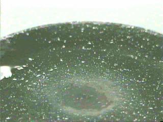
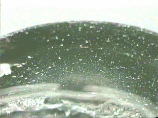
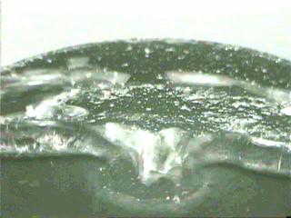
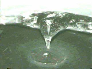
224 Chapter 6 Drop Mobility Figure 6.5 Steam condensing onto a copper superhydrophobic circular gradient surface. Figure 6.6 Evaporation of water from a copper superhydrophobic circular gradient surface.