Definition of Statistics Statistics Branches of Statistics Descriptive statistics Inferential statistics

Transcription

1 What is Statistics? Definition of Statistics Statistics is the science of collecting, organizing, analyzing, and interpreting data in order to make a decision. Branches of Statistics The study of statistics has two major branches descriptive(eploratory) statistics and inferential statistics. Descriptive statistics is the branch of statistics that involves the organization, summarization, and display of data. Inferential statistics is the branch of statistics that involves using a sample to draw conclusions about population. A basic tool in the study of inferential statistics is probability.

2 Scatterplots and Correlation

3 Displaying relationships: Scatterplots Interpreting scatterplots Adding categorical variables to scatterplots Measuring linear association: correlation r Facts about correlation

4 Response variable measures an outcome of a study. An eplanatory variable eplains, influences or cause changes in a response variable. Independent variable and dependent variable. WARNING: The relationship between two variables can be strongly influenced by other variables that are lurking in the background. Note: There is not necessary to have a cause-and-effect relationship between eplanatory and response variables. Eample. Sales of personal computers and athletic shoes

5 Eample - 1

6 Definitions Sample space: the set of all possible outcomes. We denote S Event: an outcome or a set of outcomes of a random phenomenon. An event is a subset of the sample space. Probability is the proportion of success of an event. Probability model: a mathematical description of a random phenomenon consisting of two parts: S and a way of assigning probabilities to events.

7 Probability distributions Probability distribution of a random variable X: it tells what values X can take and how to assign probabilities to those values. Probability of discrete random variable: list of the possible value of X and their probabilities Probability of continuous random variable: density curve.

8 Measuring linear association: correlation r (The Pearson Product-Moment Correlation Coefficient or Correlation Coefficient) The correlation r measures the strength and direction of the linear association between two quantitative variables, usually labeled X and Y. r = 1 n 1 ( i s )( y i s y y )

9 Facts about correlation What kind of variables do we use? 1. No distinction between eplanatory and response variables.. Both variables should be quantitative Numerical properties 1. 1 r 1. r>0: positive association between variables 3. r<0: negative association between variables 4. If r =1or r = - 1, it indicates perfect linear relationship 5. As r is getting close to 1, much stronger relationship negative relationship positive relationship stronger stronger 6. Effected by a few outliers not resistant. 7. It doesn t describe curved relationships 8. Not easy to guess the value of r from the appearance of a scatter plot

10

11 Some necessary elements of Probability theory and Statistics

12 The NORMAL DISTRIBUTION The normal (or Gaussian) distribution, is a very commonly used (occurring) function in the fields of probability theory, and has wide applications in the fields of: - Pattern Recognition; - Machine Learning; - Artificial Neural Networks and Soft computing; - Digital Signal (image, sound, video etc.) processing - Vibrations, Graphics etc.

13 Its also called a BELL function/curve. The formula for the normal distribution is: p( ) = σ 1 π ep[ 1 ( σ μ ) ] The parameter μ is called the mean or epectation (or median or mode) of the distribution. The parameter σ is the standard deviation; and variance is thus σ.

14 P() p( ) = 1 ep[ σ π 1 ( μ ) σ ] X (013)

15 The % Rule: All normal density curves satisfy the following property which is often referred to as the Empirical Rule: - 68% of the observations fall within 1 standard deviation of the mean, that is, between ( μ σ) and ( μ + σ) - 95% of the observations fall within standard deviations of the mean, that is, between ( μ σ ) and ( μ + σ ) % of the observations fall within 3 standard deviations of the mean, that is, between ( μ 3σ ) and ( μ + 3σ )

16 p( ) = 1 ep[ σ π 1 ( μ ) σ ]

17 The normal distribution p(), with any mean μ and any positive deviation σ, has the following properties: It is symmetric around the mean (μ) of the distribution. It is unimodal: its first derivative is positive for < μ, negative for > μ, and zero only at = μ. It has two inflection points (where the second derivative of f is zero and changes sign), located one standard deviation away from the mean, = μ σ and = μ + σ. It is log-concave. It is infinitely differentiable, indeed supersmooth of order.

18 Also, the standard normal distribution p (with μ = 0 and σ = 1) also has the following properties: Its first derivative p () is:.p(). Its second derivative p () is: ( 1).p() More generally, its n-th derivative : p (n) () is: (-1) n H n ()p(), where, H n is the Hermite polynomial of order n.

19

20 Mathematically, p ( Y ) = 1 ( Y μy ) / σ Y πσ Y ε

21 A normal distribution: 1. is symmetrical (both halves are identical);. is asymptotic (its tails never touch the underlying -ais; the curve reaches to and + and thus must be truncated); 3. has fied and known areas under the curve (these fied areas are marked off by units along the -ais called z-scores; imposing truncation, the normal curve ends at z on the right and z on the left).

22

23

24 Normal Density: ] ) ( 1 ep[ 1 ) ( σ μ π σ = p Bivariate Normal Density: ) (1 ), ( ] ) ( ) )( ( ) [( ) (1 1 y y y y y y y y y y e y p ρ σ πσ σ μ σ σ μ μ ρ σ μ ρ = + - Correlation Coefficient S.D.; - Mean; - y ρ σ μ Visualize ρ as equivalent to the orientation of the -D Gabor filter. For as a discrete random variable, the epected value of : = = = n i i i P E 1 ) ( ) ( μ E() is also called the first moment of the distribution. The k th moment is defined as: = = n i i k i k P E 1 ) ( ) ( P( i ) is the probability of = i.

25 Second, third, moments of the distribution p() are the epected values of:, 3, The k th central moment is defined as: = = n i i k k P E 1 ) ( ) ( ] ) [( μ μ Thus, the second central moment (also called Variance) of a random variable is defined as: ] ) [( ] )} ( [{ E E E μ σ = = S.D. of is σ. If z is a new variable: z= a + by; Then E(z) = E(a + by)=ae() + be(y). ) ( ) ( ] ) [( ] )} ( [{ E E E E E μ μ μ μ σ = + = = = ) ( μ = σ + E Thus

26 σ = E μ )( y μ )] Covariance of and y, is defined as: y [( y Covariance indicates how much and y vary together. The value depends on how much each variable tends to deviate from its mean, and also depends on the degree of association between and y. Correlation between and y: ρ y = σ σ y σ y μ = E[( )( σ y μ σ y y )] Property of correlation coefficient: 1 ρ 1 y For Z = a + by ; E[( z μ z ) ] = a σ + ab σ y + b σ y ; If σ y = 0, σ z = a σ + b σ y

27 ρ y = σ σ y σ y = μ E[( )( σ y μ σ y y )] The correlation coefficient can also be viewed as the cosine of the angle between the two vectors (R D ) of samples drawn from the two random variables. This method only works with centered data, i.e., data which have been shifted by the sample mean so as to have an average of zero.

28 Other PDFs: P( ) = λ! e λ; Poisson λ > 0 Binomial Cauchy

29 LAPLACE: Read about: Double Eponential Density: 1 a b P( ) = e ; b Central Limit Theorem Uniform Distribution Geometric Distribution Quantile-Quantile (QQ) Plot Probability-Probability (P-P) Plot

30 Sample mean is defined as: = = = = n i i n i i i n P 1 1 ~ 1 ) ( where, P( i ) = 1/n. Sample Variance is: = = n i i n 1 ~ ) ( 1 σ Higher order moments may also be computed: 4 ~ 3 ~ ) ( ; ) ( E E i i Covariance of a bivariate distribution: = = = n i y y y y n y E 1 ~ ~ ) )( ( 1 )] )( [( μ μ σ PROB. & STAT. Contd.

31 MAXIMUM LIKELIHOOD ESTIMATE (MLE) The ML estimate (MLE) of a parameter is that value which, when substituted into the probability distribution (or density), produces that distribution for which the probability of obtaining the entire observed set of samples is maimized. Problem: Find the maimum likelihood estimate for μ in a normal distribution. Normal Density: ] ) ( 1 ep[ 1 ) ( σ μ π σ = p Assuming all random samples to be independent: = = Π = = ) ( ) ( )... ( ),,,, ( i n i n n p p p p ] ) ( 1 ep[ ) ( 1 1 / = n i n n σ μ σ π σ Taking derivative (w.r.t. μ ) of the LOG of the above: = = = n i i n i i n 1 1 ] [ 1 ). ( 1 μ σ μ σ Setting this term = 0, we get: ~ 1 1 n n i i = = = μ Also read about MAP estimate Baye s is an eample.

32

33 Sampling Distributions

34 What are the main types of sampling and how is each done? Simple Random Sampling: A simple random sample (SRS) of size n is produced by a scheme which ensures that each subgroup of the population of size n has an equal probability of being chosen as the sample. Stratified Random Sampling: Divide the population into "strata". There can be any number of these. Then choose a simple random sample from each stratum. Combine those into the overall sample. That is a stratified random sample. (Eample: Church A has 600 women and 400 women as members. One way to get a stratified random sample of size 30 is to take a SRS of 18 women from the 600 women and another SRS of 1 men from the 400 men.) Multi-Stage Sampling: Sometimes the population is too large and scattered for it to be practical to make a list of the entire population from which to draw a SRS. For instance, when the a polling organization samples US voters, they do not do a SRS. Since voter lists are compiled by counties, they might first do a sample of the counties and then sample within the selected counties. This illustrates two stages. <* SRC: WIKI *>

35 In statistics, a simple random sample is a subset of individuals (a sample) chosen from a larger set (a population). Each individual is chosen randomly and entirely by chance, such that each individual has the same probability of being chosen at any stage during the sampling process, and each subset of k individuals has the same probability of being chosen for the sample as any other subset of k individuals. This process and technique is known as simple random sampling, and should not be confused with systematic random sampling. A simple random sample is an unbiased surveying technique. Systematic sampling (Sys-S) is a statistical method involving the selection of elements from an ordered sampling frame. The most common form of systematic sampling is an equi-probability method. In this approach, progression through the list is treated circularly, with a return to the top once the end of the list is passed. The sampling starts by selecting an element from the list at random and then every k-th element in the frame is selected, where k, the sampling interval (sometimes known as the skip): this is calculated as: k = N/n where n is the sample size, and N is the population size.

36 Systematic sampling (Sys-S) Eample: Suppose a supermarket wants to study buying habits of their customers, then using systematic sampling they can choose every 10th or 15th customer entering the supermarket and conduct the study on this sample. This is random sampling with a system. From the sampling frame, a starting point is chosen at random, and choices thereafter are at regular intervals. For eample, suppose you want to sample 8 houses from a street of 10 houses. 10/8=15, so every 15th house is chosen after a random starting point between 1 and 15. If the random starting point is 11, then the houses selected are 11, 6, 41, 56, 71, 86, 101, and 116.

37 Sampling With Replacement and Sampling Without Replacement Consider a population of potato sacks, each of which has either 1, 13, 14, 15, 16, 17, or 18 potatoes, and all the values are equally likely. Suppose that, in this population, there is eactly one sack with each number. So the whole population has seven sacks. Sampling with replacement: If I sample two with replacement, then I first pick one (say 14). I had a 1/7 probability of choosing that one. Then I replace it. Then I pick another. Every one of them still has 1/7 probability of being chosen. And there are eactly 49 different possibilities here. Sampling without replacement: If I sample two without replacement, then I first pick one (say 14). I had a 1/7 probability of choosing that one. Then I pick another. At this point, there are only si possibilities: 1, 13, 15, 16, 17, and 18. So there are only 4 different possibilities here (again assuming that we distinguish between the first and the second.)

38 Sampling distribution The sampling distribution of a statistic (not parameter) is the distribution of values taken by the statistic (not parameter) in all possible samples of the same size from the same population.

39 Sampling Distribution Introduction In real life calculating parameters of populations is prohibitive because populations are very large. Rather than investigating the whole population, we take a sample, calculate a statistic related to the parameter of interest, and make an inference. The sampling distribution of the statistic is the tool that tells us how close is the statistic to the parameter.

40 Sample Statistics as Estimators of Population Parameters A sample statistic is a numerical measure of a summary characteristic of a sample. A population parameter is a numerical measure of a summary characteristic of a population. An estimator of a population parameter is a sample statistic used to estimate or predict the population parameter. An estimate of a parameter is a particular numerical value of a sample statistic obtained through sampling. A point estimate is a single value used as an estimate of a population parameter.

41 Estimators The sample mean, X, is the most common estimator of the population mean, μ. The sample variance, s, is the most common estimator of the population variance, σ. The sample standard deviation, s, is the most common estimator of the population standard deviation, σ. The sample proportion, pˆ, is the most common estimator of the population proportion, p.

42 Sampling Distribution of X The sampling distribution of X is the probability distribution of all possible values the random variable X may assume when a sample of size n is taken from a specified population.

43 Sampling Distribution of the Mean An eample A die is thrown infinitely many times. Let X represent the number of spots showing on any throw. The probability distribution of X is p() 1/6 1/6 1/6 1/6 1/6 1/6 E(X) = 1(1/6) + (1/6) + 3(1/6)+.= 3.5 V(X) = (1-3.5) (1/6) + (-3.5) (1/6) +. =.9

44 Throwing a dice twice sampling distribution of sample mean Suppose we want to estimate μ from the mean of a sample of size n =. What is the distribution of?

45 Throwing a die twice sample mean Sample Mean Sample Mean Sample Mean 1 1, ,1 5 5,1 3 1, ,.5 6 5, ,3 15 3, , , , , , , , , , , , , , , 0 4, 3 3 6, 4 9, , , ,4 3 4, ,4 5 11, , , , , ,6 6

46 6/36 5/36 4/36 3/36 /36 1/36 Sample Mean Sample Mean Sample Mean 1 1, ,1 5 5,1 3 The 1, distribution ,of.5 when 6 5,n = ,3 15 3, , , , , , , ,5 σ 5 6 Note 1,6 : 3.5 μ = 18 μ 3,6 and σ = 5, , , , , 0 4, 3 3 6, 4 9, , , ,4 3 4, ,4 5 11, , , , , , E( ) =1.0(1/36)+ 1.5(/36)+.=3.5 V(X) = ( ) (1/36)+ ( ) (/36)... = 1.46

47 Sampling Distribution of the Mean n = 5 μ σ = 3.5 =.5833 ( = σ 5 ) 6 n = 10 μ σ = 3.5 =.917 ( = σ ) 10 n = 5 μ σ = 3.5 =.1167 ( = σ ) 5

48 Sampling Distribution of the Mean n = 5 μ σ = 3.5 =.5833 ( = σ 5 ) n = 10 μ σ = 3.5 =.917 ( = σ ) 10 n = 5 μ σ = 3.5 =.1167 ( = σ ) 5 Notice that σ is smaller than. σ. The larger the sample size the smaller σ. Therefore, tends to fall closer to μ, as the sample size increases.

49 Relationships between Population Parameters and the Sampling Distribution of the Sample Mean The epected value of the sample mean is equal to the population mean: E( X) = μ = μ X X The variance of the sample mean is equal to the population variance divided by the sample size: V ( X ) = σ = The standard deviation of the sample mean, known as the standard error of the mean, is equal to the population standard deviation divided by the square root of the sample size: X σ n σ X s.e. = SD( X) =σ = X n X

50 Law of Large Number

51 How sample means approach the population mean (μ=5).

52 Eample - what would happen in many samples?

53 Recall Some Features of the Sampling Distribution It will approimate a normal curve even if the population you started with does NOT look normal Sampling distribution serves as a bridge between the sample and the population

54 Mean of a sample mean

55 Standard Deviation of a sample mean

56 Third Property: Sample Size and the Standard Deviation The larger the sample size, the smaller the standard deviation of the mean Or As n increases, the standard deviation of the mean decreases

57

58 Sampling distribution of a sample mean Definition: For a random variable and a given sample size n, the distribution of the variable, that is the distribution of all possible sample means, is called the sampling distribution of the sample mean.

59 Sampling distribution of the sample mean σ / n Case 1. Population follows Normal distribution Draw an SRS of size n from any population. Repeat sampling. Population follows a Normal distribution with mean µ and standard deviation σ. Sampling distribution of follows normal distribution as follows: N(µ, σ/ n ).

60 Eample (The population distribution follow a Normal distribution, then so does the sample mean)

61 The central limit theorem This theorem tells us: 1. Small samples: Shape of sampling distribution is less normal. Large sample: Shape of sampling distribution is more normal.

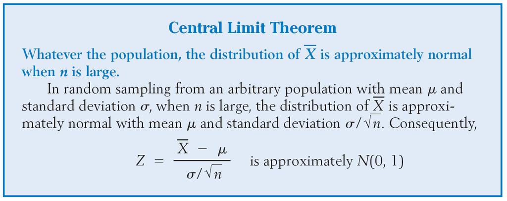
62 Sampling distribution of the sample mean Case. Population follows any distribution (CLT: Central limit theorem) Draw an SRS of size n from any population. Repeat sampling. Population follows a distribution with mean µ and standard deviation σ. When n is large (n>=30), sampling dist of follows approimately Normal distribution as follows N(µ, σ/ n ).

63 The Central Limit Theorem When sampling from a population with mean μ and finite standard deviation σ, the sampling distribution of the sample mean will tend to be a normal distribution with σ mean μ and standard deviation as n the sample size becomes large (n >30). P(X) P(X) n = 5 n = 0 Large n X X For large enough n: X ~ N( μ, σ / n) f(x) μ X

64 The Central Limit Theorem Applies to Sampling Distributions from Any Population Normal Uniform Skewed General Population n = n = 30 μ X μ X μ X μ X

65 Student s t Distribution If the population standard deviation, σ, is unknown, replace σ with the sample standard deviation, s. If the population is normal, the resulting statistic: X μ t = s / has a t distribution with (n - 1) degrees of freedom. n The t is a family of bell-shaped and symmetric distributions, one for each number of degree of freedom. The epected value of t is 0. The variance of t is greater than 1, but approaches 1 as the number of degrees of freedom increases. The t distribution approaches a standard normal as the number of degrees of freedom increases. When the sample size is small (<30) we use t distribution. 0 μ Standard normal t, df=0 t, df=10

66 Sampling Distributions Finite Population Correction Factor If the sample size is more than 5% of the population size and the sampling is done without replacement, then a correction needs to be made to the standard error of the means. σ = σ n N N n 1

67 Sampling Distribution of Standard Deviation of Finite Population Infinite Population σ = σ ( ) n N N n 1 σ = σ n A finite population is treated as being infinite if n/n <.05. ( N n )/( N 1 ) is the finite correction factor. σ is referred to as the standard error of the mean.

68 The Sampling Distribution of the Sample Proportion, p The sample proportion is the percentage of successes in n binomial trials. It is the number of successes, X, divided by the number of trials, n. P(X) n=, p = 0.3 X Sample proportion: p = X n P(X) n=10,p=0.3 As the sample size, n, increases, the sampling distribution of p approaches a normal distribution with mean p and standard deviation p( 1 p) n P(X) n=15, p = X X ^p

69

70 Statistical inference: CLT, confidence intervals, p-values

71 The process of making guesses about the truth Truth (not observable) μ N i= = 1 N from a sample. Population parameters σ = N i= 1 ( μ) i N Sample (observation) Sample statistics ˆμ ˆ σ = s i= 1 n 1 Make guesses about the whole population X = n n i= 1 = n = n ( X i *hat notation ^ is often used to indicate estitmate n )

72 Statistics vs. Parameters Sample Statistic any summary measure calculated from data; e.g., could be a mean, a difference in means or proportions, an odds ratio, or a correlation coefficient E.g., the mean Vit-D level in a sample of 100 men is 63 nmol/l E.g., the correlation coefficient between vit-d and cognitive function in the sample of 100 men is 0.15 Population parameter the true value/true effect in the entire population of interest E.g., the true mean vitamin D in all middle-aged and older European men is 6 nmol/l E.g., the true correlation between vitamin D and cognitive function in all middle-aged and older European men is 0.15

73 Eample 1: cognitive function and vitamin D Hypothetical data loosely based on [1]; cross-sectional study of 100 middle-aged and older European men. Estimation: What is the average serum vitamin D in middle-aged and older European men? Sample statistic: mean vitamin D levels Hypothesis testing: Are vitamin D levels and cognitive function correlated? Sample statistic: correlation coefficient between vitamin D and cognitive function, measured by the Digit Symbol Substitution Test (DSST). 1. Lee DM, Tajar A, Ulubaev A, et al. Association between 5-hydroyvitamin D levels and cognitive performance in middle-aged and older European men. J Neurol Neurosurg Psychiatry. 009 Jul;80(7):7-9.

74 Distribution of a trait: vitamin D Right-skewed! Mean= 63 nmol/l Standard deviation = 33 nmol/l

75 Distribution of a trait: DSST Normally distributed Mean = 8 points Standard deviation = 10 points

76 Distribution of a statistic Statistics follow distributions too But the distribution of a statistic is a theoretical construct. Statisticians ask a thought eperiment: how much would the value of the statistic fluctuate if one could repeat a particular study over and over again with different samples of the same size? By answering this question, statisticians are able to pinpoint eactly how much uncertainty is associated with a given statistic.

77 Distribution of a statistic Two approaches to determine the distribution of a statistic: 1. Computer simulation Repeat the eperiment over and over again virtually! More intuitive; can directly observe the behavior of statistics.. Mathematical theory Proofs and formulas! More practical; use formulas to solve problems.

78 Coin tosses Conclusions: We usually get between 40 and 60 heads when we flip a coin 100 times. It s etremely unlikely that we will get 30 heads or 70 heads (didn t happen in 30,000 eperiments!).

79 Distribution of the sample mean, computer simulation 1. Specify the underlying distribution of vitamin D in all European men aged 40 to 79. Right-skewed Standard deviation = 33 nmol/l True mean = 6 nmol/l (this is arbitrary; does not affect the distribution). Select a random sample of 100 virtual men from the population. 3. Calculate the mean vitamin D for the sample. 4. Repeat steps () and (3) a large number of times (say 1000 times). 5. Eplore the distribution of the 1000 means.

80 Distribution of mean vitamin D (a sample statistic) Normally distributed! Surprise! Mean= 6 nmol/l (the true mean) Standard deviation = 3.3 nmol/l

81 Distribution of mean vitamin D (a sample statistic) Normally distributed (even though the trait is right-skewed!) Mean = true mean Standard deviation = 3.3 nmol/l The standard deviation of a statistic is called a standard error s The standard error of a mean = n

82 If I increase the sample size to n=400 Standard error = 1.7 nmol/l s 33 = = 1.7 n 400

83 If I increase the variability of vitamin D (the trait) to SD=40 Standard error = 4.0 nmol/l s n = 40 =

84 Mathematical Theory The Central Limit Theorem! If all possible random samples, each of size n, are taken from any population with a mean μ and a standard deviation σ, the sampling distribution of the sample means (averages) will: 1. have mean: μ = μ. have standard deviation: σ = σ n 3. be approimately normally distributed regardless of the shape of the parent population (normality improves with larger n). It all comes back to Z!

85 Symbol Check μ σ The mean of the sample means. The standard deviation of the sample means. Also called the standard error of the mean.

86 Mathematical Proof (optional!) If X is a random variable from any distribution with known mean, E(), and variance, Var(), then the epected value and variance of the average of n observations of X is: ) ( ) ( ) ( ) ( ) ( 1 1 E n ne n E n E X E n i n i i n = = = = = = n Var n nvar n Var n Var X Var n i n i i n ) ( ) ( ) ( ) ( ) ( 1 1 = = = = = =

87 Computer simulation of the CLT: 1. Pick any probability distribution and specify a mean and standard deviation.. Tell the computer to randomly generate 1000 observations from that probability distributions E.g., the computer is more likely to spit out values with high probabilities 3. Plot the observed values in a histogram. 4. Net, tell the computer to randomly generate 1000 averages-of- (randomly pick and take their average) from that probability distribution. Plot observed averages in histograms. 5. Repeat for averages-of-10, and averages-of-100.

88 Uniform on [0,1]: average of 1 (original distribution)

89 Uniform: 1000 averages of

90 Uniform: 1000 averages of 5

91 Uniform: 1000 averages of 100

92 ~Ep(1): average of 1 (original distribution)

93 ~Ep(1): 1000 averages of

94 ~Ep(1): 1000 averages of 5

95 ~Ep(1): 1000 averages of 100

96 ~Bin(40,.05): average of 1 (original distribution)

97 ~Bin(40,.05): 1000 averages of

98 ~Bin(40,.05): 1000 averages of 5

99 ~Bin(40,.05): 1000 averages of 100

100 The Central Limit Theorem: (revisited) If all possible random samples, each of size n, are taken from any population with a mean μ and a standard deviation σ, the sampling distribution of the sample means (averages) will: 1. have mean: μ = μ. have standard deviation: σ = σ n 3. be approimately normally distributed regardless of the shape of the parent population (normality improves with larger n)

101

102 Distribution of the sample mean Statistical inference about the population mean is of prime practical importance. Inferences about this parameter are based on the sample mean and its sampling distribution.

103

104 Consider a population with mean 8 and standard deviation 1. If a random sample of size 64 is selected, what is the probability that the sample mean will lie between 80.8 and 83.? Solution: We have μ = 8 and σ = 1. Since n = 64 is large, the central limit theorem tells us that the distribution of the sample mean is approimately normal with σ 1 E( X ) = μ = 8, sd( X ) = = = 1.5 n 64 Converting to the standard normal variable: Z Thus, P[80.8 < X μ = = σ n X = P[.8 < Z Eample on probability calculations for the sample mean X < 83.] = P[(80.8 8) /1.5 < Z < (83. 8) /1.5] <.8] = =.576

105

106

107

108 The Central Limit Theorem more formally

109 The Central Limit Theorem If repeated random samples of size N are drawn from a population that is normally distributed along some variable Y, having a mean μ and a standard deviation σ, then the sampling distribution of all theoretically possible sample means will be a normal distribution having a mean μ and a standard deviation σˆ given by s Y n [Sirkin (1999), p. 39]

110 Mean Standard Deviation Variance Universe μ Y σ Y σ Y Sampling μ Y σˆy σˆ Y Distribution _ Sample Y s Y s Y

111 The Standard Error σˆ = s Y N where s Y = sample standard deviation and N = sample size

112 Let's assume that we have a random sample of 00 USC undergraduates. Note that this is both a large and a random sample, hence the Central Limit Theorem applies to any statistic that we calculate from it. Let's pretend that we asked these 00 randomly-selected USC students to tell us their grade point average (GPA). (Note that our statistical calculations assume that all 00 [a] knew their current GPA and [b] were telling the truth about it.) We calculated the mean GPA for the sample and found it to be.58. Net, we calculated the standard deviation for these self-reported GPA values and found it to be 0.44.

113 The standard error is nothing more than the standard deviation of the sampling distribution. The Central Limit Theorem tells us how to estimate it: σˆ = s Y N

114 The standard error is estimated by dividing the standard deviation of the sample by the square root of the size of the sample. In our eample, σˆ = ˆ σ = ˆ = σ

115 An eample illustrating the central limit theorem Distributions of for n = 3 and n = 10 in sampling from an asymmetric population.

116 Recapitulation 1. The Central Limit Theorem holds only for large, random samples.. When the Central Limit Theorem holds, the mean of the sampling distribution μ is equal to the mean in the universe (also μ). 3. When the Central Limit Theorem holds, the standard deviation of the sampling distribution (called the standard error, ) is estimated by σˆ = s Y N σˆy

117 Recapitulation (continued) 4. When the Central Limit Theorem holds, the sampling distribution is normally shaped. 5. All normal distributions are symmetrical, asymptotic, and have areas that are fied and known.

118 In statistics, a confidence interval (CI) is a type of interval estimate of a population parameter. It is an observed interval (i.e., it is calculated from the observations), in principle different from sample to sample, that potentially includes the unobservable true parameter of interest. How frequently the observed interval contains the true parameter if the eperiment is repeated is called the confidence level. In other words, if confidence intervals are constructed in separate eperiments on the same population following the same process, the proportion of such intervals that contain the true value of the parameter will match the given confidence level. <WIKI> Confidence intervals consist of a range of values (interval) that act as good estimates of the unknown population parameter. However, the interval computed from a particular sample does not necessarily include the true value of the parameter. Confidence intervals are commonly reported in tables or graphs, to show the reliability of the estimates. For eample, a confidence interval can be used to describe how reliable survey results are.

119 In applied practice, confidence intervals are typically stated at the 95% confidence level. However, when presented graphically, confidence intervals can be shown at several confidence levels, for eample 90%, 95% and 99%. Certain factors may affect the confidence interval size including size of sample, level of confidence, and population variability. A larger sample size normally will lead to a better estimate of the population parameter. In statistical inference, the concept of a confidence distribution (CD) has often been loosely referred to as a distribution function on the parameter space that can represent confidence intervals of all levels for a parameter of interest. In statistics, a confidence region is a multi-dimensional generalization of a confidence interval. It is a set of points in an n- dimensional space, often represented as an ellipsoid around a point which is an estimated solution to a problem, although other shapes can occur. A confidence band is used in statistical analysis to represent the uncertainty in an estimate of a curve or function based on limited or noisy data.

120 The eplanation of a confidence interval can amount to something like: "The confidence interval represents values for the population parameter for which the difference between the parameter and the observed estimate is not statistically significant at the 10% level (assuming 90% confidence interval as an eample). In fact, this relates to one particular way in which a confidence interval may be constructed. The following applies: If the true value of the parameter lies outside the 90% confidence interval once it has been calculated, then a sampling event has occurred which had a probability of 10% (or less) of happening by chance. A 95% confidence interval does not mean that for a given realised interval calculated from sample data there is a 95% probability the population parameter lies within the interval. Once an eperiment is done and an interval calculated, this interval either covers the parameter value or it does not; it is no longer a matter of probability. The 95% probability relates to the reliability of the estimation procedure, not to a specific calculated interval.

121 A 95% confidence interval does not mean that 95% of the sample data lie within the interval. A confidence interval is not a range of plausible values for the sample parameter, though it may be understood as an estimate of plausible values for the population parameter. A particular confidence interval of 95% calculated from an eperiment does not mean that there is a 95% probability of a sample parameter from a repeat of the eperiment falling within this interval.

122

123

124

125

126

127

128

129

130

131

132

133

134

135 Inference about a Population Mean

136

137

138

139

140

141

142

143

144 Recapitulation 1. Statistical inference involves generalizing from a sample to a (statistical) universe.. Statistical inference is only possible with random samples. 3. Statistical inference estimates the probability that a sample result could be due to chance (in the selection of the sample). 4. Sampling distributions are the keys that connect (known) sample statistics and (unknown) universe parameters. 5. Alpha (significance) levels are used to identify critical values on sampling distributions.

145 The Chi-Square Test 145

146 Significance Test If the distributions of the second variable are nearly the same given the category of the first variable, then we say that there is not an association between the two variables. If there are significant differences in the distributions, then we say that there is an association between the two variables. Significance test is needed to draw a conclusion. 146

147 Hypothesis Test Hypotheses: Null: the percentages for one variable are the same for every level of the other variable (no difference in conditional distributions). (No real relationship). Alt: the percentages for one variable vary over levels of the other variable. (Is a real relationship). 147

148 Null hypothesis: The percentages for one variable are the same for every level of the other variable. (No real relationship). Quality of life Canada United States Much better 4% 5% Somewhat better 3% 3% About the same 31% 36% Somewhat worse 16% 13% Much worse 6% 3% Total 100% 100% For eample, could look at differences in percentages between Canada and U.S. for each level of Quality of life : 4% vs. 5% for those who felt Much better, 3% vs. 3% for Somewhat better, etc. Problem of multiple comparisons! 148

149 Hypothesis Test H 0 : no real relationship between the two categorical variables that make up the rows and columns of a two-way table To test H 0, compare the observed counts in the table (the original data) with the epected counts (the counts we would epect if H 0 were true) if the observed counts are far from the epected counts, that is evidence against H 0 in favor of a real relationship between the two variables 149

150 3. Epected Counts The epected count in any cell of a two-way table (when H 0 is true) is epected count = (row total) (column total) table total For the observed data to the right, find the epected value for each cell: Quality of life Canada United States Total Much better Somewhat better About the same Somewhat worse Much worse Total For the epected count of Canadians who feel Much better (epected count for Row 1, Column 1): (row1 total) (column1 total) epected count = = = table total

151 Observed counts: Compare to see if the data support the null hypothesis Epected counts: Quality of life Canada United States Much better Somewhat better About the same Somewhat worse 50 8 Much worse Quality of life Canada United States Much better Somewhat better About the same Somewhat worse Much worse

152 4. Chi-Square Statistic To determine if the differences between the observed counts and epected counts are statistically significant (to show a real relationship between the two categorical variables), we use the chi-square statistic: X = ( observed count epected count ) epected count where the sum is over all cells in the table. 15

153 Chi-Square Statistic The chi-square statistic is a measure of the distance of the observed counts from the epected counts is always zero or positive is only zero when the observed counts are eactly equal to the epected counts large values of X are evidence against H 0 because these would show that the observed counts are far from what would be epected if H 0 were true 153

154 Observed counts Quality of life Canada United States Much better Somewhat better About the same Somewhat worse 50 8 Much worse X ( ) ( ) = = = Epected counts Canada United States

155 5. Chi-Square Test Calculate value of chi-square statistic Find P-value in order to reject or fail to reject H 0 use chi-square table for chi-square distribution (net few slides) from computer output 155

156 Chi-Square Distributions Family of distributions that take only positive values and are skewed to the right Specific chi-square distribution is specified by giving its degrees of freedom (similar to t dist.) 156

157 Chi-Square Test Chi-square test for a two-way table with r rows and c columns uses critical values from a chi-square distribution with (r 1) (c 1) degrees of freedom P-value is the area to the right of X under the density curve of the chi-square distribution use chi-square table P-value = P(X >= X obs ) 157

158 6. Uses of the Chi-Square Test Tests the null hypothesis H 0 : no relationship between two categorical variables when you have a two-way table from either of these situations: Independent SRSs from each of several populations, with each individual classified according to one categorical variable [Eample: Health Care case study: two samples (Canadians & Americans); each individual classified according to Quality of life ] A single SRS with each individual classified according to both of two categorical variables [Eample: Sample of 835 subjects, with each classified according to their Job Grade (1,, 3, or 4) and their Marital Status (Single, Married, Divorced, or Widowed)] 158

159 Chi-Square Test: Requirements The chi-square test is an approimate method, and becomes more accurate as the counts in the cells of the table get larger The following must be satisfied for the approimation to be accurate: No more than 0% of the epected counts are less than 5 All individual epected counts are 1 or greater In particular, all four epected counts in a table should be 5 or greater If these requirements fail, then two or more groups must be combined to form a new ( smaller ) two-way table 159

160 Summary: steps to do chi-square test 1. Find row total, col total, grand total.. Find epected count for each cell. 3. Find test statistic X : df = (r-1)(c-1) X = ( observed count epected count) epected count 4. Use Table E to find P-value: P-value = P(X >= X obs ) 5. Compare P-value with significance level and draw conclusion. 160