Unit 4 Probability. Dr Mahmoud Alhussami

Transcription

1 Unit 4 Probability Dr Mahmoud Alhussami

2 Probability Probability theory developed from the study of games of chance like dice and cards. A process like flipping a coin, rolling a die or drawing a card from a deck is called a probability experiment. An outcome is a specific result of a single trial of a probability experiment. 2

3 Probability distributions Probability theory is the foundation for statistical inference. A probability distribution is a device for indicating the values that a random variable may have. There are two categories of random variables. These are: discrete random variables, and continuous random variables. 3

4 Discrete Probability Distributions Binomial distribution the random variable can only assume 1 of 2 possible outcomes. There are a fixed number of trials and the results of the trials are independent. i.e. flipping a coin and counting the number of heads in 10 trials. Poisson Distribution random variable can assume a value between 0 and infinity. Counts usually follow a Poisson distribution (i.e. number of ambulances needed in a city in a given night) 21 February

5 Discrete Random Variable A discrete random variable X has a finite number of possible values. The probability distribution of X lists the values and their probabilities. 1. Every probability p i is a number between 0 and The sum of the probabilities must be 1. Value of X x 1 x 2 x 3 x k Probability p 1 p 2 p 3 p k Find the probabilities of any event by adding the probabilities of the particular values that make up the event. 21 February

6 Example The instructor in a large class gives 15% each of A s and D s, 30% each of B s and C s and 10% F s. The student s grade on a 4-point scale is a random variable X (A=4). Grade F=0 D=1 C=2 B=3 A=4 Probability What is the probability that a student selected at random will have a B or better? ANSWER: P (grade of 3 or 4)=P(X=3) + P(X=4) = = February

7 Continuous Probability Distributions When it follows a Binomial or a Poisson distribution the variable is restricted to taking on integer values only. Between two values of a continuous random variable we can always find a third. A histogram is used to represent a discrete probability distribution and a smooth curve called the probability density is used to represent a continuous probability distribution. 21 February

8 Continuous Variable A continuous probability distribution is a probability density function. The area under the smooth curve is equal to 1 and the frequency of occurrence of values between any two points equals the total area under the curve between the two points and the x-axis. 8

9 Normal Distribution Also called belt shaped curve, normal curve, or Gaussian distribution. A normal distribution is one that is unimodal, symmetric, and not too peaked or flat. Given its name by the French mathematician Quetelet who, in the early 19 th century noted that many human attributes, e.g. height, weight, intelligence appeared to be distributed normally.

10 Normal Distribution The normal curve is unimodal and symmetric about its mean ( ). In this distribution the mean, median and mode are all identical. The standard deviation ( ) specifies the amount of dispersion around the mean. The two parameters and completely define a normal curve. 21 February

11 Also called a Probability density function. The probability is interpreted as "area under the curve." The random variable takes on an infinite # of values within a given interval The probability that X = any particular value is 0. Consequently, we talk about intervals. The probability is = to the area under the curve. The area under the whole curve = 1. 11

12 12

13 Properties of a Normal Distribution 1. It is symmetrical about. 2. The mean, median and mode are all equal. 3. The total area under the curve above the x-axis is 1 square unit. Therefore 50% is to the right of and 50% is to the left of. 4. Perpendiculars of: ± contain about 68%; ±2 contain about 95%; ±3 contain about 99.7% of the area under the curve. 13

14 The normal distribution 14

15 The Standard Normal Distribution A normal distribution is determined by and. This creates a family of distributions depending on whatever the values of and are. The standard normal distribution has =0 and =1. 15

16 Standard Z Score The standard z score is obtained by creating a variable z whose value is Given the values of and we can convert a value of x to a value of z and find its probability using the table of normal curve areas. 16

17 Importance of Normal Distribution to Statistics Although most distributions are not exactly normal, most variables tend to have approximately normal distribution. Many inferential statistics assume that the populations are distributed normally. The normal curve is a probability distribution and is used to answer questions about the likelihood of getting various particular outcomes when sampling from a population.

18 Probabilities are obtained by getting the area under the curve inside of a particular interval. The area under the curve = the proportion of times under identical (repeated) conditions that a particular range of values will occur. Characteristics of the Normal distribution: It is symmetric about the mean μ. Mean = median = mode. [ bell-shaped curve] 18

19 Why Do We Like The Normal Distribution So Much? There is nothing special about standard normal scores These can be computed for observations from any sample/population of continuous data values The score measures how far an observation is from its mean in standard units of statistical distance But, if distribution is not normal, we may not be able to use Z-score approach. 21 February

20 Normal Distribution Q A Q A Is every variable normally distributed? Absolutely not Then why do we spend so much time studying the normal distribution? Some variables are normally distributed; a bigger reason is the Central Limit Theorem!!!!!!!!!!!!!!!!!!!!!!!!!!!??????????? 21 February

21 Central Limit Theorem describes the characteristics of the "population of the means" which has been created from the means of an infinite number of random population samples of size (N), all of them drawn from a given "parent population". It predicts that regardless of the distribution of the parent population: The mean of the population of means is always equal to the mean of the parent population from which the population samples were drawn. The standard deviation of the population of means is always equal to the standard deviation of the parent population divided by the square root of the sample size (N). The distribution of means will increasingly approximate a normal distribution as the size N of samples increases.

22 Central Limit Theorem A consequence of Central Limit Theorem is that if we average measurements of a particular quantity, the distribution of our average tends toward a normal one. In addition, if a measured variable is actually a combination of several other uncorrelated variables, all of them "contaminated" with a random error of any distribution, our measurements tend to be contaminated with a random error that is normally distributed as the number of these variables increases. Thus, the Central Limit Theorem explains the ubiquity of the famous bell-shaped "Normal distribution" (or "Gaussian distribution") in the measurements domain.

23 Note that the normal distribution is defined by two parameters, μ and σ. You can draw a normal distribution for any μ and σ combination. There is one normal distribution, Z, that is special. It has a μ = 0 and a σ = 1. This is the Z distribution, also called the standard normal distribution. It is one of trillions of normal distributions we could have selected. 23

24 Standard Normal Variable It is customary to call a standard normal random variable Z. The outcomes of the random variable Z are denoted by z. The table in the coming slide give the area under the curve (probabilities) between the mean and z. The probabilities in the table refer to the likelihood that a randomly selected value Z is equal to or less than a given value of z and greater than 0 (the mean of the standard normal). 21 February

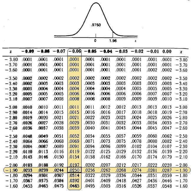
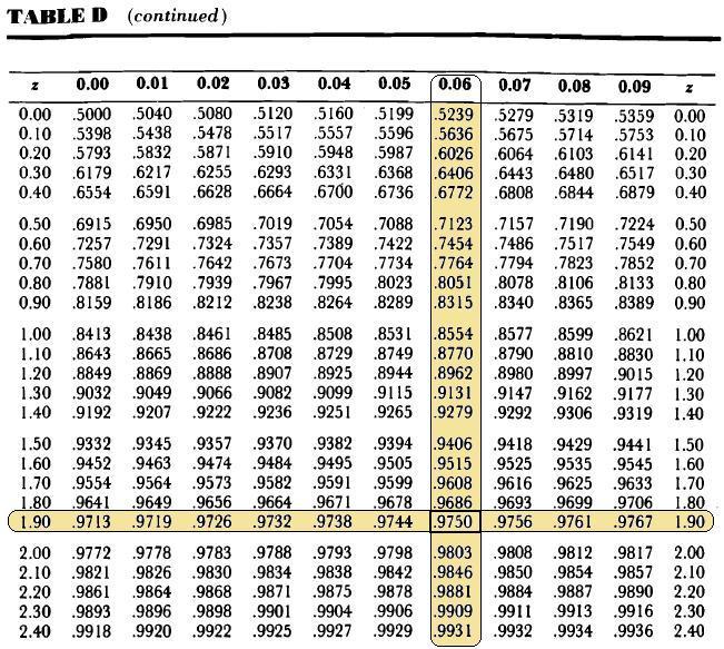
25 Table of Normal Curve Areas 25

26 Standard Normal Curve 21 February

27 Standard Normal Distribution 50% of probability in here probability=0.5 50% of probability in here probability= February

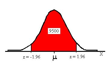
28 Standard Normal Distribution 95% of probability in here 2.5% of probability in here 2.5% of probability in here Standard Normal Distribution with 95% area marked 21 February

29 Calculating Probabilities Probability calculations are always concerned with finding the probability that the variable assumes any value in an interval between two specific points a and b. The probability that a continuous variable assumes the a value between a and b is the area under the graph of the density between a and b. 21 February

30 Finding Probabilities (a) What is the probability that z < ? (1) Sketch a normal curve (2) Draw a line for z = (3) Find the area in the table (4) The answer is the area to the left of the line P(z < -1.96) =

31 31

32 Finding Probabilities 32

33 Finding Probabilities (b) What is the probability that < z < 1.96? (1) Sketch a normal curve (2) Draw lines for lower z = -1.96, and upper z = 1.96 (3) Find the area in the table corresponding to each value (4) The answer is the area between the values. Subtract lower from upper: P(-1.96 < z < 1.96) = =

34 34

35 Finding Probabilities 35

36 Finding Probabilities (c) What is the probability that z > 1.96? (1) Sketch a normal curve (2) Draw a line for z = 1.96 (3) Find the area in the table (4) The answer is the area to the right of the line. It is found by subtracting the table value from : P(z > 1.96) = =

37 Finding Probabilities 37

38 If the weight of males is N.D. with μ=150 and σ=10, what is the probability that a randomly selected male will weigh between 140 lbs and 155 lbs? [Important Note: Always remember that the probability that X is equal to any one particular value is zero, P(X=value) =0, since the normal distribution is continuous.] Normal Distribution 38

39 Solution: X -1 0 Z = ( )/ 10 = s.d. from mean Area under the curve =.3413 (from Z table) Z = ( ) / 10 =+.50 s.d. from mean Area under the curve =.1915 (from Z table) Answer: = Z 39

40 Example For example: What s the probability of getting a math SAT score of 575 or less, =500 and =50? Z i.e., A score of 575 is 1.5 standard deviations above the mean 575 x 500 ( ) Z P( X 575) e dx e dz (50) Yikes! But to look up Z= 1.5 in standard normal chart (or enter into SAS) no problem! =.9332

41 If IQ is ND with a mean of 100 and a S.D. of 10, what percentage of the population will have (a)iqs ranging from 90 to 110? (b)iqs ranging from 80 to 120? Solution: Z = (90 100)/10 = Z = ( )/ 10 = Area between 0 and 1.00 in the Z-table is.3413; Area between 0 and is also.3413 (Z-distribution is symmetric). Answer to part (a) is =

42 (b) IQs ranging from 80 to 120? Solution: Z = (80 100)/10 = Z = ( )/ 10 = Area between =0 and 2.00 in the Z-table is.4772; Area between 0 and is also.4772 (Z-distribution is symmetric). Answer is =

43 Suppose that the average salary of college graduates is N.D. with μ=$40,000 and σ=$10,000. (a) What proportion of college graduates will earn $24,800 or less? (b) What proportion of college graduates will earn $53,500 or more? (c) What proportion of college graduates will earn between $45,000 and $57,000? (d) Calculate the 80th percentile. (e) Calculate the 27th percentile. 43

44 (a) What proportion of college graduates will earn $24,800 or less? Solution: Convert the $24,800 to a Z-score: Z = ($24,800 - $40,000)/$10,000 = Always DRAW a picture of the distribution to help you solve these problems. 44

45 .4357 $24,800 $40, X Z First Find the area between 0 and in the Z-table. From the Z table, that area is Then, the area from to - is = Answer: 6.43% of college graduates will earn less than $24,

46 (b) What proportion of college graduates will earn.4115 $53,500 or more?.0885 Solution: $40,000 $53,500 Convert the $53,500 to a Z-score Z = ($53,500 - $40,000)/$10,000 = Find the area between 0 and in the Z- table:.4115 is the table value. When you DRAW A PICTURE (above) you see that you need the area in the tail: Answer: Thus, 8.85% of college graduates will earn $53,500 or more. Z 46

47 .1915 (c) What proportion of college graduates will earn between $45,000 and $57,000? $40k $45k $57k Z = $45,000 $40,000 / $10,000 =.50 Z = $57,000 $40,000 / $10,000 = Z From the table, we can get the area under the curve between the mean (0) and.5; we can get the area between 0 and 1.7. From the picture we see that neither one is what we need. What do we do here? Subtract the small piece from the big piece to get exactly what we need. Answer: =

48 Parts (d) and (e) of this example ask you to compute percentiles. Every Z-score is associated with a percentile. A Z-score of 0 is the 50 th percentile. This means that if you take any test that is normally distributed (e.g., the SAT exam), and your Z-score on the test is 0, this means you scored at the 50 th percentile. In fact, your score is the mean, median, and mode. 48

49 (d) Calculate the 80 th percentile. Solution: First, what Z-score is associated $40,000 with the 80 th percentile? 0.84 A Z-score of approximately +.84 will give you about.3000 of the area under the curve. Also, the area under the curve between - and 0 is Therefore, a Z-score of +.84 is associated with the 80th percentile. Now to find the salary (X) at the 80 th percentile: Just solve for X: +.84 = (X $40,000)/$10,000 ANSWER X = $40,000 + $8,400 = $48, Z 49

50 (e) Calculate the 27 th percentile. Solution: First, what Z-score is associated.2700 with the 27 th percentile? A Z-score $40,000 of approximately -.61will give you about.2300 of the area under the curve, with.2700 in the tail. (The area under the curve between 0 and -.61 is.2291 which we are rounding to.2300). Also, the area under the curve between 0 and is Therefore, a Z-score of -.61 is associated with the 27 th percentile Now to find the salary (X) at the 27ANSWER th percentile: Just solve for X: =(X $40,000)/$10,000 X = $40,000 - $6,100 = $33,900 Z 50

51